Multiobjective Optimization of Pin-Type Flow Channels Using a Reinterpretation of Murray’s Law

Abstract

Biomimetics has been used to improve performance in several fields of engineering. For flow fields, Murray’s Law has been used to explore branching of channels that carry reactants and products. The applicability of Murray’s Law to flow fields was examined here. The pin-type flow field was used to explore variations and conflicting performance objectives: pressure drop, manufacturability, standard deviation of flow velocity, and channel area. NSGA-II was used to solve a multiobjective optimization problem. Two designs, 3 × 3 and 11 × 11, were analyzed. Results that were similar to previous single-objective studies were obtained, confirming the efficacy of Murray’s Law. Computational fluid dynamics simulations were used to compare optimized and unoptimized designs. The maximum velocity for the 3 × 3 and 11 × 11 cases was lower when Murray’s Law was followed, indicating that it effectively slowed down the flow. Similarly, the flow was much more uniform: the standard deviation of flow velocity in the channels was 94% and 57% lower, respectively, for both cases, compared to the unoptimized designed. Finally, a method to select one optimal solution from a front of non-dominated solutions, the nearest point method, was demonstrated.

1. Introduction

With an increase in the proliferation of clean energy, several promising power generation candidates have been receiving increased attention. Proton-exchange membrane fuel cells (PEMFC), also known as polymer electrolyte membrane fuel cells, are increasing in their adoption as they offer several advantages: being emissions-free, efficient, quiet operation, relatively low-temperature operation, quick start-up, etc. One of the most important components of a fuel cell is the flow distributor or the flow field, accounting for 60–80% of the weight and about 30–50% of the cost [1,2]. These flow fields have been extensively researched over the last few decades and a variety of geometries have emerged has leading candidates, each with its own strengths. 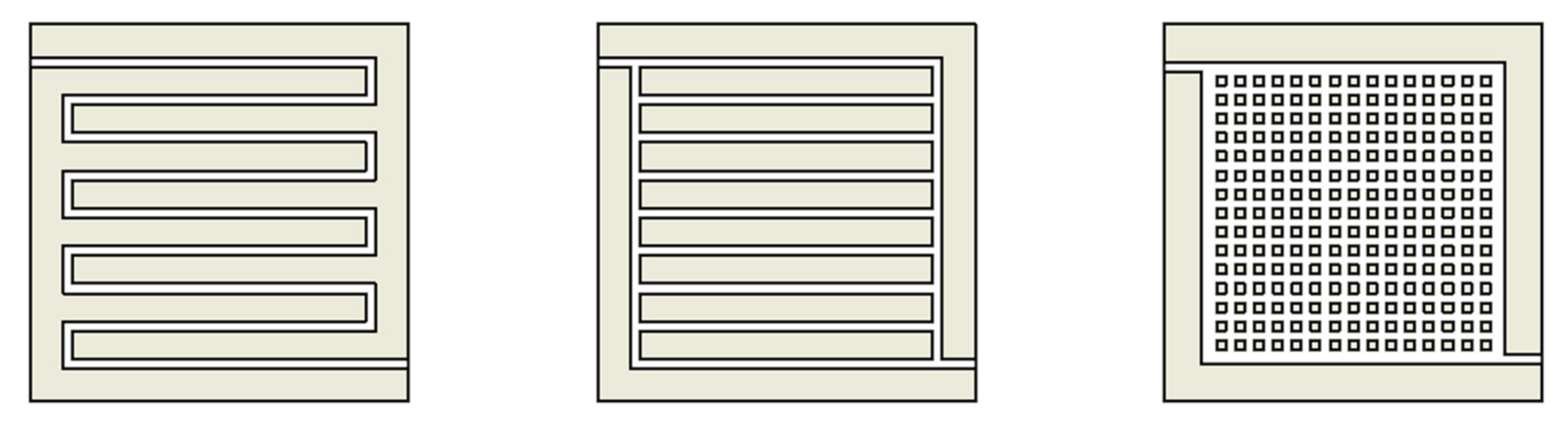Figure 1 shows three such geometries, the serpentine, columnar, and pin-type.

Several design approaches have been used to improve the weaknesses of flow fields to improve overall fuel cell performance. Biomimetic principles have been extensively studied and applied to the design of flow fields. The review paper in [3] summarizes the state of the art in the application of biomimetics to flow field design. Inspiration is derived from bionics, fractals, honeycombs, leaves, lungs, sponges, etc. The study in [4] compared a leaf design and a lung design to common designs. Both designs outperformed conventional designs, but the leaf was found to be the best. The study in [5] explored several nature-inspired designs as well. A significant finding that was common to such designs was that performance improvements attributed to flow fields came from uniform reactant distribution and reduced pressure drop. Wang et al. [6] explored a novel biometric design that demonstrated superior water removal ability when compared to conventional designs.

One explanation that has been proffered to explain the efficacy of leaf-type or lung-type designs is Murray’s Law [7]. This law states that when biological systems pumping fluids in a vessel need to branch, the sum of the cubes of the radii of the daughter vessels should be the cube of the parent vessel to minimize the amount of pumping power necessary for the entire system. This phenomenon has been studied extensively in natural fluid systems carrying air (lungs), blood (blood vessels), sap (leaves), etc. The study reported in [8] is an example of using this law to design flow fields for PEMFCs. Here, the hydraulic diameter was used instead of radius as the channels were rectangular in cross-section. Several design variations based on Murray’s Law can be found in the literature.

The study in [9] is a graduate thesis that specifically explored how Murray’s Law is transposed from biological systems to engineered ones. It pointed out that past studies focused on the geometric and physical aspects of Murray’s Law without taking a closer look at the performance implications. The main finding in a related study by the same author [10] found that about 30% of the overall improvement in performance of a flow field design compared to another could be explained by the increased pressure drop across that flow field. In other words, by forcing the reactants through the flow channels at higher pressures, more of it passed through the gas diffusion layer out of the channel to participate in the electrochemical reaction that produces power. As expected, this increased pressure needs to be constantly maintained and increases the overall operating costs, thereby negating some of the gains.

This study takes a critical look at the basis for the application of Murray’s Law to flow structures in flow fields, specifically the implications of pumping work and metabolic work. There is a dearth of optimization studies pertaining to flow field design, because such geometric optimization tends to be labor-intensive and requires prohibitive computational effort. The few existing studies only look at performance from a flow standpoint, without considering electrical condition or manufacturability. The following section attempts to cast Murray’s Law in a manner more suitable to flow field design and then proposes a multiobjective optimization framework that can implement it efficiently.

2. Examination of Murray’s Law

The primary purpose of the flow field in a fuel cell or similar device is to distribute reactants uniformly to the catalyst layer via the gas diffusion layer and to remove products such as water. Excess reactants are also removed [11]. It must be pointed out that flow fields are not limited to fuel cells. In this study, that is the primary focus: distribution of fluids. Flow fields are integral parts of the design of several other complex engineered structures such as flow batteries, heat exchanges, nuclear reactors, etc. Flow fields are also referred to as flow channels, flow distributors, flow separators, etc.

Typically, there is one inlet into the fuel cell and one outlet. Thus, the flow field must be designed such that the reactants entering from a single point get distributed as uniformly across the entire area of the fuel cell. Any unused reactant that exits is recirculated. Several geometries, such as those in Figure 1, have been studied. The most effective flow fields slow down the inlet gas, allowing sufficient time for diffusion out of the channels and into the gas diffusion layer. The pins in the pin-type design act like obstacles to the flow. This increases diffusion, but also causes a large pressure drop between the inlet and the outlet. The inlet pressure must be high enough to overcome this differential and also to force out any water that would otherwise clog the channels. This is a parasitic loss that designers try to minimize by striking a balance between low pressure drop and performance.

It is thought that by mimicking designs from nature, fuel cells can benefit from the greatest strengths of such designs: uniform reactant distribution and waste product removal while requiring the least pumping effort. For a biological system, minimizing pumping effort is critical to reduce the metabolic burden on the organism. This can be accomplished by evolving large diameter vessels. Further, increasing the number of such vessels will make it easier to reach all parts of the organism to ensure proper distribution of nutrients and removal of waste. However, building and maintaining such large and numerous vessels also exerts a metabolic cost on the organism. Thus, over millions of years, across numerous species, nature has evolved an optimal relationship between the size of vessels, the size of branching vessels, their branching angles, their overall number, etc. [12,13]. In this study, the branching angles and the frequency of branching were not considered. Only the diameter relationship between parent and daughter vessels was considered. Other considerations can be explored in future studies.

Sherman [13] explains the mathematical optimization behind Murray’s Law. It is summarized here in brief. Equation (1) is the Hagen–Poiseuille relationship:

$$p_i=\frac{128\mu L_i{q}_i}{\pi r_i^4}$$

(1)

where p_i is the pressure drop across the ith channel or vessel, μ is the fluid viscosity, L_i is the channel length, q_i is the volumetric flow rate, and r_i is the channel radius (hydraulic diameter, D_i, for rectangular flow field channels). The pumping power, P_f, is:

$$P_f=\frac{a{q}^2}{r^4}$$

(2)

where a = 128 μL/π and L can be taken to be 1 or some arbitrary value. The metabolic power required to maintain a vessel is:

$$P_m=m\pi r^{2}L=b{r}^2$$

(3)

where m is a metabolic coefficient and b = mπL. The total power required is:

$$P=\frac{a{q}^2}{r^4}+b{r}^2$$

(4)

Differentiating with respect to r to find the minimum and rearranging terms produces:

$$q=k{r}^3$$

(5)

where k is a constant. In general, for successive branching generations:

$$\sum q=k\sum r^3$$

(6)

Equation (6) can be written for hydraulic diameters and by eliminating flow by assuming mass continuity.

$$D\left(i\right)=\sum D^3\left(i+1\right)$$

(7)

where D(i) is the hydraulic diameter of the parent branch and D(i + 1) is the hydraulic diameter of the daughter branch. Thus, by balancing the need for larger vessels to reduce pumping work with the need for smaller vessels to reduce metabolic work, the cubic relation is reached.

2.1. Challenges to the Cubic Relation

Studies to validate the cubic relation have pointed out how, for a number of reasons related to the complexity of natural biological systems and preparation of samples, this relation is not perfectly encapsulated in all organisms. Both [13,14] cited studies that found that the expected cubic relation can vary from 2.33 to 3.006. This depends on the generation, i.e., how far down the branching network the measurements are made, the organ, the organism, etc. Sciubba [15] conducted an entropy analysis to point out weaknesses in Murray’s Law applied to biological systems. In Murray’s Law, a symmetric split in the first generation leads to a radius ratio of 1:2^1/3 or 1:0.7937. Sciubba [15] pointed out alternative optimal ratios ranging from 1:0.198 (turbulent flow) to 1:0.8. Equation (4) can be modified to obtain something other than a cubic relation. Either the pumping work or the metabolic work terms can be modified. Assuming the pumping work is accurately described by the Hagen–Poiseuille equation, the metabolic work term’s exponent can be modified:

$$P=\frac{a{q}^2}{r^4}+b{r}^n$$

(8)

where n is taken to be between 1.5 and 3 as an example. Then, the exponent in Equation (7) would be (n + 4)/2. If n = 1.5, then the exponent is 2.75. For 3, it becomes 3.5. Physically, this means that the metabolic cost is not necessarily proportionate to the volume of the vessel as implied in Equation (3).

2.2. Challenges to Applicability to Non-Biological Flow Fields

Both [8,9] caution the designer on improperly applying Murray’s Law, or any biomimetic design, to non-biological flow fields. They point out the high degree of interconnectedness in biological systems, which provides redundancy in the case of damage to a particular vessel. This is usually absent from non-biological flow fields. Biological flow fields also typically transport different types of fluids and their flow rates can vary due to diffusion in and out of the vessels. The directions are also often reversed, with nutrients in one direction and waste in the opposite direction. They postulate that the key strengths of biological designs are to distribute nutrients and remove wastes efficiently, meaning uniformly and with minimum pressure losses. It is further suggested in this study that the entire system’s design and performance must be considered, not just the flow aspect. This is because biological evolution, from which biomimetics draws inspiration, happens on whole organisms and not just individual aspects of organisms.

2.3. Analogy to Metabolic Work

The balance in Murray’s Law and biological systems that emulate it to any extent is between pumping effort and metabolic effort. However, in non-biological flow fields, there is no cost to maintain the structures once the part has been manufactured. Rather, it is argued here that the cost comes from the manufacturability of the design: how much does it cost to design, test, and manufacture a complex branching network as opposed to any simple design like the ones in Figure 1. Thus, the efficacy of Murray’s Law becomes limited if applied improperly. This study considers different metrics that should be considered besides minimization of pressure loss. As mentioned above, a design that is overly complicated will exact a steep manufacturing cost. In the current era dominated by prototypes, a large number of flow fields are still manufactured using rapid prototyping techniques as opposed to mass production techniques. Thus, complex designs portend complex design changes and it becomes prohibitively expensive to make even small changes, analyze them, build, test, and operate them. In this study, manufacturability is proposed as an objective to be minimized. Its exact function would depend on a variety of factors, but, for demonstration purposes, its form is taken to be the same as the metabolic cost, brⁿ. Note that when n = 2, brⁿ = m·V, where V is the volume. The argument here is that the more volume of material that has to be removed in a machining process, the more expensive the manufacturing would be. To account for additional expense due to design, the exponent can be increased to 2.5 or 3. Along with this, it is argued that having a large number of disparate channel widths makes the design and manufacturing process more complex, so minimizing the standard deviation of the channel widths would be desirable. More studies on the manufacturability of flow fields are certainly required. Some comments are provided later in this paper on variations of this function.

Another consideration is conduction. In Reference [16], a pin-type flow field’s channel widths were optimized to make the flow as uniform as possible. The standard deviation of the flow velocity in every channel was minimized. The authors recognized that channels closer to the inlet and outlet would be larger than channels in the middle. However, they also identified that simply making channels large reduces the total amount of “land” or “rib” area, the material around the channels that makes direct contact with the electrolyte and is responsible for current collection. If this area is too small, ohmic losses will overcome any gains in transport losses. They tackled this issue by make the rib area a constraint, at least 40% of total area. In this study, the conduction area is treated as another objective. By minimizing the total channel area, the conduction area is maximized. This also increases the overall strength of the flow field plate. Note that it is a structural component as well and must bear the stress of being bolted to the opposite side flow field plate and holding the fuel cell together.

2.4. Multiobjective Optimization Approach to Flow Field Design

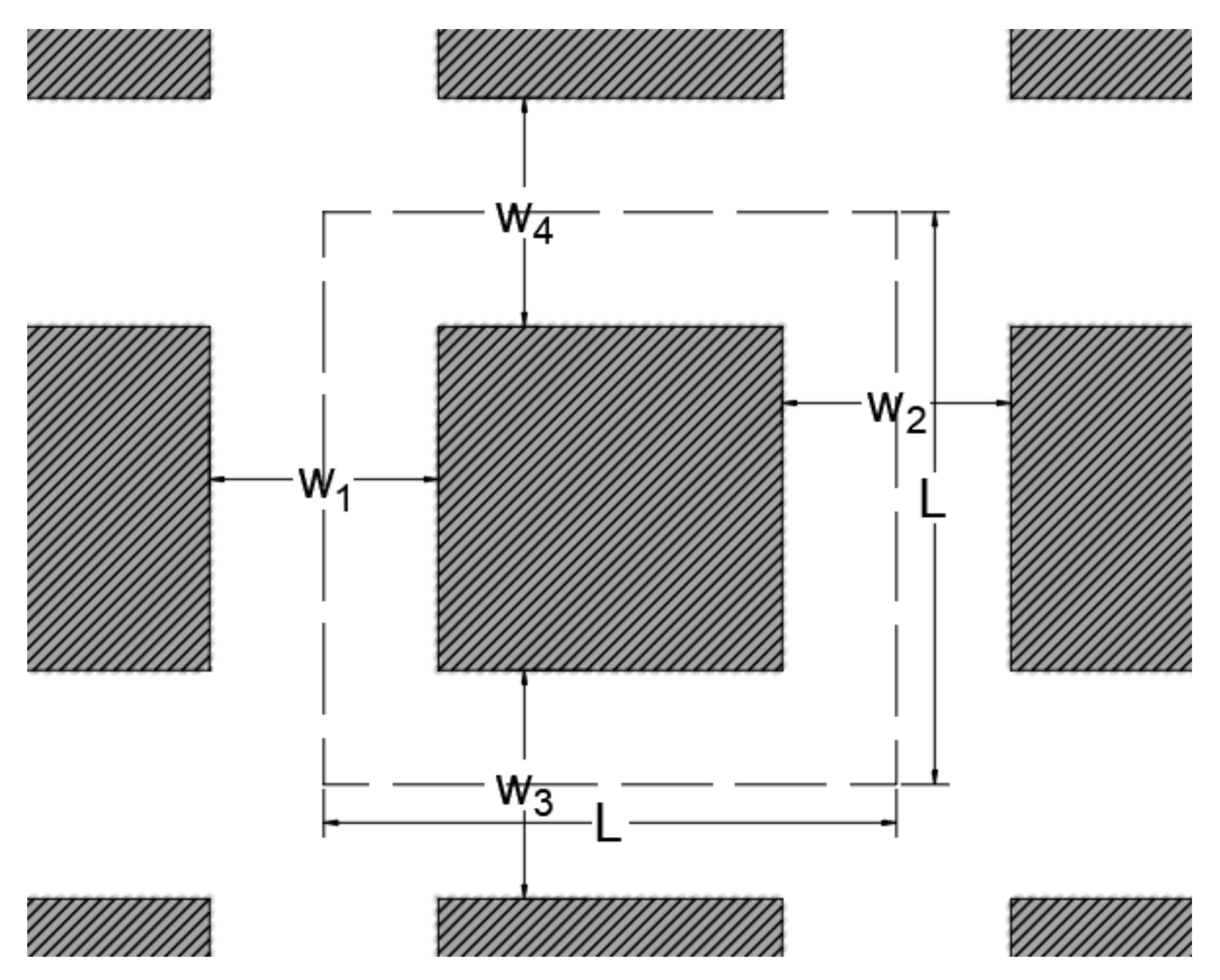
It is clear that existing studies have applied Murray’s Law to design flow fields in a limited sense and without optimization. In this study, flow field optimization is carried out using multiobjective optimization. Rather than programming Murray’s Law, a genetic algorithm, which mimics the principles of natural selection leading to a global optimal solution, was used to find the best channel widths. The objectives of interest were minimization of the pressure drop, the area of the channels (maximizing the area of conduction), the design effort or manufacturability, and the standard deviation of the flow velocities in each channel.

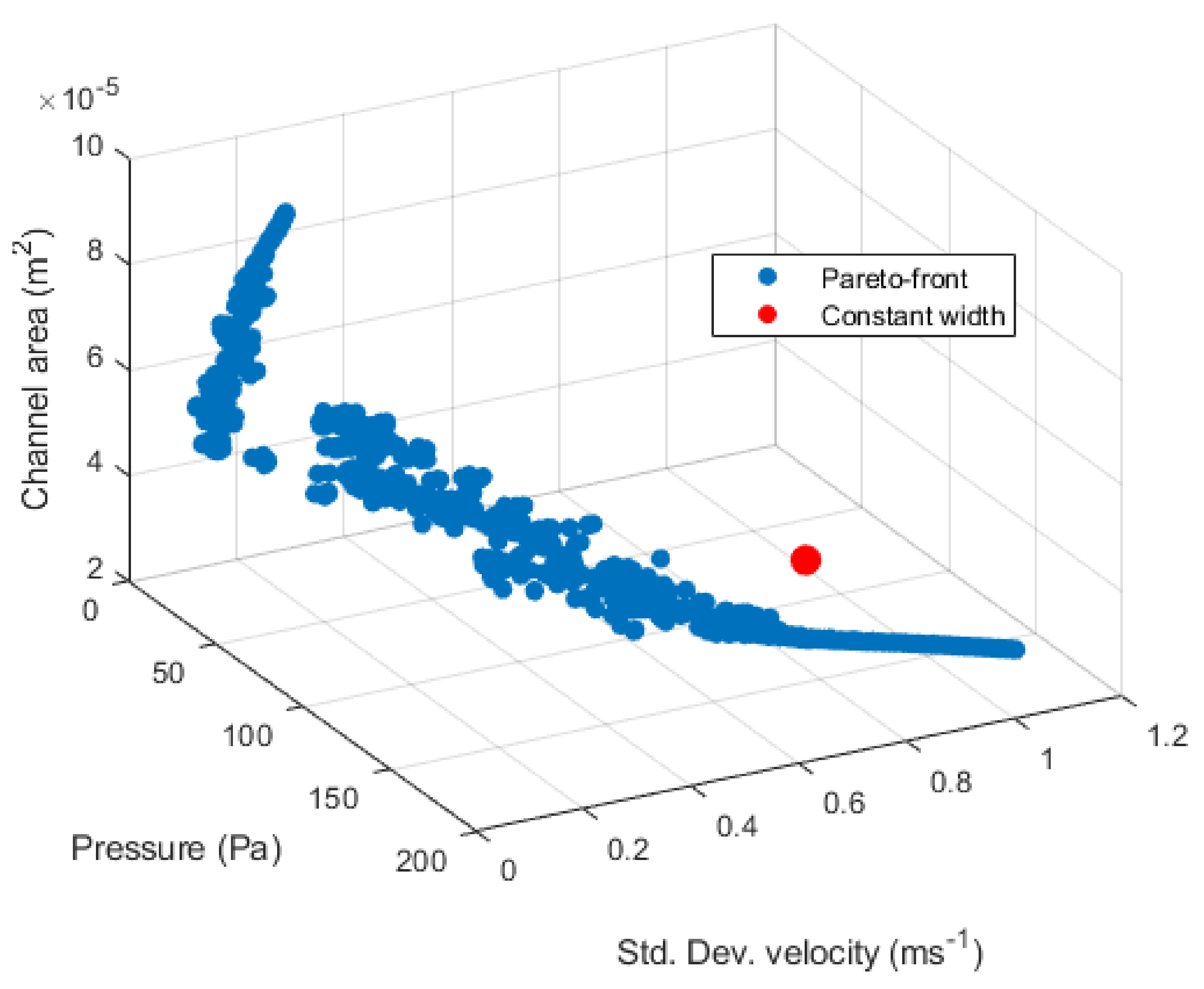
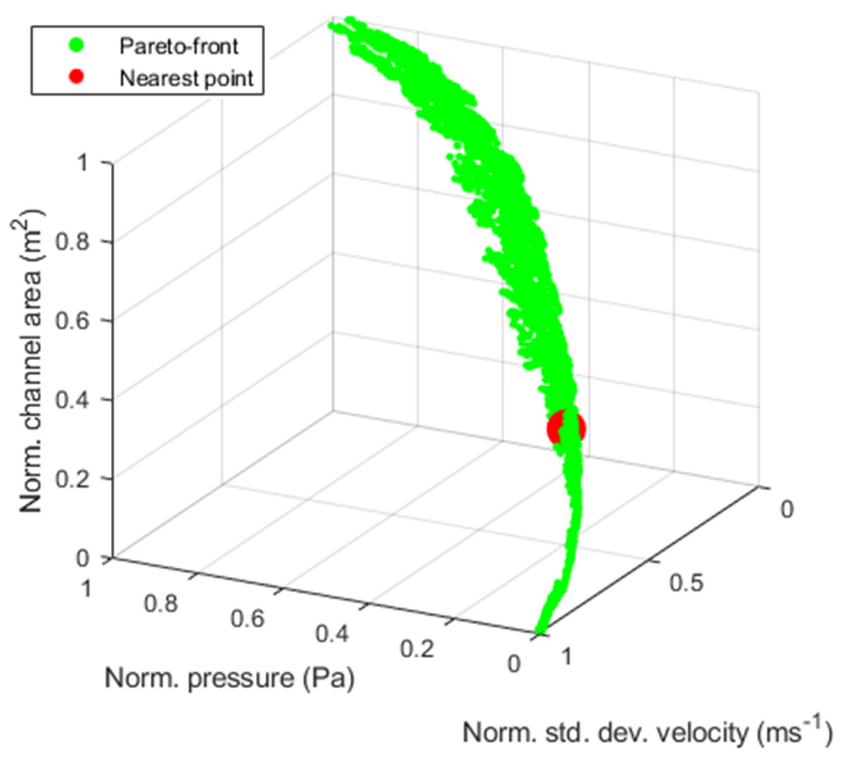
The input to the problem was the widths of all the channel. This means the problem was a multivariable problem—having several decision variables. Some of the objectives mentioned are in direct conflict with one another: improving the pressure drop with wider channels directly leads to reduced area available for conduction and a wide range of flow velocities. Channels with uniform width may be easy to manufacture, but the flow velocities would be non-uniform. Such problems are classified as multiobjective optimization problems (MOOP). It is not possible to simultaneously optimize each objective. Rather, in a MOOP, the designer obtains a Pareto-front of solutions, which includes the extreme values for each objective. Then, some higher-level information is applied to select one solution with the best tradeoff to implement. Such an approach gives the designer flexibility as a wide range of solutions is available.

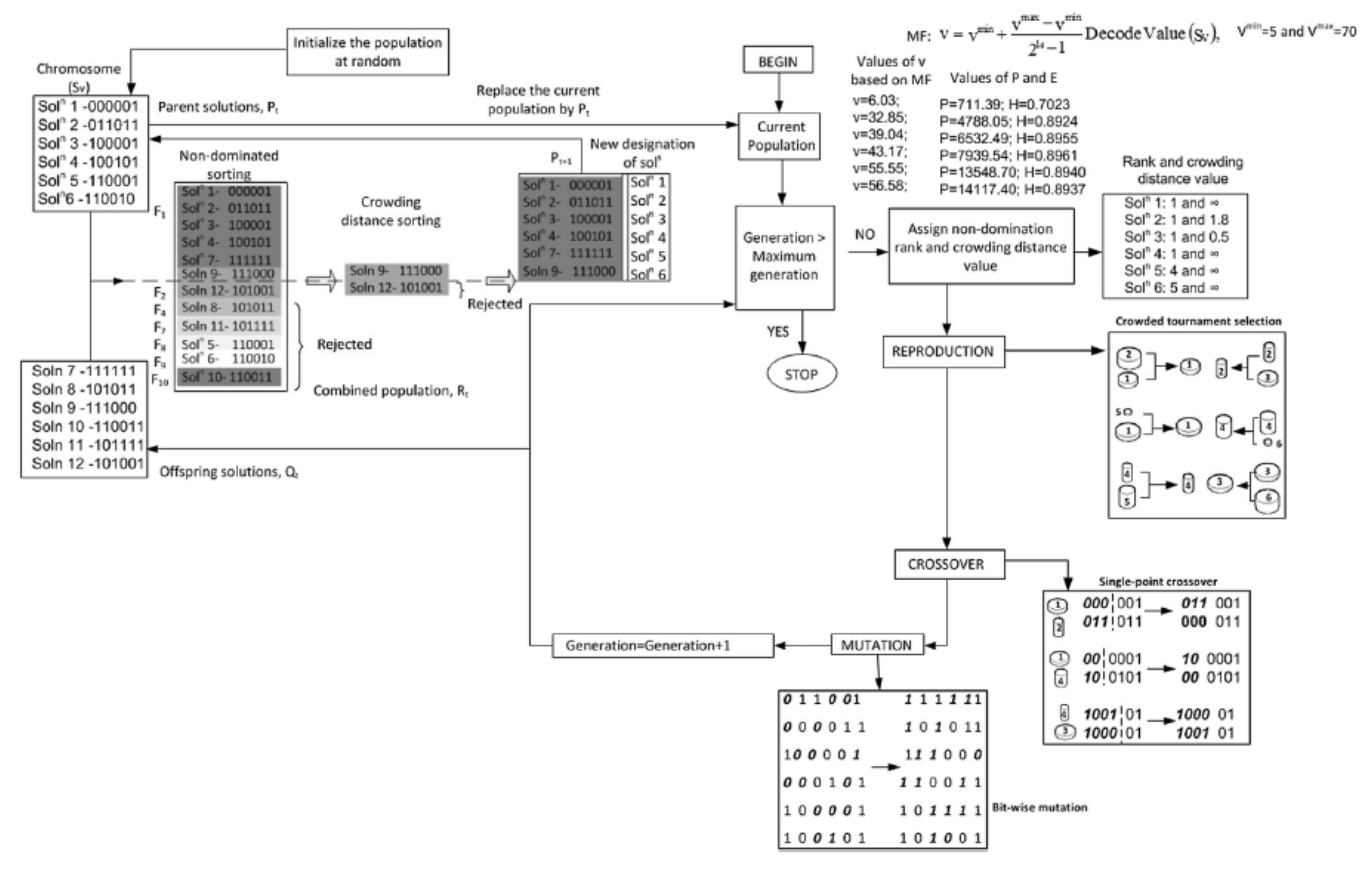
In this study, a genetic algorithm was used to solve the problem. A genetic algorithm (GA) is an optimization tool that mimics the principles of genetics and natural selection. They operate by applying the principle of “survival of the fittest” on a population of candidate solutions to successively produce better solutions through each generation. Multiobjective Gas (MOGA) area a class of tools based on Gas that are used find a set of solutions based on the principle of non-domination. The closer this set of solutions is to the true Pareto-optimal front, the better the algorithm. A MOGA was used in this study as it produces a solution set that is a good approximation of the Pareto-front thereby effectively solving the MOOP. Local minima are also avoided. Furthermore, it gives solutions that are distributed throughout the front, leading to a wide choice from which the designer can pick a solution that best fits their need. To do this, a non-dominated sorting genetic algorithm, NSGA-II [17], one of the most widely used GA, was adopted. Figure 2 shows a step-by-step procedure for NSGA-II for a problem with two objective functions and one decision variable, which can be easily adopted for an arbitrary number of objectives and decision variables. A detailed description with a practical example can be found in Reference [18].

Optimization of fuel cell flow fields is not well studied in the literature and there are even fewer studies involving multiobjective optimization. Kizilova et al. [19] used the principle of minimum entropy generation to optimize fractal-like flow channel designs for PEMFCs. A simplified 1D model was found to give results of comparable accuracy to a 3D model. Zhang et al. [20] looked at the serpentine flow field with three different flow rates and four different land widths. The highest flow rate gave the best performance. Similarly, the larger the land width, the better the performance. Pumping power was found to significantly affect all these results. Similarly, Luo et al. [21] looked at adding rib grooves to the serpentine flow field channels. A diminishing rate of return was found with increasing rate of rib grooves. Li et al. [22] was a study that used a GA coupled with a CFD (computational fluid dynamics) package to optimize a blocked channel design. The block heights in the channels were the decision variables. Only 20 generations were needed to achieve convergence, most likely because only one channel was analyzed. Liu et al. [23] used a genetic algorithm to solve a MOOP whose objectives were maximizing energy efficiency and output power of the fuel cell. The operating conditions and channel dimensions were the decision variables. Sohani et al. [24] also optimized the operating conditions, i.e., pressure, temperature, stoichiometry, etc., to find the best efficiency, economics, size, and environmental impact. The results were presented for various applications. Xie et al. [25] also optimized channel geometry to improve output power and reduce power consumption. None of the studies in the literature considered the objective functions mentioned here simultaneously while optimizing the geometry of an entire flow field.

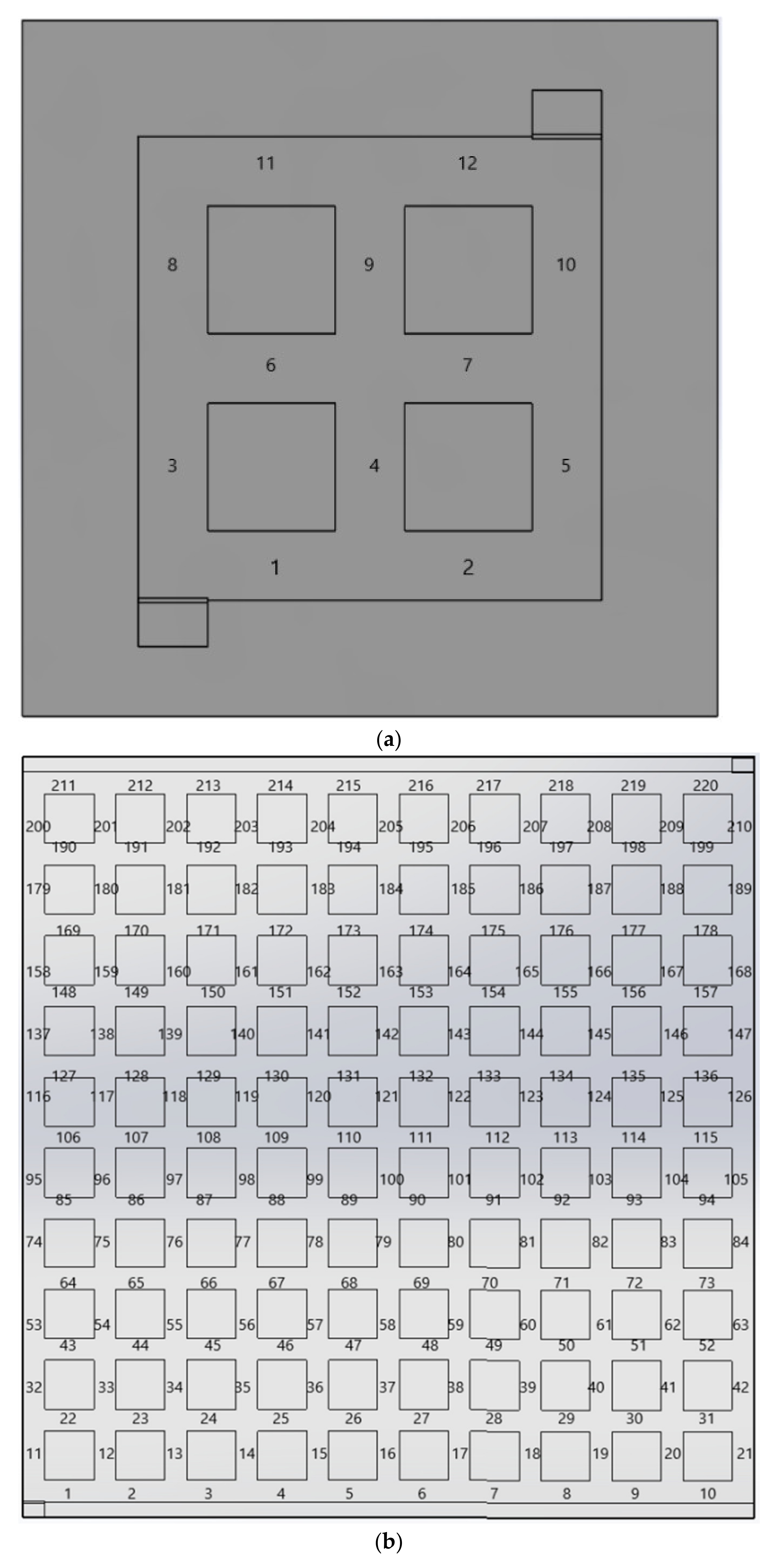
The following section presents the flow field model used for optimization. A pin-type flow field was used as an example. The section after that presents optimization results.

3. Pin-Type Flow Channel Model

3.1. Schematics and Assumptions

The pin-type flow field was used to demonstrate the MOOP regarding flow fields. The method can be extended to any flow field geometry as long as the following assumptions [16] hold.

• The flow is laminar.
• The reactant gases are viscous and incompressible.
• A constant resistance coefficient, which is estimated empirically, exists at each junction.
• Reactants are not consumed. The goal of this study is to examine flow optimization. In typical fuel cell flow fields, less than half the supplied reactants are consumed. Most of the gases pass through and are recycled. Consumption can be added in future studies.

Figure 3 shows a basic schematic with all the important parameters labeled. A general configuration is shown where the flow field has M × N nodes. The number of channels in such a configuration is 2MN − M − N. In this study, similar to [16], the cases for 3 × 3 (12 channels) and 11 × 11 (220 channels) were examined. These are representative of experimental flow fields found in the literature. Figure 3 shows the inlet and outlet circled as well as the direction of flow. Three types of junction or node exist: cross-junction with two channels flowing in and two flowing out; L-corner with one in and one out; and T-junction with either one or two channels flowing in and one flowing out or one flowing in and two flowing out. Figure 4 shows the two flow fields analyzed here with the channels labeled. These labels were used in the flow simulations. In Reference [16], a matrix-style naming convention was used where each node was denoted by its row and column index: i, j. Each channel was then denoted by its initial and terminal nodes: (ij). This makes it easy to generalize equations for an M × N system. The pressure for each node is an unknown and the flow rate across each channel is also an unknown. By using Equation (1) for pressure drops across each channel and continuity or mass balance at each junction, there are enough equations to solve for all unknowns. However, there is a tremendous amount of tedious algebra involved in rearranging hundreds of linear equations so they can be entered into a matrix equation solver. In this study, a different method was adopted as is explained below.

3.2. Model Equations and Solution Approach

The flow model used in [16] is summarized here. The pressure loss across any channel is given by Equation (1). The hydraulic diameter is given by:

$$D_i=\frac{4A_i}{P_{c,i}}=\frac{2w_i{d}_i}{w_i+d_i}$$

(9)

where A_i is the area of the channel, P_c,i is the wetted perimeter of the channel, w_i is the channel width, and d_i is the depth. The volumetric flow rate is:

$$q_i=v_i{A}_i$$

(10)

where v_i is the average flow velocity in the channel. Equation (1) can be written in terms of a flow resistance, R_i.

$$p_i=R_i{q}_i$$

(11)

To take the pressure losses at the conjunction of channel segments into account, a constant resistance coefficient of 3.6e5 [26], R_c, was introduced to the flow resistance equation.

$$R_i=\frac{128\mu L_i}{\pi D_i^4}+R_c$$

(12)

For any of the three types of nodes mentioned, continuity gives:

$${\displaystyle \sum }_i{q}_i=0$$

(13)

The inlet flow rate (q_in) and outlet flow rate (q_out) are equal. In Reference [16], Equations (11) and (12) were combined and substituted into Equation (13) to give a system of 3 × 3 or 11 × 11 linear equations that, when solved, give the pressure at each node. As mentioned, a lot of tedious algebra is involved in entering these equations. Furthermore, if a new geometry is designed, the whole process has to be repeated. In this study, a different approach, one that is more amenable to design changes, was adopted. The decision variables or inputs to the MOGA were the channel widths. In Equation (10), the volumetric flow rate in a given channel is proportionate to the average flow velocity and the cross-sectional area. Since all the channels have the same depth, the flow rate is proportional only to the channel width. If optimization of the channel widths produces uniform flow velocities, then the flow rate of a channel only depends on the width of that channel. Thus, the widths were used to guess the flow rate of each channel. The continuity condition at various junctions was used as a constraint to ensure that realistic flow rates were obtained by the algorithm. Then, Equation (11) was used to calculate the pressure drop and 10 to obtain velocities. This approach made it relatively easier to scale from 3 × 3 to 11 × 11 and beyond.

3.3. Decision Variables and Objective Functions

The decision variables were the channel widths. For the 3 × 3 system, 12 variables were needed. For the 11 × 11 system, 220 were needed. The lower and upper limits were 0.5 mm and 2.2 mm, similar to [16]. Four objective functions were used. The first objective was to minimize the pressure drop. This is a complex calculation for the geometry that was analyzed, so the sum of the pressure drop for each channel was considered as the objective.

$$\min P\left(w_i\right)=\sum p_i$$

(14)

Virtually every channel would have a slightly different pressure drop because the MOGA would pick a slightly different width based on guided random chance. The second objective was to minimize the standard deviation of the flow velocities.

$$\min S\left(w_i\right)=\sqrt{\frac{\sum {\left(v_i-\overline{v}\right)}^2}{2MN-M-N}}$$

(15)

where $\overline{v}$ is the average flow velocity. The third objective was to minimize the total channel area, thereby maximizing the land or rib conduction area. Figure 5 shows a typical rib or land segment. It is a square of side L. The algorithm picks the channel widths and all four are expected to be different. Equation (16) shows the calculation of the channel area for a typical segment.

$$\min A_{chan}\left(w_i\right)={\displaystyle \sum }_i{L}^2-\left(L-\frac{w_1+w_2}{2}\right)\left(L-\frac{w_3+w_4}{2}\right)$$

(16)

It must be noted that for the peripheral channels, this formula was appropriately modified to account for the different geometry. The fourth objective was to minimize the manufacturing cost.

$$\min M\left(w_i\right)=\sum L{w}_i{}^n$$

(17)

As mentioned previously, this formula accounts for the amount of material to be removed from the channels with n = 2. Another way to think about this is to consider it as the cost of design and prototyping (e.g., programming a CNC machine). It does not necessarily apply to mass production. Different values of n were studied. Future studies can consider other functions. In Reference [16], an area constraint was used to ensure at least 40% of the total flow field area was available for conduction. In this study, this constraint was not necessary as area of conduction is an objective.

Table 1. Flow parameters.

Channel length, L, mm	5
Channel depth, mm	1
Fluid viscosity, kg/m/s	9.93 × 10−6
Active area (3 × 3), mm2	10 × 10
Active area (11 × 11), mm2	50 × 50
Inlet pressure (kPa)	101,325
Inlet flow rate (m3/s)	4.6 × 10−6

lists the flow parameters that were used and

Table 2. Genetic algorithm parameters.

Algorithm	NSGA-II
Number of objectives	2–4
Number of decision variables	12–220
Lower/upper limits, w, mm	[0.5, 2.2]
Population size	1× 104
Number of generations	1× 103
Crossover probability	0.9
Mutation probability	0.01
Tournament size	2
Selection type	Crowded tournament *

* fronts are ranked; if equal, crowding distance is used.

lists the GA parameters. Wherever possible, parameters have been chosen to match the literature. The large population size for NSGA-II reflects the large number of decision variables.

4. Results

This section details the results of various studies pertaining to optimization of the pin-type flow field using MOGA.

Table 3. Computational fluid dynamics (CFD) parameters.

System of units	Metric
Analysis type	Internal
Fluid	Hydrogen gas
Wall thermal condition	Adiabatic
Roughness	0 μm
Inlet condition	Mass flux
Outlet condition	Pressure (101,325 Pa)
Temperature	293 K
Number of cells	353,780
Iterations (average)	148
Number of cores	4
CPU time (average)	17 m 12 s

shows the CFD parameters used for all simulations.

4.1. Finding Murray’s Law

The 3 × 3 system in Figure 4 was used to demonstrate that NSGA-II can find optimized channel widths in accordance with Murray’s Law. Only two objectives were considered for this demonstration, which are the same as the ones implicit in Murray’s Law: pressure and manufacturing cost. In Equation (4), these two quantities are added. Thus, minimizing the function involves minimizing the sum of these two objectives. NSGA-II provides a Pareto-front where both objectives range in value. If the two objective values are added, the lowest total represents the minimum value of the function. Murray’s Law of flow splits was applied to the channel widths that produced this minimum solution. As per Figure 4, the four junctions analyzed were at the intersection of channels 1–2–4, 3–6–8, 5–7–10, and 11–9–12. If Murray’s Law was followed perfectly, then the difference between the cube of the parent channel’s hydraulic diameter and the sum of the cubes of the daughter channels’ hydraulic diameters would be zero. Figure 6 shows a plot of the average deviation from zero averaged over the four junctions considered. The deviation is plotted against the sum of the two objectives for each solution (1000 solutions considered for demonstration purposes). If NSGA-II was successfully picking channel widths in accordance with Murray’s Law, then a linear, monotonically increasing relationship would be expected: the lower the function value, the lower the average deviation. This is the trend that is seen in the plot. The R²-value is 0.9348, implying an excellent fit. This, it can be concluded that the algorithm successfully picks channel widths in accordance with Murray’s Law. This is important and useful because no a priori information about the cube relation is programmed and no information about the flow rates is provided either.

4.2. Flow Split at T-Junctions

The pin-type flow field has three types of junction. The flow split or fraction of flow from the parent channel that ends up in the daughter channel(s) for L-corners and cross-junctions is straightforward. For L-corners, no flow split happens. For cross-junctions, symmetry dictates the fraction. Of course, with a MOGA, there is no guarantee that the daughter channels will be symmetric, but the channel widths can be used along with the continuity condition. At T-junctions, the 90-degree angle makes it necessary to closely examine if the flow split is truly a function of the channel widths. A CFD simulation was run with varying widths for the branch. The results are shown in Figure 7. Note that the parent channel’s width was maintained the same. The x-axis displays the branch channel width as a fraction of the parent channel width. As the branch channel width increases, so does its flow and the flow in the parent channel correspondingly decreases. The flow split was found to vary almost perfectly linearly with an R²-value of 0.99. Thus, the flow model described in Section 3 could be expected to produce accurate results.

4.3. Conventional Optimization vs. Multiobjective Genetic Algorithm (MOGA)

Before analyzing MOGA results, the advantage of MOGA is demonstrated by comparing to conventional, single-objective optimization (SOO). A constrained non-linear optimization was used since multiple variables were involved. The objective selected was standard deviation of flow velocities, just like in [16]. Here itself lies the main weakness of conventional optimization: only one variable can be optimized—the rest must be treated as constraints or ignored.

Table 4. Comparison of optimization algorithms.

Algorithm	SOO	MOGA	%
Std. Dev. velocity (ms−1)	1.98 × 10−3	9.6 × 10−4	51.5
Pressure (Pa)	37.1	36.9	0.5
Manufacturability (× 109 m3)	154	154	0
Channel area (m2)	6.67 × 10−5	6.67 × 10−5	0

shows the results. The percent column shows how much larger SOO is compared to MOGA, which is a way of quantifying how much worse it performs as the objective is to minimize these objectives. The main objective, standard deviation of flow velocities, is 51.5% worse. This demonstrates the other weakness of conventional search algorithms. Genetic algorithms search the multivariable decision space very efficiently to produce good solutions. Traditional algorithms can become stuck in local minima. For the other three objectives, MOGA is the same as or better than SOO. Note that for SOO, the other three objectives were computed as constraints and not actively minimized as only one objective can be minimized in SOO. MOGA does not suffer from this limitation. As will be demonstrated in the next section, a Pareto front of the entire non-dominated objective space is presented to the optimizer and a suitable solution can be chosen based on some higher-level decision-making.

4.4. MOGA Results for 3 × 3 Design

The 3 × 3 flow field was analyzed first using the described model and MOGA settings. All four objectives were programmed, and the results can be seen in Figure 8. It shows the Pareto-front that was obtained. As four objectives are involved, a Pareto-surface is obtained. The fourth objective is shown using a colorbar. In Figure 8a, the area is represented with the colorbar. If Figure 8b, to show a different view of the plot, the manufacturability (×10⁹) is represented with the colorbar. A classic front for a min-min-min-min problem is obtained, where its only vertex tends towards the origin. To determine the relationships between individual objectives, they were plotted two at a time. It was found that the manufacturability (M) and the area (A) were correlated; minimizing one always minimized the other. Thus, only the pressure, area, and standard deviation of the flow velocities were considered for the rest of the study.

Accordingly, Figure 9 shows the data from Figure 8 plotted again, but only with the three objectives considered. The objectives were also evaluated for constant channel widths (0.6 mm) as an example and the objective values are plotted in red. This non-optimized solution clearly stands out from the Pareto-front. It demonstrates the efficacy of the proposed MOGA approach to flow field design. Not only is it dominated by the front, it is located much further away from the ideal point, which is the origin (0,0,0) for a min-min-min problem, than the rest of the front.

4.5. MOGA Results for 11 × 11 Design

The same simulation was run again for the 11 × 11 flow field. The Pareto-front is shown in Figure 10. The front has a similar shape as the front in Figure 9. However, the ranges are different as expected. The flow velocities are much more uniform as demonstrated by the narrower range of standard deviation of flow velocities. Even though there are more channels in this design compared to the 3 × 3 design, the pressure drop ends up in a narrower range. The reason this happens is because the flow rate is maintained at the same value for both designs, meaning there is a lot more area for the same flow. Thus, the average flow rate is smaller in any given channel and so the pressure drop is smaller as well. The same explanation can be extended to the flow velocities. Given the larger area, the flow velocities are lower in general, so the standard deviations also end up low.

The comparison between the two designs is not the goal. Rather, it is the comparison between the optimized and unoptimized designs that provides the greatest insight. This is explored in the next section.

4.6. Computational Fluid Dynamics (CFD) Results for 3 × 3 Design

The flow performance of two variations of the 3 × 3 design was analyzed for comparison and to validate the GA results. The first variation was the one in Figure 4a, the unoptimized design. The channel width was 1.5 mm for each channel. The second variation used channel widths from the MOGA results. A sample solution from the Pareto-front in Figure 9 was selected. The 12 widths were entered in Microsoft Excel. The drawing of the flow field in SolidWorks was edited to use parameters drawn from a design table. This design table was linked to the Excel spreadsheet, making it easy to change the design with different GA solutions. This approach was especially useful for the 11 × 11 design with 220 widths. CFD simulations were run using the parameters in Table 3.

Figure 11 shows the velocity contour plot. The unoptimized design has a maximum velocity about 1.25% higher. This is a marginal increase, but the narrower inlet and outlet are expected to produce a higher flow velocity. Generally, it is desirable to have the lowest possible flow velocity so the gases can diffuse out of the flow field into the electrolyte. However, uniform flow velocities in all channels is the ultimate goal. The more interesting result that shows the benefit of the MOGA design is the inner channels: 4, 6, 7, and 9. In the unoptimized design, the velocity is between 1.1 m/s and 1.6 m/s. In the MOGA design, it is closer to 2.4 m/s. This would greatly improve the fuel cell’s performance by avoiding a massive dead zone in the middle of the flow field. More importantly, the outer channels (2, 5, 8, and 11) have a higher velocity as well. Whereas in the unoptimized design, there are zones of nearly zero velocity, this is reduced in the MOGA design. Thus, the performance of the entire flow field would be better. The pressure objective function has a value of 23 for the unoptimized design compared to 13.3 for the MOGA design, about 42% lower. However, the area is about 6% higher. The standard deviation of the velocities is 0.35 compared to 0.021 for the MOGA design, which is 94% lower. These results are very similar to those reported by [16]. In this study, only one solution was found as there was only one objective. This solution is part of the front in Figure 9, one of the extreme values. Thus, it is seen that one of the three objectives is 6% better for the unoptimized design, but the other two are 42% and 94% better for the optimized one.

4.7. CFD Results for 11 × 11 Design

Repeating the process for the 11 × 11 design yielded Figure 12. This type of flow field is more representative of a full-size fuel cell flow field. A similar trend is seen as the 3 × 3 design. Note that the upper limit has been capped at 2 m/s, so more details can be noted. The maximum velocity in the unoptimized design is 4.98 m/s and in the MOGA design, it is 4.94 m/s, a 0.8% difference. The real efficacy, once again, is seen within the outer channels. In Figure 12a, the channels towards the top left and bottom right have a near-zero velocity, a steep decline from the inlet and outlet velocities. The velocity also drops off towards the center region. This uneven distribution of reactants and removal of products would lead to a deterioration in the performance and lifespan of the fuel cell. For the MOGA design, several of the channels in the middle have non-zero velocities. None of the channels appear to have a completely zero velocity, which is excellent for performance. The pressure objective function has a value of 115 for the unoptimized design compared to 223 for the MOGA design, about 94% higher. However, the MOGA area is about 27% higher. The standard deviation of the velocities is 0.253 compared to 0.108 for the MOGA design, which is 57% lower. This is not unexpected. Considering the number of generations of branches, almost all of the lowest branches have the same channel width of 0.5 mm. This implies that the algorithm would prefer to choose a lower width if it was available, but 0.5 mm was set as the lower limit based on potential manufacturing limitations. Even with this type of limit, two of the three objectives are improved. It must be noted that, given the nature of multiobjective optimization, choosing a different solution would result in different values for the objective functions. This different solution might have a lower pressure, but also a lower area. Overall, it is clear that MOGA solutions produce much more uniform flow in the pin-type flow field.

4.8. Sensitivity of Manufacturability Objective

Equation (8) gives the total pumping effort. The exponent, n, was taken to be 2 (Equation (17)). This proposes that the manufacturability is proportional to the volume of material that needs to be removed. However, as discussed in Section 2.1, physiological studies have found the cubic relation in Equation (7) to vary from 2.33 to 3.006. As was stated in Section 2.1, the exponent of branching in Murray’s Law is (n + 4)/2. For example, when n = 2, the expected exponent of 3 is obtained. If however, the data suggests the exponent should be 2.33 instead of 3, that would imply n to be 0.66. This low value may be feasible in a biological system, but may not be in a man-made system.

The 3 × 3 flow field simulation was run with different values of n: 1.5, 2, and 3. Only two objectives were considered to make plotting them easier. The results are in Figure 13. Note that the normalized values of the objective functions were plotted. This was necessary as the different values of n produced values of manufacturability that were different by orders of magnitude. Of interest here is not the value of the objectives, but only the shape of the front. Thus, the most equitable comparison can be afforded by normalizing all objective values. The most notable aspect of the shape of the fronts in Figure 13 is that as n increases, the curvature is sharper. The ideal point for a min-min problem is the origin (0,0). The highest n value gets closest to this point. However, this also corresponds to the highest manufacturability cost. Note that the lowest pressure on all three fronts converges to some common minimum value, meaning is it not possible to drop below a certain minimum pressure. This corresponds to the widest channel, the upper limit of the search space. It was the same for all three cases, so it has the same extreme value, and is not dependent on n. What is interesting, perhaps, is the fact that as the manufacturability improves (decreases) and pressure increases, it does so in the slowest manner for the highest n value. Beyond this, a physical interpretation is not sensible.

The metabolic coefficient in Murray’s Law is a constant for a given system. In this study, the channel length served this role. Finding the precise value can be challenging and the literature suggests a variety of values for different cases. For example, The work in [27] proposes values for pig tissue. No matter what value is used, the results are not expected to change as it is just a constant scaling coefficient in the equation.

4.9. Selection of an Optimal Solution

The process of how an optimal solution could be selected is presented here. Once a Pareto-front of solutions is obtained, it is not possible to choose one non-dominated solution over another as neither one gives a clear advantage, namely improving all objectives simultaneously. Thus, some higher-level information must be used, commonly referred to as multi-criteria decision-making techniques (MCDM). One MCDM approach is the ideal point method [28]. Here, the optimizer picks an optimal solution that has the least geometric distance to some reference point, like the ideal point. For a min-min-min problem like the current one, the ideal point is the origin (0,0,0). In practice, no solution will produce these values. However, a point on the Pareto-front that is nearest to this point may be considered the most optimal. Again, normalized fronts were used, and the result is shown in Figure 14. The objective values corresponding to this point are (90.6 Pa, 0.16 ms⁻¹, 9.59 × 10⁻⁴ m²). The location of the nearest point on the front is expected: physically nearest to the origin. Comparing the objective values to the original front in Figure 10, the values are close to the midpoint of each individual objective value’s range, which represents the best tradeoff.

5. Fuel Cell Performance

CFD software packages have been used extensively in the literature to test the performance of various flow field designs used in PEMFCs. Several studies have derived inspiration from Murray’s law and compared CFD simulations to experimental results [8,9,10,16]. This section uses a similar approach to provide a quick, cost-effective way to compare the performance of the proposed design in a fuel cell. The same CFD settings in Table 3 were used. The additional FC-specific parameters were from [16] and are summarized in

Table 5. Fuel cell CFD parameters.

Anode stoichiometry	2
Cathode stoichiometry	2
Relative humidity at anode (%)	0
Relative humidity at cathode (%)	100
Charge transfer coefficient at anode	1
Charge transfer coefficient at cathode	1
Concentration exponent at anode	0.5
Concentration exponent at cathode	1.0
Pore blockage saturation exponent	2.0
Open circuit voltage (V)	0.98
H2 diffusivity (m2/s)	8.0 × 10−5
O2 diffusivity (m2/s)	2.0 × 10−5
H2O diffusivity (m2/s)	5.0 × 10−5
Membrane equivalent weight (kg/kmol)	1100
Catalyst layer surface-to-volume ratio (1/m)	1.25 × 107
GDL electric conductivity (1/Ωm)	280
GDL porosity	0.82
GDL wall contact angle (deg)	110
GDL viscous resistance at anode (1/m2)	1.0 × 1012
GDL viscous resistance at cathode (1/m2)	3.86 × 1012
Bipolar plate electric conductivity (1/Ωm)	92,600

. Note the GDL refers to the gas diffusion layer of the fuel cell.

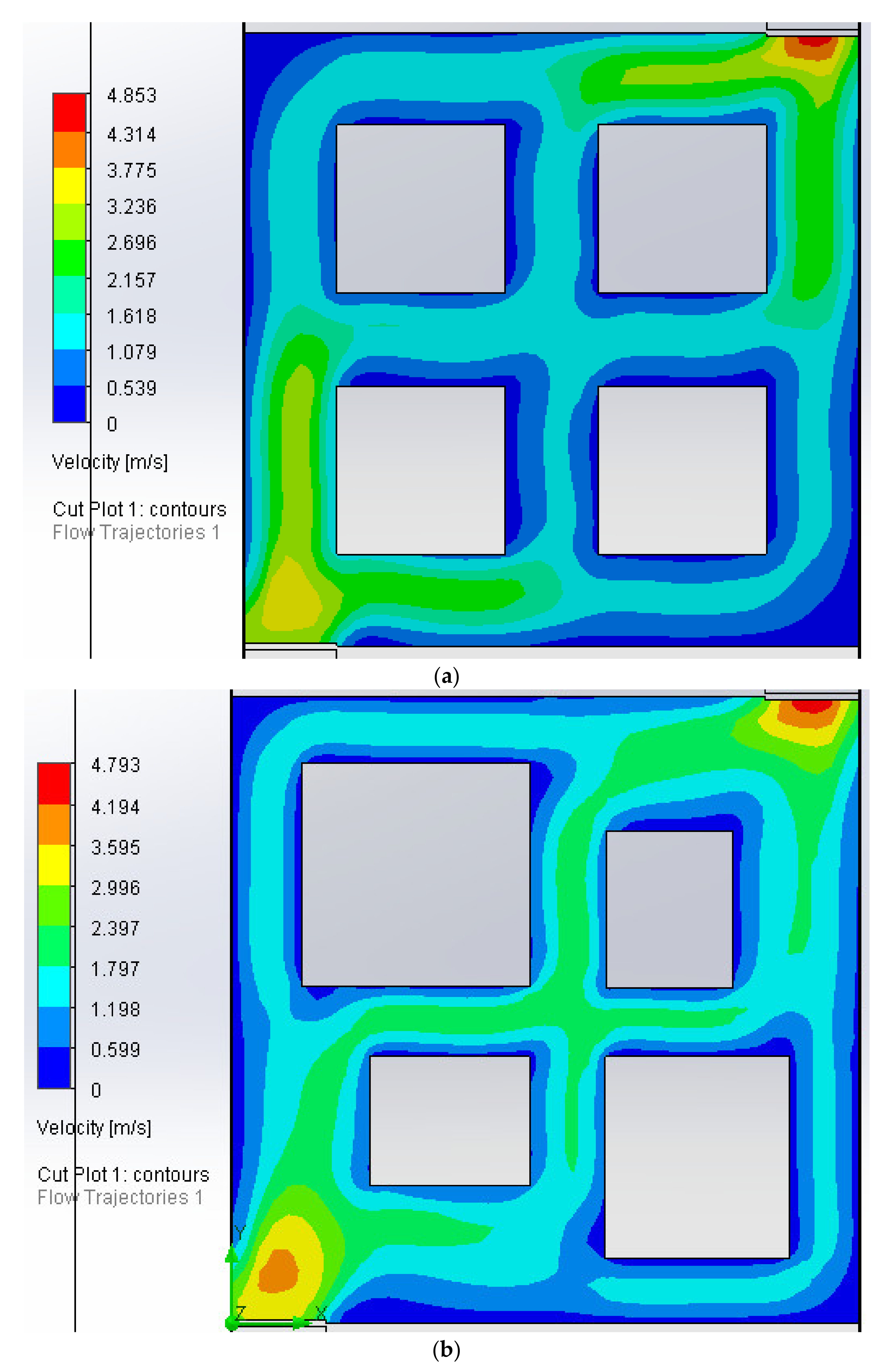
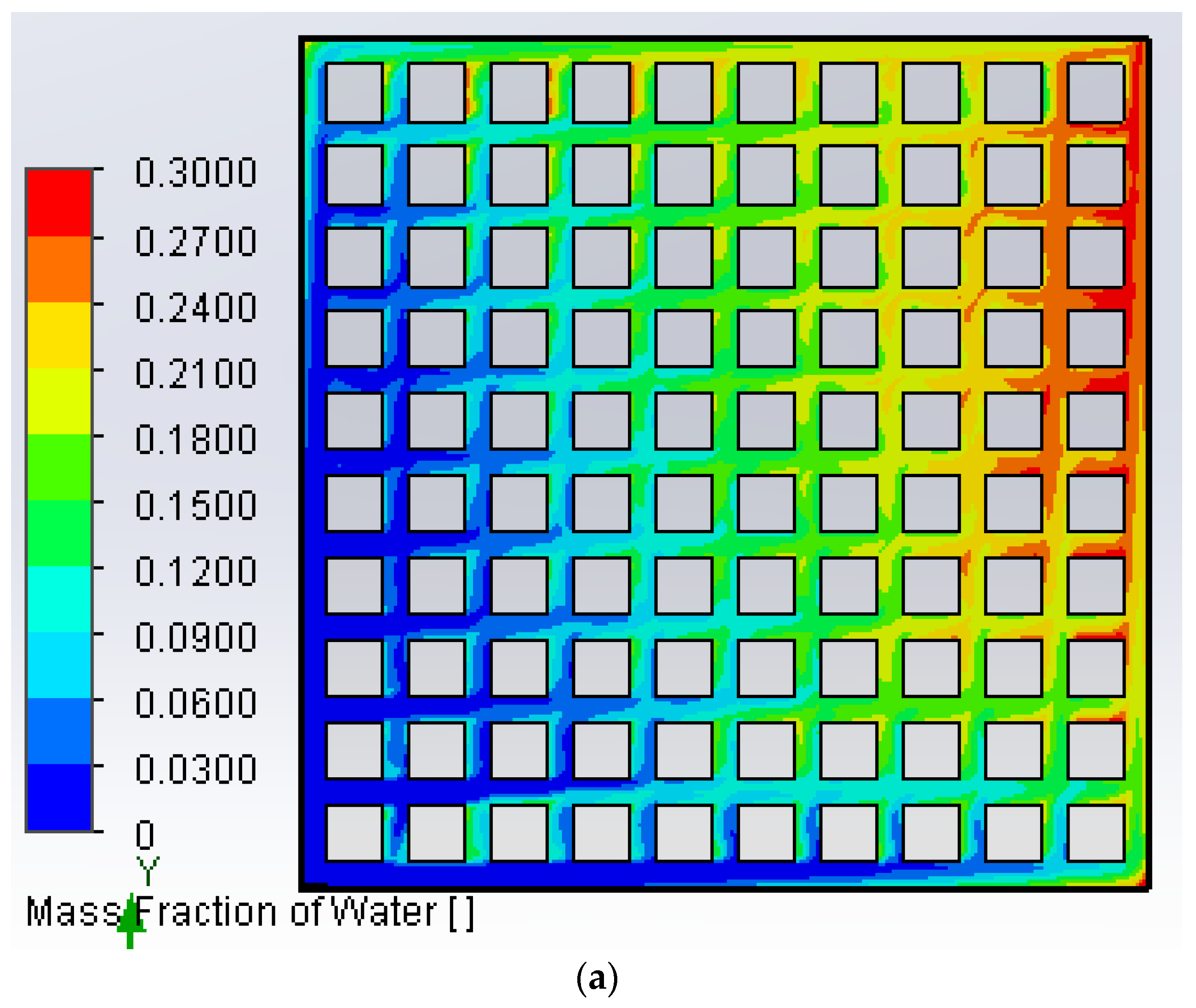
Figure 15 shows flow results. The mass fraction of water is shown because the aim of this study is to investigate the performance of nature-inspired designs using Murray’s Law. Water is a byproduct in PEMFC operation and has been shown to be a significant limiting factor at high current densities [10]. Thus, removal of water is a critical determining factor in selecting effective designs. Note that in Figure 15, the upper limit is set to 0.3 in order to glean greater details in the results; mass fraction of water is not expected to be significantly close to 1.0 as most of the fluid in the channel is the reactant gas. As can be seen, the non-optimized design has a higher mass fraction in several regions, particularly in the corners opposite the inlet/outlet. Comparatively, the MOGA design does a better job at removing water. These results are generally consistent with previous studies on pin-type designs. Guo et al. [16] found a similar issue with water saturation in the corners.

It is difficult to quantify the difference. If the mass fraction at every computational node in the flow channels is averaged, the value for the unoptimized design is 0.1712 and for the MOGA design it is 0.1564, about 9% lower. Heck et al. [10] came to similar conclusions on nature-inspired designs being better at water management. These results are also consistent with the flow simulation results in Figure 12. The peak current density in the unoptimized design was 0.76 A/cm² and for the MOGA design it was 1.35 A/cm². This further confirms the efficacy of the MOGA design and matches results found in [16].

6. Conclusions

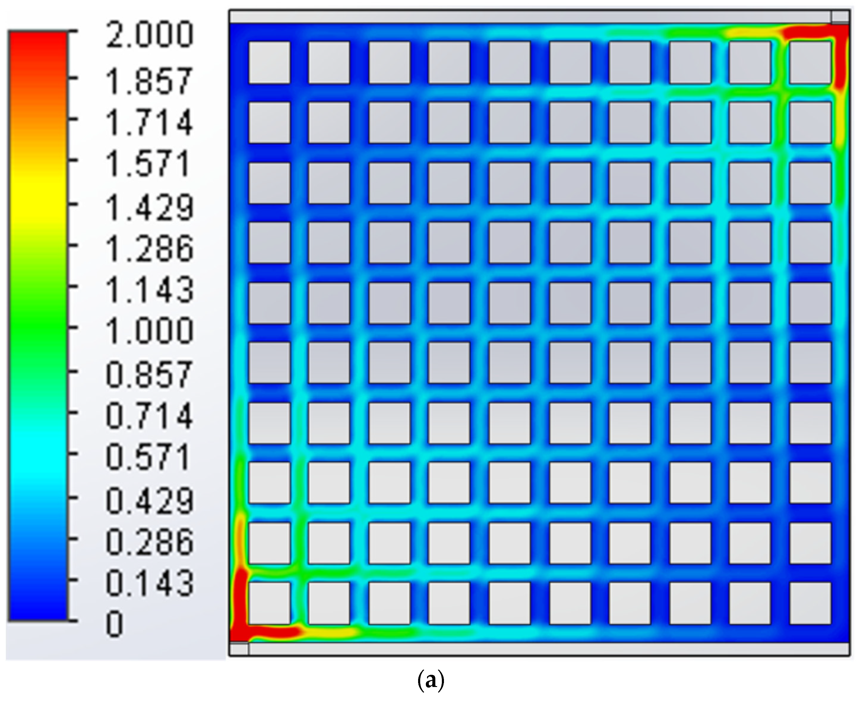
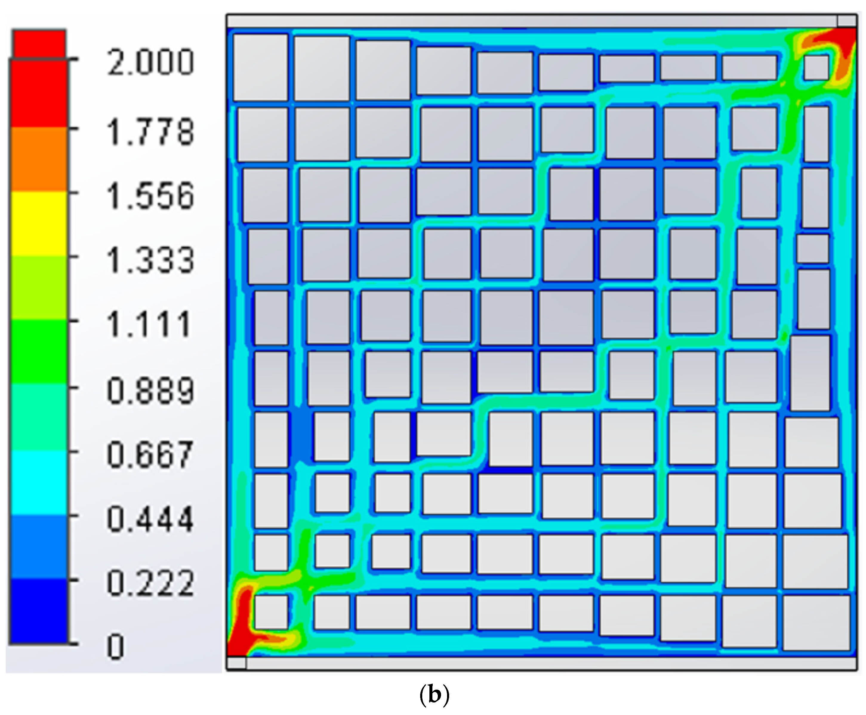
The present work examines the applicability of Murray’s Law to flow fields for fuel cells and other flow devices. To design effective flow fields, the problem was cast as a multiobjective optimization problem with conflicting objectives. Four objectives were considered and applied to the pin-type flow field. Two geometric scales were analyzed, the 3 × 3 and the 11 × 11 design. Pareto-fronts were obtained. One solution from these fronts was picked for illustrative purposes. Then, using the channel widths produced by NSGA-II, the flow fields were modeled in SolidWorks and CFD simulations were performed. The optimized designs were compared with their unoptimized counterparts, those with constant channel widths. In both cases, the optimized designs had a lower maximum flow velocity and the standard deviation of the flow velocities in the channels was lower, 94% and 57% lower for the 3 × 3 and the 11 × 11 designs, respectively. These were found to be similar to existing studies. The nearest point method was used to demonstrate how one solution from a front of non-dominated solutions may be selected. Finally, CFD fuel cell simulations further confirmed the performance benefits of the MOGA design. Future studies can consider other geometries and consider reactant consumption. Branching ratios and frequency can also be studied.

References

1. Tsuchiya, H.; Kobayashi, O. Mass production cost of PEM fuel cell by learning curve. Int. J. Hydrogen Energy 2004, 29, 985–990. [Google Scholar] [CrossRef]
2. Li, X.; Sabir, I. Review of bipolar plates in PEM fuel cells: Flow-field designs. Int. J. Hydrogen Energy 2005, 30, 359–371. [Google Scholar] [CrossRef]
3. Iranzo, A.; Arredondo, C.H.; Kannan, A.M.; Rosa, F. Biomimetic flow fields for proton exchange membrane fuel cells: A review of design trends. Energy 2020, 190, 116435. [Google Scholar] [CrossRef]
4. Kloess, J.P.; Wang, X.; Liu, J.; Shi, Z.; Guessous, L. Investigation of bio-inspired flow channel designs for bipolar plates in proton exchange membrane fuel cells. J. Power Sources 2009, 188, 132–140. [Google Scholar] [CrossRef]
5. Arvay, A.; French, J.; Wanga, J.-C.; Peng, X.-H.; Kannan, A.M. Nature inspired flow field designs for proton exchange membrane fuel cell. Int. J. Hydrogen Energy 2013, 38, 3717–3726. [Google Scholar] [CrossRef]
6. Wang, C.T.; Hu, Y.C.; Zheng, P.L. Novel biometric flow slab design for improvement of PEMFC performance. Appl. Energy 2010, 87, 1366–1375. [Google Scholar] [CrossRef]
7. Murray, C.D. The physiological principle of minimum work. I. The vascular system and the cost of blood volume. Physiology 1926, 12, 207–214. [Google Scholar] [CrossRef] [PubMed] [Green Version]
8. Guo, N.; Leu, M.C.; Koylu, U.O. Bio-inspired flow field designs for polymer electrolyte membrane fuel cells. Int. J. Hydrogen Energy 2014, 39, 21185–21195. [Google Scholar] [CrossRef]
9. Heck, J.D. Bio-Inspired Flow Fields for PEM Fuel Cells—Decoupling Pressure and Distribution Effects on Performance and Identifying Design Opportunities. Master’s Thesis, Missouri University of Science and Technology, Rolla, MO, USA, May 2017. [Google Scholar]
10. Heck, J.D.; Vaz, W.S.; Koylu, U.O.; Leu, M.C. Decoupling pressure and distribution effects of flow fields on polymer electrolyte fuel cell system performance. Sustain. Energy Technol. Assess. 2019, 36, 100551. [Google Scholar] [CrossRef]
11. O’Hayre, R.; Cha, S.-W.; Colella, W.; Prinz, F.B. Fuel Cell Fundamentals, 2nd ed.; John Wiley & Sons: Hoboken, NJ, USA, 2009. [Google Scholar] [CrossRef]
12. Murray, C.D. The physiological principal of minimum work applied to the angle of branching of arteries. J. Gen. Physiol. 1926, 9, 835–841. [Google Scholar] [CrossRef]
13. Sherman, T.F. On connecting large vessels to small. The meaning of Murray’s law. J. Gen. Physiol. 1981, 78, 431–453. [Google Scholar] [CrossRef] [Green Version]
14. Razavi, M.S.; Shirani, W.; Kassab, G.S. Scaling Laws of Flow Rate, Vessel Blood Volume, Lengths, and Transit Times With Number of Capillaries. Front. Physiol. 2018, 9. [Google Scholar] [CrossRef] [PubMed]
15. Sciubba, E. A Critical Reassessment of the Hess–Murray Law. Entropy 2016, 18, 283. [Google Scholar] [CrossRef] [Green Version]
16. Guo, N.; Leu, M.C.; Koylu, U.O. Network based optimization model for pin-type flow field of polymer electrolyte membrane fuel cell. Int. J. Hydrogen Energy 2013, 38, 6750–6761. [Google Scholar] [CrossRef]
17. Deb, K.; Pratap, A.; Agarwal, S.; Meyarivan, T. A Fast and Elitist Multiobjective Genetic Algorithm: NSGA-II. IEEE Trans. Evol. Comput. 2002, 6, 182–197. [Google Scholar] [CrossRef] [Green Version]
18. Vaz, W.; Nandi, A.K.; Landers, R.G.; Koylu, U.O. Electric vehicle range prediction for constant speed trip using multi-objective optimization. J. Power Sources 2015, 275, 435–446. [Google Scholar] [CrossRef]
19. Kizilova, N.; Sauermoser, M.; Kjelstrup, S.; Pollet, B.G. Fractal-Like Flow-Fields with Minimum Entropy Production for Polymer Electrolyte Membrane Fuel Cells. Entropy 2020, 22, 176. [Google Scholar] [CrossRef] [Green Version]
20. Zhang, X.; Higier, A.; Zhang, X.; Liu, H. Experimental Studies of Effect of Land Width in PEM Fuel Cells with Serpentine Flow Field and Carbon Cloth. Energies 2019, 12, 471. [Google Scholar] [CrossRef] [Green Version]
21. Luo, X.; Chen, S.; Xia, Z.; Zhang, X.; Yuan, W.; Wu, Y. Numerical Simulation of a New Flow Field Design with Rib Grooves for a Proton Exchange Membrane Fuel Cell with a Serpentine Flow Field. Appl. Sci. 2019, 9, 4863. [Google Scholar] [CrossRef] [Green Version]
22. Li, W.-Z.; Yang, W.-W.; Wang, N.; Jiao, Y.-H.; Yang, Y.; Qu, Z.-G. Optimization of blocked channel design for a proton exchange membrane fuel cell by coupled genetic algorithm and three-dimensional CFD modeling. Int. J. Hydrogen Energy 2020, 45, 17759–17770. [Google Scholar] [CrossRef]
23. Liu, Z.; Zeng, X.; Ge, Y.; Shen, J.; Liu, W. Multi-objective optimization of operating conditions and channel structure for a proton exchange membrane fuel cell. Int. J. Heat Mass Transfer 2017, 111, 289–298. [Google Scholar] [CrossRef]
24. Sohani, A.; Naderi, S.; Torabi, F.; Sayyaadi, H.; Akhlaghi, Y.G.; Zhao, X.; Talukdar, K.; Said, Z. Application based multi-objective performance optimization of a proton exchange membrane fuel cell. J. Clean. Prod. 2020, 252, 119567. [Google Scholar] [CrossRef]
25. Xie, Q.; Huang, Y. Multi-objective optimization of channel geometry for a proton exchange membrane fuel cell. Energy Procedia 2018, 152, 889–894. [Google Scholar] [CrossRef]
26. Tondeur, D.; Fan, Y.; Commenge, J.M.; Luo, L. Uniform flows in rectangular lattice networks. Chem. Eng. Sci. 2011, 66, 5301–5312. [Google Scholar] [CrossRef]
27. Liu, L.; Kassab, G.S. Vascular metabolic dissipation in Murray’s law. Am. J. Physiol. Heart Circ. Physiol. 2007, 292, H1336–H1339. [Google Scholar] [CrossRef] [PubMed] [Green Version]
28. Miettinen, K. Interactive Methods. In Nonlinear Multiobjective Optimization; Springer: Boston, MA, USA, 1998; pp. 131–213. [Google Scholar] [CrossRef]
Figure 1. Common flow field designs: serpentine, columnar, and pin-type.
Electronics 10 01698 g001
Figure 2. Schematic representation of binary-coded NSGA-II for a two-objective problem having one decision variable.
Electronics 10 01698 g002
Figure 3. Channel network of pin-type flow field with flow direction and junction type.
Electronics 10 01698 g003
Figure 4. Flow fields with named channels: (a) 3 × 3; (b) 11 × 11.
Electronics 10 01698 g004
Figure 5. Diagram for land area calculation.
Electronics 10 01698 g005
Figure 6. Plot of manufacturing and pressure cost (summed) for each NSGA-II solution vs. average deviation from Murray’s Law.
Electronics 10 01698 g006
Figure 7. Plot of fractional flow in 90-degree T-junction for different branch widths.
Electronics 10 01698 g007
Figure 8. Four-objective plot of 3×3 flow field: (a) P vs. M vs. S and Achan in color; (b) P vs. S vs. Achan with M in color.
Electronics 10 01698 g008
Figure 9. Pareto-front of 3 × 3 flow field along with dominated solution of constant channel widths (0.6 mm).
Electronics 10 01698 g009
Figure 10. Pareto-front of 11 × 11 flow field.
Electronics 10 01698 g010
Figure 11. Velocity contour plot for 3 × 3 flow field in m/s (a) unoptimized design; (b) MOGA design.
Electronics 10 01698 g011
Figure 12. Velocity contour plot for 11 × 11 flow field in m/s (upper limit set to 2 m/s) (a) unoptimized design; (b) MOGA design.
Electronics 10 01698 g012aElectronics 10 01698 g012b
Figure 13. Normalized pressure and normalized manufacturability for 3 × 3 flow field for different values of n.
Electronics 10 01698 g013
Figure 14. Non-dominated front with normalized objectives and nearest point.
Electronics 10 01698 g014
Figure 15. Mass fraction of water for both designs (upper limit set to 0.3) (a) unoptimized design; (b) MOGA design.
Electronics 10 01698 g015aElectronics 10 01698 g015b