The Dimension of Phaseless Near-Field Data by Asymptotic Investigation of the Lifting Operator

Abstract

In this paper, the question of evaluating the dimension of data space in an inverse source problem from near-field phaseless data is addressed. The study is developed for a $2D$ scalar geometry made up by a magnetic current strip whose square magnitude of the radiated field is observed in near non-reactive zone on multiple lines parallel to the source. With the aim of estimating the dimension of data space, at first, the lifting technique is exploited to recast the quadratic model as a linear one. After, the singular values decomposition of such linear operator is introduced. Finally, the dimension of data space is evaluated by quantifying the number of “relevant” singular values. In the last part of the article, some numerical simulations that corroborate the analytical estimation of data space dimension are shown.

1. Introduction

Antenna testing is a relevant step in the characterization of radiating systems that consists in the determination of the far-field pattern of the considered antenna under test. Over the years, different approaches for antenna testing have been developed which can be divided into direct and indirect testing methods. The first class allows evaluating the radiation pattern of the antenna under test by exploiting field measurements directly in far zone. On the contrary, indirect methods starting from the knowledge of the near-field measurements estimate the far-field pattern by a near-field to far-field transformation (NFFFT) [1,2,3,4,5,6,7].

Since indirect testing methods are based on near-field measurements, they require limited spaces and allow to collect the field measurements in secure environments like anechoic chambers. For such reasons, indirect testing methods are usually preferred with respect to their direct counterpart.

However, in particular at high frequencies, a stable phase measurement of the radiated field may be difficult to perform; hence, researchers are lead to investigate phaseless near-field to far-field transformations [8,9,10,11,12,13,14,15] which allow reconstructing the far-field pattern from the knowledge of the near-field magnitude only.

In this framework, a typical way to retrieve the radiation pattern consists of two steps. The first one is the recovering of the current distribution that generates the radiated field starting from the measurements of near field intensity. Later, the far-field pattern can be easily computed by addressing a classical radiation problem.

From the mathematical point of view, the first step of such process requires addressing a phase retrieval problem which, for a scalar configuration, consists in recovering the density current J from the model

$$|T_i{J|}^2={\left|E_i\right|}^2\forall i\in \{1,2,\dots ,P\}$$

(1)

where $T_i$ is the radiation operator linking the density current J to the electric field $E_i$ collected on the i-th scanning line.

Since the problem is nonlinear, the correspondent least-squares problem involves a quartic cost functional [15] which, in general, is non-convex. Accordingly, the objective functional may contain trap points like local minima and saddle points with null gradient. The presence of trap points does not ensure the convergence to the global minimum of the optimization procedure which converges to the stationary point closest to the starting point. Hence, when the objective functional is non-convex, the quality of the solution is strongly affected by the choice of the starting point of the iterative minimization procedure.

Over the years, several studies have addressed the question of traps in non-convex optimizations [16,17,18,19,20] but, at the moment, a deterministic procedure that escapes from traps and works for a generic objective function is still not available.

To surmount the question of traps in phase retrieval, in the last decade new methods like PhaseLift [21] and PhaseCut [22] have been introduced. The latter exploits the lifting technique which, through a redefinition of the unknown space, allows recasting the original quadratic problem as a linear one. However, since the number of unknowns of the linear problem is the square of the original one, lifting based methods are suitable only for problems with a little number of unknowns [23].

The failure of lifting-based methods in tackling large scale problems has shifted again the attention to non-convex approaches. In particular, the mathematical conditions for recovery guarantee of the least-squares method associated to Equation (1) have been studying. In this framework, two lines of researches can be distinguished which concern respectively:

• the choice of the starting point in the attraction basin of the objective functional,
• the conditions under which the objective functional is free from traps.

From the studies on the starting point [24,25,26,27], it emerges that some special initializations provide a starting point in the attraction basin if the dimension of data space M is larger than a prescribed value.

At the same time, from the studies on the absence of trap points [28,29,30,31], it comes out that the objective functional is free from traps if the value of M is larger than a prescribed value depending on the mathematical model (the relationship between the phaseless data and the unknown function), the kind of unknown function, and the dimension of unknown space.

In light of the previous discussion, it is clear that the dimension of data space M plays a key role for converge guarantees of the least-squares approach; hence, it is worth investigating how to evaluate it from an analytical point of view.

Despite the lifting based methods are not always suitable to find a solution of the problem, the lifting process represents a key mathematical tool in the estimation of data space dimension. Indeed, after a linear model has been obtained by means of the lifting technique, the Singular Value Decomposition can be exploited to estimate a good upper bound of the data space dimension.

In this paper, such quantity is analytically evaluated with reference to the square magnitude of the field radiated by a magnetic current when it is observed on multiple lines in near non-reactive zone.

Let us remark that in the case of data in amplitude and phase, an analytical estimation of the dimension of data space has been provided for several configurations [32,33,34]; instead, in the case of phaseless measurements, it has been evaluated only for a strip source observed in Fresnel region [35]. Hence, this work represents an extension of [35] to the case of near-field data.

The paper is structured as below. In Section 2, the geometry of the problem and some preliminary results for the case of data in amplitude and phase are recalled. In Section 3, the dimension of data space for the case of one observation domain is analyzed whereas in Section 4 the case of multiple observation lines is studied. In Section 5, numerical simulations that corroborate the analytical results of the previous sections are sketched. A section of conclusions follows.

2. Geometry of the Problem and Preliminary Results on the Radiation Operator

In this article, the $2D$ scalar geometry depicted in Figure 1 is considered.

A magnetic current $\underline{J}\left(x\right)=J\left(x\right){\widehat{i}}_y$ directed along the y-axis and supported on the set $SD=[-a,a]$ of the x-axis radiates within a homogeneous medium. The wavenumber of such medium is denoted by $\beta =\frac{2\pi }{\lambda }$ where $\lambda$ stands for the wavelength.

The electric field radiated by such strip source has two components one along the x-axis, and another along the z-axis.

The square amplitude of the x component of the electric field, ${\left|E(x,z)\right|}^2$, is observed in near non-reactive zone over one or multiple bounded observation domains that are parallel to the source. The i-th observation domain, $O{D}_i$, is located along the subset of the axis $z=z_i$ such that $x\in [-X_i,X_i]$.

Before investigating on the dimension of the square magnitude of the radiated field, let us focus our attention on the radiated field.

For the configuration at hand, the x component of the electric field on $O{D}_i$ is given by $E_i=T_{i}J$ where $T_i$ is such that $J\in L_2\left(SD\right)⟶E_i\in L_2\left(O{D}_i\right)$ with $L_2\left(SD\right)$ and $L_2\left(O{D}_i\right)$ denoting respectively the space of square-integrable functions on $SD=[-a,a]$ and $O{D}_i=[-X_i,X_i]$.

In near non-reactive zone ($z_i\ge \lambda$), the radiation operator $T_i$ can be expressed as

$$T_{i}J={\int }_{-a}^a{g}_i(x^{{}^{\prime }},x)J\left(x^{{}^{\prime }}\right)d{x}^{{}^{\prime }}$$

(2)

where

$$g_i(x^{{}^{\prime }},x)={\displaystyle \frac{z_i}{R_i^{3/2}(x^{{}^{\prime }},x)}}{e}^{-j\beta R_i(x^{{}^{\prime }},x)}with{R}_i(x^{{}^{\prime }},x)=\sqrt{{(x-x^{{}^{\prime }})}^2+z_i^2}.$$

(3)

With the aim to simplify the discussion of the next sections, it is worth recalling from [36] some useful results on the operator $T_i{T}_i^{†}$ where $T_i^{†}$ denotes the adjoint of $T_i$. Such operator can be written as

$$T_i{T}_i^{†}{E}_i={\int }_{-X_i}^{X_i}{K}_{ii}(x,\widehat{x})E_i\left(\widehat{x}\right)d\widehat{x}$$

(4)

where

$$K_{ii}(x,\widehat{x})={\int }_{-a}^{+a}{g}_i(x^{{}^{\prime }},x)g_i^{\ast }(x^{{}^{\prime }},\widehat{x})d{x}^{{}^{\prime }}=z_i^2{\int }_{-a}^{+a}{\displaystyle \frac{e^{-j\beta [R_i(x^{{}^{\prime }},x)-R_i(x^{{}^{\prime }},\widehat{x})]}}{R_i^{3/2}(x^{{}^{\prime }},x)R_i^{3/2}(x^{{}^{\prime }},\widehat{x})}}d{x}^{\prime }$$

(5)

with $g_i^{\ast }$ indicating the conjugate of $g_i$.

By fixing $f_{ii}(x^{{}^{\prime }},x,\widehat{x})=R_i^{-3/2}(x^{{}^{\prime }},x)R_i^{-3/2}(x^{{}^{\prime }},\widehat{x})$ and ${\varphi }_{ii}(x^{{}^{\prime }},x,\widehat{x})=\frac{1}{a}[R_i(x^{{}^{\prime }},x)-R_i(x^{{}^{\prime }},\widehat{x})]$, the kernel $K_{ii}$ can be expressed as

$$K_{ii}(x,\widehat{x})=z_i^2{\int }_{-a}^{+a}{f}_{ii}(x^{{}^{\prime }},x,\widehat{x})e^{-j\beta a{\varphi }_{ii}(x^{{}^{\prime }},x,\widehat{x})}d{x}^{\prime }$$

(6)

For $x\ne \widehat{x}$, no stationary point appears in the phase function. Hence, under the hypothesis that $\beta a$ is large enough, the integral in (6) can be asymptotically evaluated by taking into account only the contributions of the endpoints. Accordingly, for each $x\ne \widehat{x}$, $K_{ii}$ can be rewritten as

$$K_{ii}(x,\widehat{x})\approx -{\displaystyle \frac{z_i^2}{j\beta a}}\left(\frac{f_{ii}(a,x,\widehat{x})}{{\varphi }_{ii}^{\prime }(a,x,\widehat{x})}{e}^{-j\beta a{\varphi }_{ii}(a,x,\widehat{x})}-\frac{f_{ii}(-a,x,\widehat{x})}{{\varphi }_{ii}^{\prime }(-a,x,\widehat{x})}{e}^{-j\beta a{\varphi }_{ii}(-a,x,\widehat{x})}\right)$$

(7)

where ${\varphi }_{ii}^{\prime }$ is the partial derivative of ${\varphi }_{ii}(x^{\prime },x,\widehat{x})$ with respect to the variable $x^{\prime }$.

Differently, if $x=\widehat{x}$ the integral in (6) can be evaluated through the integration by parts method which returns

$$K_{ii}(\widehat{x},\widehat{x})={\displaystyle \frac{\widehat{x}+a}{R_i(-a,\widehat{x})}}-{\displaystyle \frac{\widehat{x}-a}{R_i(a,\widehat{x})}}$$

(8)

However, it is worth noting that the asymptotic evaluation of $K_{ii}(x,\widehat{x})$ provided by (7) connects continuously with the value of $K_{ii}$ in the point $x=\widehat{x}$.

As can be seen from (7), the kernel of $T_i{T}_i^{†}$ is space variant with respect to the variables $(x,\widehat{x})$. To recast it in a form similar to a convolution operator, it is useful to introduce the elliptic coordinate

$$\eta (\widehat{x},z_i)={\displaystyle \frac{1}{2a}}\left(\sqrt{{(\widehat{x}+a)}^2+z_i^2}-\sqrt{{(\widehat{x}-a)}^2+z_i^2}\right)$$

(9)

and to adopt the variables $\eta =\eta (x,z_i)$, $\widehat{\eta }=\eta (\widehat{x},z_i)$ in place of $(x,\widehat{x})$. Accordingly, the kernel of $T_i{T}_i^{†}$ becomes

$${\overline{K}}_{ii}(\eta ,\widehat{\eta })=K_{ii}\left(x(\eta ,z_i),x(\widehat{\eta },z_i)\right){\displaystyle \frac{dx(\widehat{\eta },z_i)}{d\widehat{\eta }}}$$

(10)

and it can be explicitly written in the form below

$$\begin{array}{cc}\hfill {\overline{K}}_{ii}(\eta ,\widehat{\eta })\approx & {\displaystyle \frac{z_i^2}{j\beta a}}{\displaystyle \frac{dx}{d\widehat{\eta }}}{e}^{-j\frac{\beta a}{2}\left({\varphi }_{ii}(-a,\eta ,\widehat{\eta })-{\varphi }_{ii}(a,\eta ,\widehat{\eta })\right)}\hfill \\ & \left(\frac{f_{ii}(-a,\eta ,\widehat{\eta })}{{\varphi }_{ii}^{\prime }(-a,\eta ,\widehat{\eta })}{e}^{-j\beta a(\eta -\widehat{\eta })}-\frac{f_{ii}(a,\eta ,\widehat{\eta })}{{\varphi }_{ii}^{\prime }(a,\eta ,\widehat{\eta })}{e}^{j\beta a(\eta -\widehat{\eta })}\right)\hfill \end{array}$$

(11)

where

$${\displaystyle \frac{dx}{d\widehat{\eta }}}={\displaystyle \frac{1}{\sqrt{a^2(1-{\widehat{\eta }}^2)+z_i^2}}}{\displaystyle \frac{a^2{(1-{\widehat{\eta }}^2)}^2+z_i^2}{{(1-{\widehat{\eta }}^2)}^{3/2}}}$$

(12)

Because of the term $\frac{dx}{d\widehat{\eta }}$, the kernel function ${\overline{K}}_{ii}(\eta ,\widehat{\eta })$ is singular as $\widehat{\eta }⟶\pm 1$. However, if $X_i\le a$ or in other words if the observation domain is no larger than the source domain then $\widehat{\eta }(X_i,z_i)<<1$. In such circumstance, ${\overline{K}}_{ii}(\eta ,\widehat{\eta })$ can be recast in the simple and nice form

$${\overline{K}}_{ii}(\eta ,\widehat{\eta })\approx 2a{e}^{-j\beta a(\gamma (\eta ,z_i)-\gamma (\widehat{\eta },z_i))}sinc(\beta a(\eta -\widehat{\eta }))$$

(13)

with $\gamma (\widehat{\eta },z_i)=\frac{1}{2a}\left(\sqrt{{(x(\widehat{\eta },z_i)+a)}^2+z_i^2}-\sqrt{{(x(\widehat{\eta },z_i)-a)}^2+z_i^2}\right)$.

3. Dimension of Data Space for a Single Scanning Line

In this section, the question of evaluating the dimension of data space in the case of a single observation line in near non-reactive zone is addressed.

To tackle this issue, at first, a linear representation of $|E_1{|}^2$ (the square amplitude of the x component of the electric field over $O{D}_1$) is introduced. After, the singular values of such a linear operator are investigated with the aim to evaluate the dimension of data space.

A linear model is obtained in two steps. The first one consists in rewriting the quadratic model

$$|E_1{|}^2={\left|T_{1}J\right|}^2$$

(14)

as below

$$|E_1{|}^2=\left(T_{1}J\right){\left(T_{1}J\right)}^{\ast }={\int }_{-a}^a{\int }_{-a}^a{g}_1(x,x^{{}^{\prime }})g_1^{\ast }(x,x^{{}^{\prime }})J\left(x^{{}^{\prime }}\right)J^{\ast }\left(x^{{}^{\prime }}\right)d{x}^{{}^{\prime }}d{x}^{{}^{″}}$$

(15)

The second step consists in redefining the unknown space by considering as unknown the function $F(x^{{}^{\prime }},x^{{}^{\prime }})=J\left(x^{{}^{\prime }}\right)J^{\ast }\left(x^{{}^{\prime }}\right)$. This allows defining a linear operator $A_1$, called lifting operator, which establishes the following mapping

$$A_1:F(x^{{}^{\prime }},x^{{}^{″}})\in L_2(SD\times SD)⟶{\left|E_1\left(x\right)\right|}^2\in L_2^{+}\left(O{D}_1\right)$$

and is defined as

$$A_{1}F={\int }_{-a}^{+a}{\int }_{-a}^{+a}{g}_1(x,x^{{}^{\prime }})g_1^{\ast }(x,x^{{}^{″}})F(x^{{}^{\prime }},x^{{}^{″}})d{x}^{{}^{\prime }}d{x}^{{}^{″}}.$$

(16)

Accordingly, its adjoint operator $A_1^{†}$ can be expressed as

$$A_1^{†}|E_1{|}^2={\int }_{-X_1}^{+X_1}{g}_1^{\ast }(x,x^{{}^{\prime }})g_1(x,x^{{}^{″}}){\left|E_1\left(x\right)\right|}^{2}dx$$

(17)

Thanks to the introduction of the lifting operator, it is possible to recast the square amplitude distribution $|E_1{|}^2$ under the following linear model

$$|E_1{|}^2=A_{1}F$$

(18)

Since the operator $A_1$ is linear and compact, its singular system can be introduced. It consists of the triple $\{v_m,{\sigma }_m,u_m\}$ where $\left\{v_m\right\}$ and $\left\{u_m\right\}$ are the singular functions that represent $|E_1{|}^2$ and F, respectively, while $\left\{{\sigma }_m\right\}$ are the singular values. As well known, the singular functions $v_m$ and $u_m$ satisfy the equations $A_1{u}_m={\sigma }_m{v}_n$, $A_1^{†}{v}_m={\sigma }_m{u}_n$ from which follows that $A_1^{†}{A}_1{u}_m={\sigma }_m^2{u}_m$, $A_1{A}_1^{†}{v}_m={\sigma }_m^2{v}_m$ [37].

The introduction of the singular system of the lifting operator $A_1$ allows expanding the square amplitude distribution $|E_1{\left(x\right)|}^2$ as

$$|E_1{|}^2=\sum _{m=1}^{+\infty }<{\left|E_1\right|}^2,v_m>v_m=\sum _{m=1}^{+\infty }{\sigma }_m<F,u_m>v_m$$

(19)

Despite from a theoretical point of view the number of singular functions in the expansion (19) should be infinite, such expansion can be truncated. In particular, since the operator $A_1$ is compact, its singular values approach to zero as the index m increases. Moreover, in near non-reactive zone, the kernel of the lifting operator behaves like an entire function of exponential type; accordingly, the singular values of the lifting operator become negligible in correspondence of a critical index $M_1$. This implies that the expansion of $|E_1{|}^2$ can be truncated with a negligible representation error by using a finite number of terms, hence, $|E_1{|}^2$ can be approximated as

$$|E_1{|}^2\approx \sum _{m=1}^{M_1}{\sigma }_m<F,u_m>v_m$$

(20)

where $M_1$ is equal to the number of relevant singular values of the lifting operator.

From this discussion, it follows that the dimension of data space is related to the value of the scalar $M_1$ which represents the object of our investigation.

To compute the singular values ${\sigma }_m$ of the lifting operator $A_1$, the eigenvalues ${\lambda }_m$ of the operator $A_1{A}_1^{†}$ will be studied. In fact, from the equation $A_1{A}_1^{†}{v}_m={\sigma }_m^2{v}_m$, it follows that ${\sigma }_m^2\left(A_1\right)={\lambda }_m\left(A_1{A}_1^{†}\right)$$\forall m\in \mathbb{N}$.

The operator $A_1{A}_1^{†}$ can be expressed as

$$A_1{A}_1^{†}|E_1{|}^2={\int }_{-X_1}^{+X_1}{H}_{11}(x,\widehat{x}){\left|E_1\left(\widehat{x}\right)\right|}^{2}d\widehat{x}$$

(21)

where

$$H_{11}(x,\widehat{x})={\left|{\int }_{-a}^a{g}_1(x,x^{\prime })g_1^{\ast }(\widehat{x},x^{\prime })d{x}^{\prime }\right|}^2$$

(22)

By comparing (5) and (22), it is evident that the kernel of $A_1{A}_1^{†}$ is the square of the kernel of $T_1{T}_1^{†}$, i.e., $H_{11}(x,\widehat{x})={\left|K_{11}(x,\widehat{x})\right|}^2$.

Since $H_{11}(x,\widehat{x})$ is not of difference type, the operator $A_1{A}_1^{†}$ is not convolution. For such reason the estimation of its eigenvalues is a difficult task. With the aim to recast $A_1{A}_1^{†}$ in a form more similar to a convolution operator, let us pass from the couple of variables $(x,\widehat{x})$ to the variables $\eta =\eta (x,z_1)$ and $\widehat{\eta }=\eta (\widehat{x},z_1)$ defined by (9). In this new variables, the operator $A_1{A}_1^{†}$ can be expressed as

$$A_1{A}_1^{†}|E_1{|}^2={\int }_{\eta (-X_1,z_1)}^{\eta (X_1,z_1)}{\overline{H}}_{11}(\eta ,\widehat{\eta }){\left|E_1\left(\widehat{\eta }\right)\right|}^{2}d\widehat{\eta }$$

(23)

with

$${\overline{H}}_{11}(\eta ,\widehat{\eta })=\frac{dx}{d\widehat{\eta }}|K_{11}(\eta ,\widehat{\eta }){|}^2={\displaystyle \frac{1}{\frac{dx}{d\widehat{\eta }}}}{\left|{\overline{K}}_{11}(\eta ,\widehat{\eta })\right|}^2$$

(24)

where the last equality has been obtained by considering Equation (10).

Taking into account for (7), the following expression of ${\overline{H}}_{11}$ comes out

$${\overline{H}}_{11}(\eta ,\widehat{\eta })\approx {\displaystyle \frac{z_1^4}{{\left(\beta a\right)}^2}}{\displaystyle \frac{dx}{d\widehat{\eta }}}·{\left|\frac{f_{11}(a,\eta ,\widehat{\eta })}{{\varphi }_{11}^{\prime }(a,\eta ,\widehat{\eta })}{e}^{j\beta a(\eta -\widehat{\eta })}-\frac{f_{11}(-a,\eta ,\widehat{\eta })}{{\varphi }_{11}^{\prime }(-a,\eta ,\widehat{\eta })}{e}^{-j\beta a(\eta -\widehat{\eta })}\right|}^2$$

(25)

As highlighted in Section 2, the derivative term $\frac{dx}{d\widehat{\eta }}$ exhibits a singularity as $\widehat{\eta }⟶\pm 1$; in particular, it results that for $\widehat{\eta }⟶\pm 1$$\frac{dx}{d\widehat{\eta }}=O(1/{(\widehat{\eta }\mp 1)}^{3/2})$.

Despite this, the singularities of the derivative term are perfectly balanced by the second factor of Equation (25). In fact, for $\widehat{\eta }⟶\pm 1$ it results that the terms $f_{11}(a,\eta ,\widehat{\eta })/{\varphi }_{11}^{\prime }(a,\eta ,\widehat{\eta })$ and $f_{11}(-a,\eta ,\widehat{\eta })/{\varphi }_{11}^{\prime }(-a,\eta ,\widehat{\eta })$ are an $O\left({(\widehat{\eta }\mp 1)}^{3/4}\right)$. Hence, the second factor in (25) when $\widehat{\eta }⟶\pm 1$ vanishes as ${(\widehat{\eta }\mp 1)}^{3/2}$. Accordingly, differently from the kernel of $T_1{T}_1^{†}$, the kernel of $A_1{A}_1^{†}$ is free from singularities.

The expression of ${\overline{H}}_{11}(\eta ,\widehat{\eta })$ provided by (25) does not allow evaluating the eigenvalues of $A_1{A}_1^{†}$ in closed-form. In order to succeed in this task, let us approximate the amplitude terms $f_{11}(a,\eta ,\widehat{\eta })/{\varphi }_{11}^{\prime }(a,\eta ,\widehat{\eta })$ and $f_{11}(-a,\eta ,\widehat{\eta })/{\varphi }_{11}^{\prime }(-a,\eta ,\widehat{\eta })$ as below

$${\displaystyle \frac{f_{11}(a,\eta ,\widehat{\eta })}{{\varphi }_{11}^{\prime }(a,\eta ,\widehat{\eta })}}\approx {\displaystyle \frac{f_{11}(-a,\eta ,\widehat{\eta })}{{\varphi }_{11}^{\prime }(-a,\eta ,\widehat{\eta })}}\approx -{\displaystyle \frac{a}{z_1^2{[a^2+z_1^2]}^{1/4}}}{\displaystyle \frac{1}{(\eta -\widehat{\eta }){\left(\frac{dx}{d\widehat{\eta }}\right)}^{1/2}}}$$

(26)

Such approximation is derived in the Appendix A, and it allows expressing the kernel ${\overline{H}}_{11}$ in the following form

$${\overline{H}}_{11}(\eta ,\widehat{\eta })\approx {\displaystyle \frac{4a^2}{\sqrt{a^2+z_1^2}}}sin{c}^2\left(\beta a(\eta -\widehat{\eta })\right)$$

(27)

Hence, the operator $A_1{A}_1^{†}$ can be expressed as

$$A_1{A}_1^{†}|E_1{|}^2\approx {\displaystyle \frac{4a^2}{\sqrt{a^2+z_1^2}}}{\int }_{\eta (X_1,z_1)}^{\eta (-X_1,z_1)}sin{c}^2\left(\beta a(\eta -\widehat{\eta })\right){\left|E_1\left(\widehat{\eta }\right)\right|}^{2}d\widehat{\eta }$$

(28)

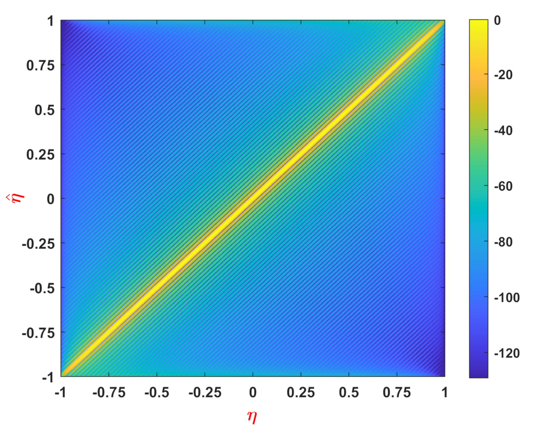
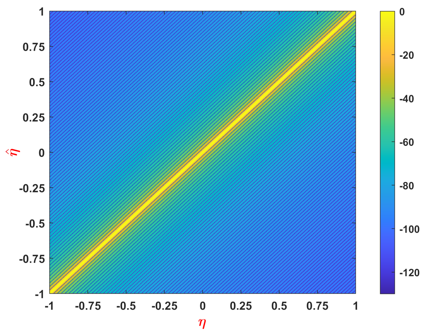
In Figure 2 and Figure 3 the actual kernel of $A_1{A}_1^{†}$ (i.e., the ${\overline{H}}_{11}(\eta ,\widehat{\eta })$ function) and the approximation of such kernel provided by (27) are sketched.

As it can be seen from the figures, the sinc-squared kernel represents a very good approximation of the actual kernel of $A_1{A}_1^{†}$ at the center of the plot, instead, at the edges (for $\widehat{\eta }$ approaching to 1 and $-1$) the approximation is a little bit less accurate.

Under the approximation (23), the eigenvalues of $A_1{A}_1^{†}$ can be analytically evaluated. Indeed, according to [38], the eigenvalues of an operator with a sinc-squared kernel are given by the following equation

$${\lambda }_m\left(A_1{A}_1^{†}\right)=\left\{\begin{array}{cc}{\displaystyle \frac{4\pi a}{\beta {(a^2+z_1^2)}^{1/2}}}\left(1-{\displaystyle \frac{m}{M_1}}\right)& form\le M_1\\ 0& form>M_1\end{array}\right.$$

(29)

where

$$M_1=\left[\frac{4}{\pi }\beta a\eta (X_1,z_1)\right]$$

(30)

with $\left[·\right]$ denoting the nearest integer.

Accordingly, the singular values of the operator $A_1$ are given by

$${\sigma }_m\left(A_1\right)=\left\{\begin{array}{cc}\sqrt{{\displaystyle \frac{4\pi a}{\beta {(a^2+z_1^2)}^{1/2}}}}\sqrt{1-{\displaystyle \frac{m}{M_1}}}& form\le M_1\\ 0& form>M_1\end{array}\right.$$

(31)

From Equation (31), it is evident that the integer $M_1$ provides the number of relevant singular values of the lifting operator in the case of a single observation line in near zone.

If the function $F(x^{\prime },x^{\prime \prime })$ was a generic function of the space $L_2(SD\times SD)$, such a number would be exactly equal to the dimension of space. Since in our problem the square magnitude of the radiated field is given by $|E_1{|}^2=A_{1}F$ with $F(x^{{}^{\prime }},x^{{}^{″}})=J\left(x^{{}^{\prime }}\right)J^{\ast }\left(x^{{}^{″}}\right)$, the scalar $M_1$ represents an upper bound to the dimension of data space.

4. Dimension of Data Space for Multiple Scanning Lines

In this section, the question of providing the dimension of data space in the case of P observation lines in near non-reactive zone is tackled. In such case the square amplitude distributions $|E_1{|}^2$, ... , $|E_P{|}^2$ supported respectively on the sets $O{D}_1$, ... , $O{D}_P$ are related to the current distribution J by the quadratic model

$$\begin{array}{c}|E_1{|}^2=|T_1{J|}^2,\dots ,|E_P{|}^2={\left|T_{P}J\right|}^2\end{array}$$

(32)

With the aim to evaluate the dimension of data space, at first, a linear operator representing the square amplitude distributions $|E_1{|}^2$, ... , $|E_P{|}^2$ is defined. After, a closed-form approximation of the singular values of such an operator is derived. Finally, a good upper bound to the dimension of data space is estimated by counting the number relevant singular values.

To obtain a linear representation of the phaseless data, also in this case the lifting technique is exploited. Hence, by considering as unknown the function $F(x^{{}^{\prime }},x^{{}^{″}})=J\left(x^{{}^{\prime }}\right)J^{\ast }\left(x^{{}^{″}}\right)$, the lifting operator

$$A:F(x^{{}^{\prime }},x^{{}^{″}})\in L_2(SD\times SD)⟶\left\{\right|E_1\left(x\right){|}^2,\dots ,|E_P\left(x\right){|}^2\}\in L_2^{+}\left(O{D}_1\right)\times \dots \times L_2^{+}\left(O{D}_P\right)$$

(33)

is introduced. The latter can be expressed as below

$$A=\left[\begin{array}{c}{A}_1\\ :\\ A_P\end{array}\right]$$

(34)

where $\forall i\in \{1,\dots ,P\}$

$$A_{i}F={\int }_{-a}^{+a}{\int }_{-a}^{+a}{g}_i(x,x^{{}^{\prime }})g_i^{\ast }(x,x^{{}^{″}})F(x^{{}^{\prime }},x^{{}^{″}})d{x}^{{}^{\prime }}d{x}^{{}^{″}}$$

(35)

Now, the quadratic model (32) can be recast as the following linear model

$$|E_1{|}^2=A_{1}F,\dots ,{\left|E_P\right|}^2=A_{P}F$$

(36)

By virtue of (34) and (35), the adjoint operator $A^{†}$ can be expressed as

$$A^{†}=\left[A_1^{†}\dots A_P^{†}\right]$$

(37)

where $\forall i=\{1,\dots ,P\}$

$$A_i^{†}|E_i{|}^2={\int }_{-X_i}^{+X_i}{g}_i^{\ast }(x,x^{{}^{\prime }})g_i(x,x^{{}^{″}}){\left|E_i\left(x\right)\right|}^{2}dx$$

(38)

Since the singular values of the lifting operator A are the square root of the eigenvalues of $A{A}^{†}$, the need of studying the operator $A{A}^{†}$ arises. The latter is given by

$$A{A}^{†}=\left[\begin{array}{c}{A}_1\\ :\\ A_P\end{array}\right]\left[A_1^{†}\dots A_P^{†}\right]=\left[\begin{array}{c}{A}_1{A}_1^{†}\cdots A_1{A}_P^{†}\\ ⋮\ddots ⋮\\ A_P{A}_1^{†}\cdots A_P{A}_P^{†}\end{array}\right]$$

(39)

where $\forall i,j\in \{1,\dots ,P\}$

$$A_i{A}_j^{†}|E_j{|}^2={\int }_{-X_j}^{+X_j}{H}_{ij}(x,\widehat{x}){\left|E_j\left(\widehat{x}\right)\right|}^{2}d\widehat{x}$$

(40)

with

$$H_{ij}(x,\widehat{x})={\left|{\int }_{-a}^a{g}_i(x,x^{\prime })g_j^{\ast }(\widehat{x},x^{\prime })d{x}^{\prime }\right|}^2={\left|z_i{z}_j{\int }_{-a}^{+a}{\displaystyle \frac{e^{-j\beta [R_i(x^{{}^{\prime }},x)-R_j(x^{{}^{\prime }},\widehat{x})]}}{R_i^{3/2}(x^{{}^{\prime }},x)R_j^{3/2}(x^{{}^{\prime }},\widehat{x})}}d{x}^{\prime }\right|}^2$$

(41)

The previous integral can be recast in the following form

$$H_{ij}(x,\widehat{x})={\left|z_i{z}_j{\int }_{-a}^{+a}{f}_{ij}(x^{{}^{\prime }},x,\widehat{x})e^{-j\beta a{\varphi }_{ij}(x^{{}^{\prime }},x,\widehat{x})}d{x}^{\prime }\right|}^2$$

(42)

where

• $f_{ij}(x^{{}^{\prime }},x,\widehat{x})=R_i^{-3/2}(x^{{}^{\prime }},x)R_j^{-3/2}(x^{{}^{\prime }},\widehat{x})$
• ${\varphi }_{ij}(x^{{}^{\prime }},x,\widehat{x})=\frac{1}{a}[R_i(x^{{}^{\prime }},x)-R_j(x^{{}^{\prime }},\widehat{x})]$

At this juncture, in order to provide an explicit expression of $H_{ij}$, let us distinguish the cases $i=j$, and $i\ne j$.

4.1. Kernel Evaluation of the Main Diagonal Terms of $A{A}^{†}$

If $i=j$, from the comparison between (41) and (5), it follows that

$$H_{ii}(x,\widehat{x})={\left|K_{ii}(x,\widehat{x})\right|}^2$$

(43)

Since the kernel $H_{ii}$ is not of convolution type, an analytical study of its eigenvalues may be difficult. To recast it like a convolution kernel, let us pass from the variables $(x,\widehat{x})$ to the variables $\eta =\eta (x,z_i)$$\widehat{\eta }=\eta (\widehat{x},z_i)$. By doing this, it results that $A_i{A}_i^{†}$ can be expressed as

$$A_i{A}_i^{†}|E_i{|}^2={\int }_{\eta (-X_i,z_i)}^{\eta (X_i,z_i)}{\overline{H}}_{ii}(\eta ,\widehat{\eta }){\left|E_i\left(\widehat{\eta }\right)\right|}^{2}d\widehat{\eta }$$

(44)

where

$${\overline{H}}_{ii}(\eta ,\widehat{\eta })=\frac{dx}{d\widehat{\eta }}|K_{ii}(\eta ,\widehat{\eta }){|}^2={\displaystyle \frac{1}{\frac{dx}{d\widehat{\eta }}}}{\left|{\overline{K}}_{ii}(\eta ,\widehat{\eta })\right|}^2$$

(45)

Now, taking into account for (11), the following expression of ${\overline{H}}_{ii}$ comes out

$${\overline{H}}_{ii}(\eta ,\widehat{\eta })\approx {\displaystyle \frac{z_i^4}{{\left(\beta a\right)}^2}}{\displaystyle \frac{dx}{d\widehat{\eta }}}·{\left|\frac{f_{ii}(a,\eta ,\widehat{\eta })}{{\varphi }_{ii}^{\prime }(a,\eta ,\widehat{\eta })}{e}^{j\beta a(\eta -\widehat{\eta })}-\frac{f_{ii}(-a,\eta ,\widehat{\eta })}{{\varphi }_{ii}^{\prime }(-a,\eta ,\widehat{\eta })}{e}^{-j\beta a(\eta -\widehat{\eta })}\right|}^2$$

(46)

As shown in Appendix A, the terms $f_{ii}(-a,\eta ,\widehat{\eta })/{\varphi }_{ii}^{\prime }(-a,\eta ,\widehat{\eta })$ and $f_{ii}(a,\eta ,\widehat{\eta })/{\varphi }_{ii}^{\prime }(a,\eta ,\widehat{\eta })$ can be approximated as

$${\displaystyle \frac{f_{ii}(a,\eta ,\widehat{\eta })}{{\varphi }_{ii}^{\prime }(a,\eta ,\widehat{\eta })}}\approx {\displaystyle \frac{f_{ii}(-a,\eta ,\widehat{\eta })}{{\varphi }_{ii}^{\prime }(-a,\eta ,\widehat{\eta })}}\approx -{\displaystyle \frac{a}{z_i^2{[a^2+z_i^2]}^{1/4}}}{\displaystyle \frac{1}{(\eta -\widehat{\eta }){\left(\frac{dx}{d\widehat{\eta }}\right)}^{1/2}}}$$

(47)

Accordingly, $\forall i=\{1,\dots ,P\}$ the kernel of $A_i{A}_i^{†}$ can be rewrite as below

$${\overline{H}}_{ii}(\eta ,\widehat{\eta })\approx {\displaystyle \frac{4a^2}{\sqrt{a^2+z_i^2}}}sin{c}^2\left(\beta a(\eta -\widehat{\eta })\right)$$

(48)

4.2. Kernel Evaluation of the Off-Diagonal Terms of $A{A}^{†}$

If $i\ne j$ and $\beta a>>1$ then the kernel $H_{ij}$ can be still evaluated by an asymptotic technique but, in such case, the phase function contains also a stationary point which is represented by the solution $x_s$ of the equation

$${\displaystyle \frac{\partial }{\partial x^{\prime }}}{\varphi }_{ij}(x^{\prime },x,\widehat{x})=0$$

(49)

with respect to the variable $x^{\prime }$.

For such reason, the asymptotic evaluation of $H_{ij}$ contains not only the contributions due to the endpoints $x^{\prime }=a$, $x^{\prime }=-a$, but also the contribution of the stationary point $x^{\prime }=x_s$; accordingly, $H_{ij}$ is given by

$$H_{ij}(x,\widehat{x})\approx \left|z_i{z}_j\sqrt{{\displaystyle \frac{2\pi }{\beta a}}}{\displaystyle \frac{f(x_s,x,\widehat{x})}{\sqrt{{\varphi }_{ij}^{\prime \prime }(x_s,x,\widehat{x})}}}{e}^{-j\beta a{\varphi }_{ij}(x_s,x,\widehat{x})}{e}^{j\frac{\pi }{4}sign\left({\varphi }_{ij}^{{}^{\prime \prime }}(x_s,x,\widehat{x})\right)}+\right.$$

$${\left.-{\displaystyle \frac{z_i{z}_j}{j\beta a}}\left(\frac{f_{ij}(a,x,\widehat{x})}{{\varphi }_{ij}^{\prime }(a,x,\widehat{x})}{e}^{-j\beta a{\varphi }_{ij}(a,x,\widehat{x})}-\frac{f_{ij}(-a,x,\widehat{x})}{{\varphi }_{ij}^{\prime }(-a,x,\widehat{x})}{e}^{-j\beta a{\varphi }_{ij}(-a,x,\widehat{x})}\right)\right|}^2$$

(50)

By passing from the variables $(x,\widehat{x})$ to the variables $\eta =\eta (x,z_i)$$\widehat{\eta }=\eta (\widehat{x},z_j)$, the kernel of $A_i{A}_j^{†}$ can be expressed as

$$H_{ij}(\eta ,\widehat{\eta })\approx {\displaystyle \frac{dx}{d\widehat{\eta }}}\left|z_i{z}_j\sqrt{{\displaystyle \frac{2\pi }{\beta a}}}{\displaystyle \frac{f(x_s,\eta ,\widehat{\eta })}{\sqrt{{\varphi }_{ij}^{\prime \prime }(x_s,\eta ,\widehat{\eta })}}}{e}^{-j\beta a{\varphi }_{ij}(x_s,\eta ,\widehat{\eta })}{e}^{j\frac{\pi }{4}sign\left({\varphi }_{ij}^{{}^{\prime \prime }}(x_s,\eta ,\widehat{\eta })\right)}+\right.$$

$${\left.-{\displaystyle \frac{z_i{z}_j}{j\beta a}}\left(\frac{f_{ij}(a,\eta ,\widehat{\eta })}{{\varphi }_{ij}^{\prime }(a,\eta ,\widehat{\eta })}{e}^{-j\beta a{\varphi }_{ij}(a,\eta ,\widehat{\eta })}-\frac{f_{ij}(-a,\eta ,\widehat{\eta })}{{\varphi }_{ij}^{\prime }(-a,\eta ,\widehat{\eta })}{e}^{-j\beta a{\varphi }_{ij}(-a,\eta ,\widehat{\eta })}\right)\right|}^2$$

(51)

Despite Equation (51) provides a closed-form expression of the kernel of $A_i{A}_j^{†}$, a study of such an operator from an analytical point of view is difficult to perform. However, as it will be seen in next sections, some useful considerations can be done to understand the eigenvalues behavior of the operator $A{A}^{†}$.

4.3. The Role of the Distance between the Scanning Lines

In order to predict the eigenvalues of $A{A}^{†}$, the role played by the distance between the i-th and j-th scanning line must be analyzed. From (41), it is evident that if the distance $|z_i-z_j|$ is small then the operator $A_i{A}_j$ is very similar to the operators $A_i{A}_i^{†}$ and $A_j{A}_j^{†}$ which, in turn, are similar to each other. Hence, if $|z_i-z_j|$ is small $\forall i,j\in \{1,2,\dots ,P\}:i\ne j$ then all the operators composing $A{A}^{†}$ are similar and the number of relevant eigenvalues of $A{A}^{†}$ is essentially equal to the case of a single observation line.

On the contrary, when the distance $|z_i-z_j|$ increases, the operator $A_i{A}_j^{†}$ starts to differ from $A_i{A}_i^{†}$ and $A_j{A}_j^{†}$ and such difference becomes more and more evident as such distance raises. In particular, it happens that when the distance between the i-th and the j-th scanning line increases, the norm of the off-diagonal operators $A_i{A}_j^{†}$ strongly decreases. Accordingly, it will exist a minimum value of the distance $|z_i-z_j|$ for which the norm of $A_i{A}_j^{†}$ is negligible with respect to $A_i{A}_i^{†}$ and $A_j{A}_j^{†}$.

To quantify the value of such distance, let us introduce the auxiliary operator $T_z$ linking the magnetic current density $J\left(x^{\prime }\right)\in L_2\left([-a,a]\right)$ to $E(x_o,z)\in L_2\left([z_{min},z_{max}]\right)$, i.e., the $x$—component of the electric field evaluated along the axis $x=x_o$ for $z_{min}\le z\le z_{max}$.

The introduction of such an operator allows to consider the point spread function in the observation domain associated to it which represents the most focusing field with the maximum in the point $z=z_o$ that the source is able to radiate along the axis $x=x_o$.

From the mathematical point of view, the point spread function in the observation domain is the impulsive response of the system made up by the cascade of the regularized inverse operator $T_z^{-1}$ and the forward one, hence, it is defined as

$$PSF(z,z_o)=T_z{T}_z^{-1}\delta (z-z_o)$$

(52)

where $\delta (z-z_o)$ is the impulse function.

In our discussion, the point spread function in the observation domain is used to estimate the optimal points where the radiated electric field $E(x_o,z)$ must be sampled not to lose relevant information in the discretization process. Next, from the knowledge of the optimal sampling points in the case of data in amplitude and phase, an useful criterion for the spacing between adjacent observation domains in the case of phaseless measurements is derived.

To do this, let us derive an explicit expression of the point spread function. Since the inverse operator $T_z^{-1}$ can be approximated by a weighted adjoint operator $T_{zw}^{†}$ [39], it results that

$$PSF(z,z_o)\approx T_z{T}_{zw}^{†}\delta (z-z_o)$$

(53)

A closed-form expression of the operator $T_z{T}_{zw}^{†}$ is provided in [40]. Hence, on the basis of such result, an approximation of the point spread function in the observation domain is given by

$$PSF(z,z_o)\approx e^{jW\left(\nu \left(z_o\right)-\nu \left(z\right)\right)}sinc\left(W\left(\zeta \left(z\right)-\zeta \left(z_o\right)\right)\right)$$

(54)

with

$$W=\left\{\begin{array}{c}\beta afor|x_o|\ge a\hfill \\ \beta {\displaystyle \frac{a+|x_o|}{2}}for\left|x_o\right|\le a\hfill \end{array}\right.$$

(55)

$$\begin{array}{c}\nu \left(z\right)\hfill \\ \zeta \left(z\right)\hfill \end{array}=\left\{\begin{array}{c}{\displaystyle \frac{\sqrt{\left(\right|x_o{|+a)}^2+z^2}\pm \sqrt{\left(\right|x_o{|-a)}^2+z^2}}{2a}}for\left|x_o\right|>a\hfill \\ {\displaystyle \frac{\sqrt{\left(\right|x_o{|+a)}^2+z^2}\pm \left|z\right|}{a+|x_o|}}for\left|x_o\right|\le a\hfill \end{array}\right.$$

(56)

where the signum $(+)$ holds for $\nu$ while $(-)$ holds for $\zeta$, respectively.

As shown in [41], the zeros of the point spread function in the observation domain represent the optimal sampling points of the radiated field; for such reason, $E(x_o,z)$ must be sampled at the points $\left\{z_{i+1}\right\}$ satisfying the equation $W[\zeta \left(z_{i+1}\right)-\zeta \left(z_i\right)]=i\pi$.

However, our main aim is that of finding a sampling strategy of $|E(x_o,z){|}^2$. This can be easily done by remembering that the bandwidth of the square magnitude of a function is twice the one of the corresponding function. For such reason, the optimal sampling points of $|E(x_o,z){|}^2$ are given by

$$2W[\zeta \left(z_{i+1}\right)-\zeta \left(z_i\right)]=i\pi$$

(57)

Equation (57) provides the minimum distance for which two samples of $|E(x_o,z){|}^2$ collected at different values of z are independent to each other. Hence, it could give a guideline in the choice of the spacing $\Delta z_i=z_{i+1}-z_i$ between two adjacent scanning lines in the case of phaseless measurements.

However, from Equation (57), it is evident that the distance between the samples of $|E(x_o,z){|}^2$ depends also on $x_o$ or, in other words, the value of $z_{i+1}$ obtained by solving (57) is a function of $x_o$ with $x_o\in [-X_i,X_i]$. For such reason, to ensure that the data collected on the $(i+1)$-th observation domain are independent by those collected on the $i$-th observation domain, the value of $z_{i+1}$ must be chosen at least equal to the maximum value of the function $z_{i+1}\left(x_o\right)$ derived by inverting (57). Hence, the spacing $\Delta z_i=z_{i+1}-z_i$ between two adjacent scanning line is dictated by the maximum value of $z_{i+1}\left(x_o\right)$ which is achieved for $x_o=0$ or $x_o=X_i$.

From the previous discussion, it follows that a reasonable criterion for the choice of $z_{i+1}$ is the following

$$z_{i+1}\ge max\{z_{i+1}\left(0\right),z_{i+1}\left(X_i\right)\}$$

(58)

where $z_{i+1}\left(0\right)$ and $z_{i+1}\left(X_i\right)$ are the solutions of the equations

$$\sqrt{a^2+z_{i+1}^2\left(0\right)}-\left|z_{i+1}\left(0\right)\right|=i{\displaystyle \frac{\pi }{\beta }}+\sqrt{a^2+z_i^2}-\left|z_i\right|$$

(59)

$$\sqrt{{(X_i+a)}^2+z_{i+1}^2\left(X_i\right)}-\sqrt{{(X_i-a)}^2+z_{i+1}^2\left(X_i\right)}=i{\displaystyle \frac{\pi }{\beta }}+\sqrt{{(X_i+a)}^2+z_i^2}-\sqrt{{(X_i-a)}^2+z_i^2}$$

(60)

Hence, if the distance between two adjacent scanning lines is chosen according to the criterion (58), the norm of all the off-diagonal operators $A_i{A}_j$ is negligible with respect to the norm of the operator on the main diagonal. In such condition, the operator $A{A}^{†}$ can be expressed as below

$$A{A}^{†}\approx \left[\begin{array}{c}\begin{array}{c}{A}_1{A}_1^{†}\\ 0\\ ⋮\\ 0\end{array}\begin{array}{c}0\\ A_2{A}_2^{†}\\ ⋮\\ 0\end{array}\begin{array}{c}\cdots \\ \cdots \\ \ddots \\ \cdots \end{array}\begin{array}{c}0\\ 0\\ ⋮\\ A_P{A}_P^{†}\end{array}\end{array}\right]$$

(61)

4.4. The Dimension of Data Space

Under the approximations (61) and (48) , the eigenvalues of $A{A}^{†}$ can be analytically computed; in particular, they are given by the union of the eigenvalues of the operators on the main diagonal, i.e.,

$$\left\{{\lambda }_m\left(A{A}^{†}\right)\right\} \approx \left\{{\lambda }_m\left(A_1{A}_1^{†}\right)\right\}\cup \dots \cup \left\{{\lambda }_m\left(A_P{A}_P^{†}\right)\right\}$$

(62)

where $\forall i\in \{1,\dots ,P\}$

$${\lambda }_m\left(A_i{A}_i^{†}\right)= \left\{\begin{array}{cc}{\displaystyle \frac{4\pi a}{\beta {(a^2+z_i^2)}^{1/2}}}\left(1-{\displaystyle \frac{m}{M_i}}\right)& form\le M_i\\ 0& form>M_i\end{array}\right.$$

(63)

with $M_i=\left[\frac{4}{\pi }\beta a\eta (X_i,z_i)\right]$.

Accordingly, the singular values of the lifting operator A are given by

$$\left\{{\sigma }_m\left(A\right)\right\}\approx \left\{{\sigma }_m\left(A_1\right)\right\}\cup \dots \cup \left\{{\sigma }_m\left(A_P\right)\right\}$$

(64)

where $\forall i\in \{1,\dots ,P\}$

$${\sigma }_m\left(A_i\right)=\sqrt{{\lambda }_m\left(A_i{A}_i^{†}\right)}=\left\{\begin{array}{cc}\sqrt{{\displaystyle \frac{4\pi a}{\beta {(a^2+z_i^2)}^{1/2}}}}\sqrt{1-{\displaystyle \frac{m}{M_i}}}& form\le M_i\\ 0& form>M_i\end{array}\right.$$

(65)

From the previous analysis, it comes out that the total number of relevant singular values of the lifting operator A can be expressed as

$$M\approx \sum _{i=1}^P{M}_i=\sum _{i=1}^P\left[{\displaystyle \frac{4}{\pi }}\beta a\eta (X_i,z_i)\right]$$

(66)

If the extension of the observation lines $X_1,\dots ,X_P$ are such that $\eta (X_1,z_1)=\dots =\eta (X_P,z_P)={\eta }_{max}$, the previous equation particularizes as below

$$M\approx \left[{\displaystyle \frac{4P}{\pi }}\beta a{\eta }_{max}\right]$$

(67)

The scalar M represents the desired upper bound to the dimension of data space in the case of P observation lines.

It is worth highlighting that Equation (67) is very similar to Equation (46) shown in [35], i.e., $M\approx \frac{4P}{\pi }\beta a{u}_{max}$. The latter represents the number of relevant singular values of the lifting operator when the observation domain is an ensemble of P observation arcs in Fresnel zone subtending an angular sector $[-{\theta }_{max},{\theta }_{max}]$. As can be seen, the relevant difference between Equation (67) of this article and Equation (46) in [35] is that ${\eta }_{max}$ is replaced by $sin{\theta }_{max}$. This is perfectly consistent with the fact that the variable $\eta$ in Fresnel zone can be approximated by $sin\theta$.

5. Numerical Simulations

In this section, some numerical simulations that confirm the analytical results of Section 3 and Section 4 are shown.

The numerical tests are performed by considering a source with a semi-length $a=20\lambda$ whose square magnitude of the radiated field is observed on 1 or 2 truncated observation lines in near zone.

5.1. Numerical Simulations for a Single Observation Line

In this section, numerical simulations for the case of 1 observation line are provided.

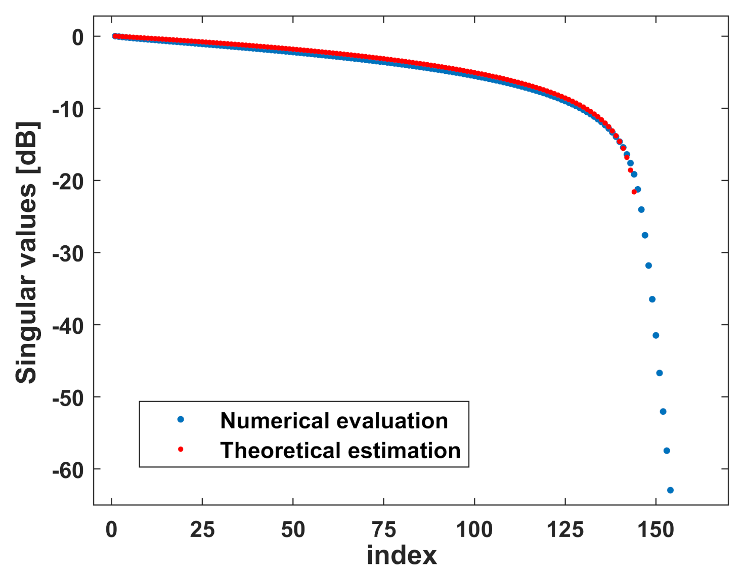
As first example, an observation domain with $z_1=5\lambda$, $X_1=20.75\lambda$$(\eta (X_1,z_1)=0.9)$ is considered.

In order to check the theoretical result provided by (30), in Figure 4 the singular values of the lifting operator $A_1$ and their analytical estimation are compared.

As can be seen from Figure 4, the two diagrams exactly overlap until to the index $M_1=144$ which represents an upper bound to the dimension of data space. This means that the number of relevant singular values is exactly predicted by (30) whereas their value is well estimated by (31).

A second test has been performed for a configuration with $z_1=5\lambda$, $X_1=37\lambda$$(\eta (X_1,z_1)=0.99)$. Hence, in such case, the observation domain has been significantly extended along the x-axis.

With reference to such a configuration, in Figure 5 the singular values of the lifting operator and their analytical estimation provided by (31) are sketched.

Sinc in this case the approximation of the kernel of $A_1{A}_1^{†}$ with a sinc square function is a little bit less accurate, also the approximation of the singular values provided by (31) is a little bit less accurate than the previous test case.

As concerns the number of relevant singular values, it is exactly equal for both the diagrams and correctly predicted by the Equation (30) which returns $M_1=158$.

5.2. Numerical Results for Two Observation Lines

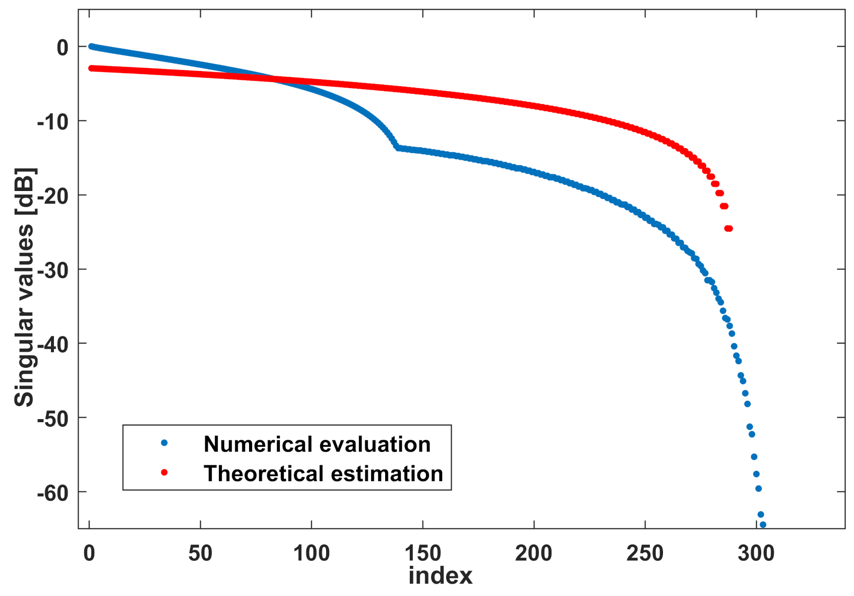
In this section, with reference to the case of 2 observation domains, some key numerical experiments are shown. In all the test cases, the semi-extensions of the observation domains $X_1$ and $X_2$ are chosen in such a way that $\eta (X_1,z_1)=\eta (X_2,z_2)={\eta }_{max}$.

As a first test case, a configuration with $z_1=5\lambda$, $z_2=5.25\lambda$ is considered. The extension of the observation domains is such that $\eta$ changes on the set $[-0.9,0.9]$; hence, it results that $X_1=20.75\lambda$, $X_2=21.01\lambda$.

Since the distance $z_1$ and $z_2$ are very similar, the operators $A_1{A}_1^{†}$, $A_1{A}_2^{†}$, $A_2{A}_1^{†}$, $A_2{A}_2^{†}$ does not differ significantly each other. Hence, also their eigenvalues (that are sketched in Figure 6) exhibit the same decay. Accordingly, in such case, the second scanning line does not increase significantly the number of significant singular values, and the dimension of data space remains essentially equal to the case of 1 scanning line. This fact is confirmed also by Figure 7 in which the singular values of $A_1$ are sketched in blue.

In the second test case, a configuration with $z_1=5\lambda$, $z_2=5.67\lambda$ is analyzed. Also in this case, the extension of the observation lines is such that $\eta \in [-0.9,0.9]$; hence, $X_1=20.75\lambda$ and $X_2=21.47\lambda$.

The main difference between this configuration and that considered before is the choice of the distance $z_2$ which, in this experiment, has been increased and chosen according to the criterion (58). As stated in Section 4, when the distance $|z_2-z_1|$ increases, the norm of the off-diagonal terms $A_1{A}_2^{†}$ and $A_2{A}_1^{†}$ decreases with respect to the norm of $A_1{A}_1^{†}$ and $A_2{A}_2^{†}$. For each $i,j\in \{1,2\}$, the norm of the self-adjoint operator $A_i{A}_j^{†}$ can be evaluated through the equation

$$\left|\right|A_i{A}_j^{†}\left|\right|=\sqrt{{\sum }_{m=1}^{+\infty }{\lambda }_m^2\left(A_i{A}_j^{†}\right)}$$

(68)

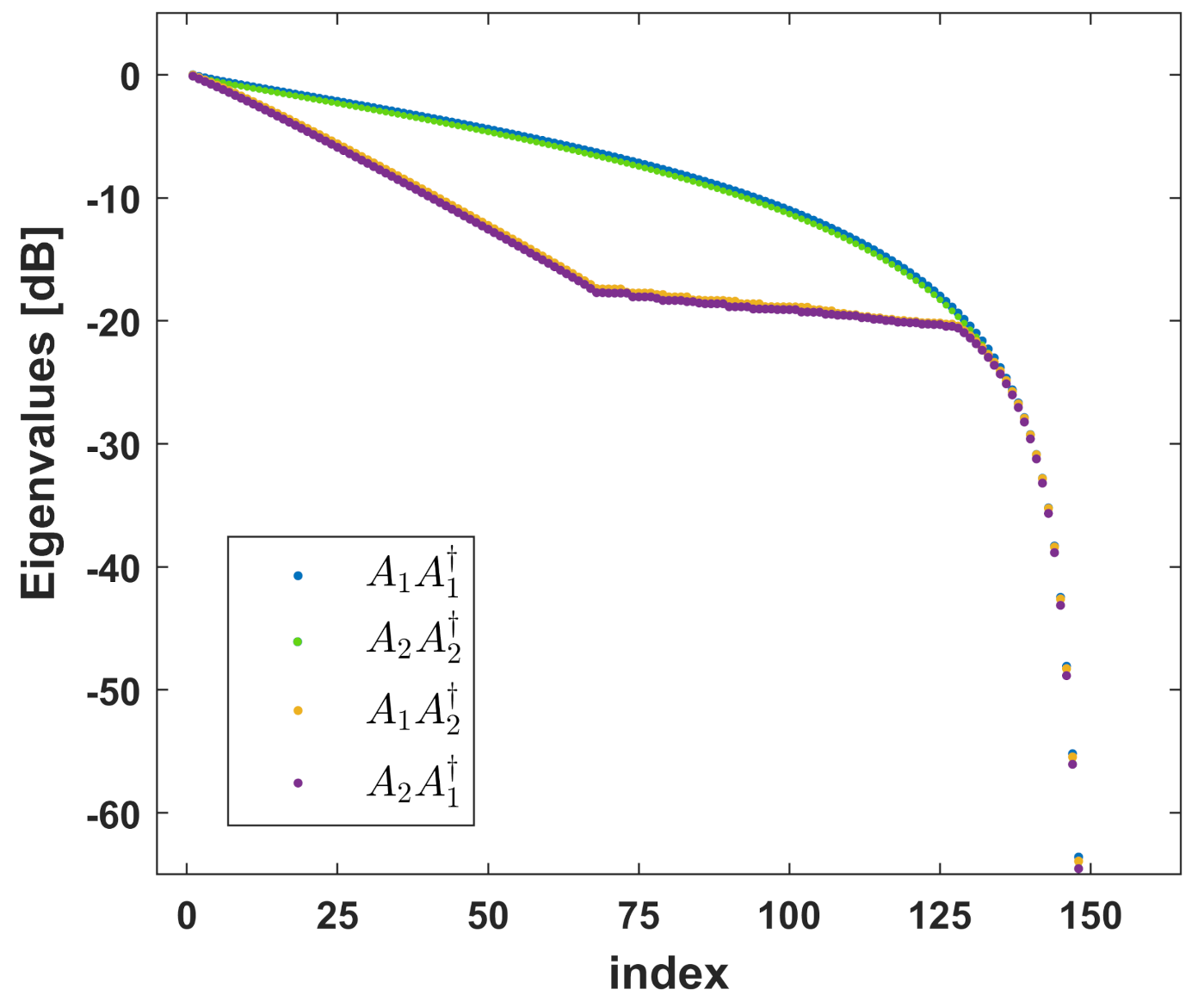
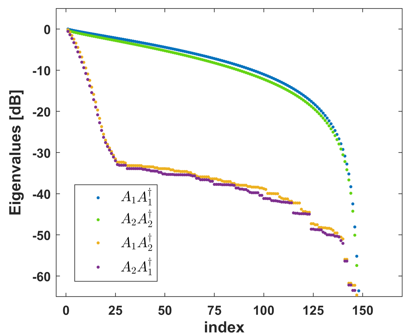
Hence, the relation between the norm of $A_1{A}_1^{†}$, $A_1{A}_2^{†}$$A_2{A}_1^{†}$$A_2{A}_2^{†}$ can be understood by a simple plot of their eigenvalues which is sketched in Figure 8.

As can be seen from Figure 8, the eigenvalues of the off-diagonal terms ($A_1{A}_2^{†}$, $A_2{A}_1^{†}$) decay quite faster than the eigenvalues of the terms on the main diagonal ($A_1{A}_1^{†}$, $A_2{A}_2^{†}$). Therefore, $\left|\right|A_1{A}_1^{†}\left|\right|$ and $\left|\right|A_2{A}_2^{†}\left|\right|$ are greater than $\left|\right|A_1{A}_2^{†}\left|\right|$ and $\left|\right|A_2{A}_1^{†}\left|\right|$. Accordingly, at least the number of significant singular values of A can by approximated by (66).

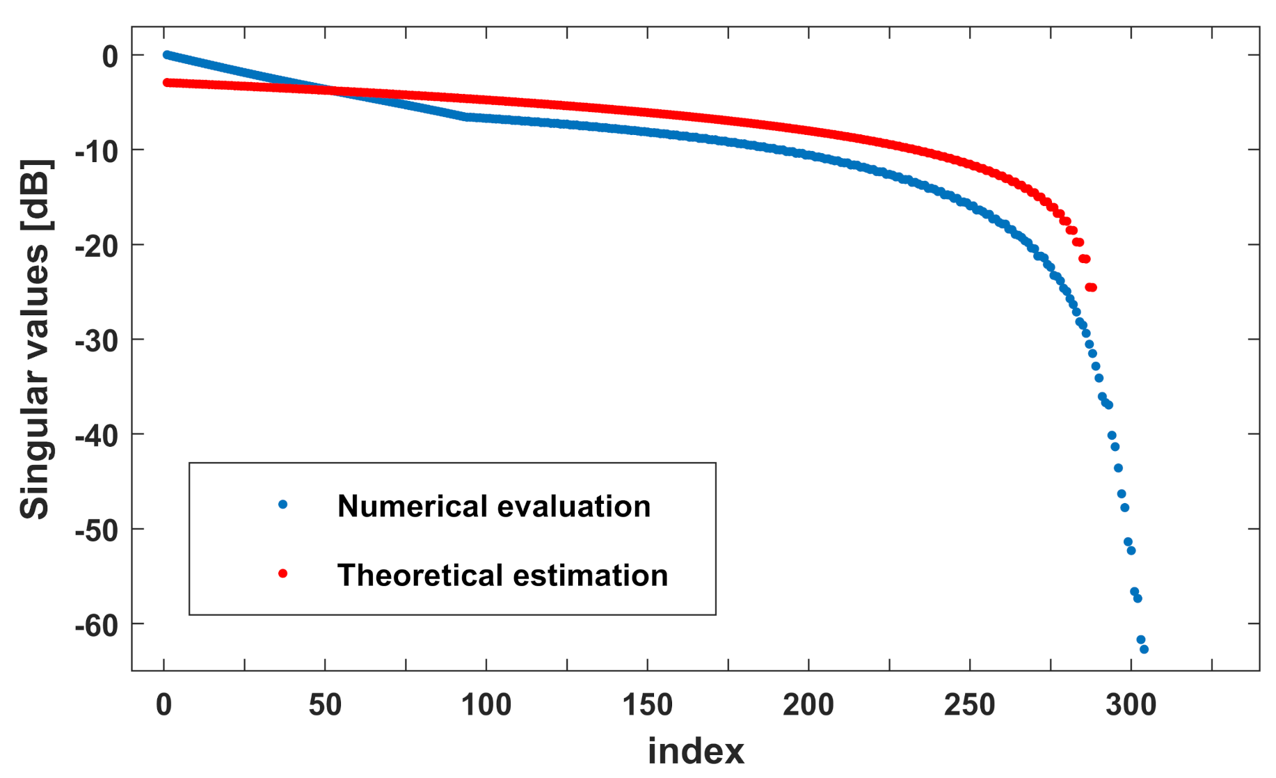
In Figure 9, the singular values of A numerically computed are compared with their analytical estimation provided by (65).

As shown by such figure, the estimation of the number of relevant singular values M is quite good and equal to 288 as predicted by (66); however, the approximation of the singular values is not so accurate. This happens since the norm of the off-diagonal terms of $A{A}^{†}$ (despite negligible with respect to the terms on the main diagonal) does not approach to zero. For such reason, there is still a small effect brought by the off diagonal terms of $A{A}^{†}$ on its eigenvalues, and consequently, on the singular values of A.

Hence, it is possible to conclude that the choice of the minimum distance satisfying the criterion (58) is sufficient to ensure that the data collected on the second scanning are independent by those collected on the first scanning but it does not allow to reach the minimum dynamics of the singular values of the lifting operator.

A third test case concerns the configuration $z_1=5\lambda$, $z_2=7.5\lambda$, $X_1=20.75\lambda$ ($\eta (X_1,z_1)=0.9$), $X_2=23.75\lambda$ ($\eta (X_1,z_1)=0.9$). Hence, the distance $|z_2-z_1|$ has been further increased with respect to the previous one. In this test case, the eigenvalues of $A_1{A}_2^{†}$ and $A_2{A}_1^{†}$ decay faster then the previous case (see Figure 10); hence, the ratio between the norm of the off-diagonal terms and the norm of the main diagonal terms is smaller than the previous case. This imply that the approximation of the singular values provided by (65) is more accurate.

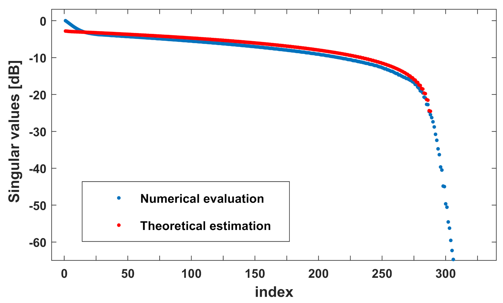
In Figure 11, the singular values of A are compared with their theoretical approximation. From such plot, it is evident that in the considered case our theoretical estimations predict accurately not only the dimension of data space ($M_1=288$) but also their value.

A final test case has been done for the configuration $z_1=5\lambda$, $z_2=7.5\lambda$, $X_1=37.03\lambda$ ($\eta (X_1,z_1)=0.99$), $X_2=50.97\lambda$ ($\eta (X_2,z_2)=0.99$). Hence, with respect to the previous case, the extension of the observation lines has been enlarged while the distance between them is unchanged.

With reference to such a configuration, in Figure 12 the singular values of A numerically computed are compared with the analytical estimation provided by (65). From such plot it is evident that, despite the distance $|z_2-z_1|$ is large enough, the number of relevant singular values is well predicted by (66) but the estimation of the value of the singular values is less accurate than the example in Figure 11. This aspect can be easily understood by remembering that the approximations (47) and (48) work well when the maximum value of $\eta$ and $\widehat{\eta }$ does not approach to 1. In considered example, the maximum value of such variables is equal to $0.99$. For such reason, the approximation of the kernel of $A_1{A}_1^{†}$ and $A_2{A}_2^{†}$ with the correspondent sinc square function is not so accurate and, consequently, the estimation of the singular values provided by (65) does not match perfectly with its numerical evaluation.

6. Conclusions

In this article, the question of evaluating the dimension of data space in the quadratic formulation of phase retrieval problem has been addressed. In particular, a good upper bound to the dimension of the functional space containing all the possible square magnitude of the near-field radiated by a magnetic current strip on one and multiple lines parallel to the source non-reactive zone has been estimated.

Such analysis has been developed in multiple steps. In particular, after having introduced the linear lifting operator representing the phaseless data, the upper bound to the dimension of data space has been defined as the number of relevant singular values of such an operator.

With the aim to estimate the number of relevant singular values of the lifting operator, the kernel of the related eigenvalue problem has been first approximated by asymptotic reasoning, and after, it has been recast as a convolution kernel by exploiting a proper change of variables. Finally, the eigenvalues of such an operator have been analytically computed and, from these, the value and the number of relevant singular values have been derived.

Let us remark that our analytical results on the dimension of data space allow to show how the geometrical parameters of the configuration affect the dimension of data space.

Moreover, before concluding, it is worth noting that the adopted methodology for estimating an upper bound to the dimension of data space is quite general, hence, it can be extended also to other geometries.