Article

Robust Model Predictive Controller Using Recurrent Neural Networks for Input–Output Linear Parameter Varying Systems

1
College of Electrical and Computer Engineering, Tarbiat Modares University, Tehran 14117-13116, Iran
2
College of Engineering, Department of Mechanical Engineering, University of Saskatchewan, Saskatoon, SK S7N 5E5, Canada
*
Author to whom correspondence should be addressed.
Electronics 2021, 10(13), 1557; https://doi.org/10.3390/electronics10131557
Submission received: 2 June 2021 / Revised: 21 June 2021 / Accepted: 22 June 2021 / Published: 28 June 2021
(This article belongs to the Special Issue Control Applications and Learning)

Abstract

:
This paper develops a model predictive controller (MPC) for constrained nonlinear MIMO systems subjected to bounded disturbances. A linear parameter varying (LPV) model assists MPC in dealing with nonlinear dynamics. In this study, the nonlinear process is represented by an LPV using past input–output information (LPV-IO). Two primary objectives of this study are to reduce online computational load compared with the existing literature of MPC with an LPV-IO model and to confirm the robustness of the controller in the presence of disturbance. For the first goal, a recurrent neural network (RNN) is employed to solve real-time optimization problems with lower online computation. Regarding robustness, a new control law is developed, which comprises a fixed control gain ( K ) and a free perturbation ( C ) . The proposed method enjoys a shrunken conservatism owing to the finding of a larger possible terminal region and using free control moves. The strategy is examined in an alkylation of benzene process and displays outstanding performance in both setpoint tracking and disturbance rejection problems. Moreover, the superiority of RNN over three conventional optimization algorithms is underlined in terms of MSE, the average time for solving the optimization problem, and the value of the cost function.

1. Introduction

Over the past few decades, model predictive controllers (MPCs) have attracted a great deal of attention in industry and academia [1,2,3,4]. This considerable prominence of MPC is rooted in several factors, including simple generalization to a MIMO system, applicability to non-minimum phase and unstable processes, capability to compensate delay, and imposing output/input constraints [1]. While influential theories exist in MPC for linear systems, some systems are nonlinear and operate under large operating conditions, or some external parameters can fundamentally change the process response [5]. Nonlinear MPC (NMPC) has been developed to deal with systems with nonlinear dynamics. A higher level of algorithm complexity and excessive computational load are two main drawbacks of NMPC.
A linear parameter varying (LPV) framework is established in this paper to mitigate these problems by assisting the MPC to model dynamic and static nonlinearities [6,7,8,9]. MPC founded on LPV has aroused enthusiasm among researchers to ensure practical implementation to bridge the gap between linear MPC and NMPC [10,11,12] (less complicated than nonlinear models and more accurate than linear models). With the help of LPV, MPC can be employed for nonlinear and/or time-varying systems [6,13,14,15]. LPV offers MPC a linear model instead of nonlinear models, where the scheduling variable denotes nonlinear dynamic parameters, changing environmental conditions, and operating points. It is also noteworthy that, in an LPV model, current values of scheduling variables can be measured or estimated, but the future values are unknown, so a robust MPC is required, or the future values can be estimated.
Most MPC-LPV literature is centered around the state-space model, while states might not be measurable in many industrial applications. Moreover, using an observer can complicate the design. In Reference [16], MPC-LPV with SS and IO presentations are compared for a control moment gyroscope (CMG). The results showed that the execution time would be reduced when using the IO framework. To this end, MPC is established based on an LPV-IO framework in this paper.
Only a few MPCs have been documented for LPV systems under the I/O formulation, mainly focused on stability, computation, and conservatism [5]. One of the initial research works on MPC with the LPV-IO model can be found at [10], where min-max (worse-case) cost functions are regarded. The cost function includes a stage cost for control performance and a terminal cost to grant stability. The optimization problem of MPC is written in bilinear matrix inequality (BMI), which can be non-convex and challenging. This approach was improved in [17] in order to reduce the complexity level markedly. The authors designed a controller based on a linear matrix inequality (LMI) convex problem, successfully assessed in an ideal continuous stirred tank reactor (CSTR). They also enlarge the terminal region to moderately reduce conservatism. This work employed offline controllers and terminal regions to reduce the online computational burden moderately. However, the controller still suffers from substantial online computational capacity, stemming from solving LMI equations and calculating the Markov coefficient of the LPV system [18]. Above all, it is assumed that the future values of scheduling variables can vary inside a convex polytope. This assumption is less conservative than a frozen or fixed scheduling variable over the prediction horizon while making the optimization problem nonlinear or unreachable [5,17]. The online computational complexity of [17] has been slightly ameliorated in a sequence of quadratic programs. The main drawback of this work is that it lacks a provision for recursive feasibility.
The first novelty of our paper is to make the controller, developed in [10], more computationally efficient. To the best of our knowledge, for the first time, a computationally efficient MPC with an LPV-IO model was presented in this study while keeping the conservatism degree as low as reasonably achievable. A recurrent neural network (RNN) is proposed to deal with the online optimization problem in this paper. Thanks to the global convergence and low computational burden, neural network-based optimizations have been applied to linear, quadratic [19,20], nonlinear programming [21,22], and variational inequality problems [23,24]. The RNN is pointed out to display convincing performance in either MPC or NMPC [25,26,27], in which nonlinear optimization can be converted to quadratic programming. The motive behind selecting RNN is its good adaptability as well as lower complexity, even in real-time nonlinear and large-scale optimization. That is why the studied method was assessed in the alkylation of benzene process, a large-scale nonlinear process with 25 state variables, 5 inputs, and 5 outputs.
The second novelty of this paper is to guarantee the robustness of the system when facing bounded disturbance. The problem of disturbance rejection has not been studied so far for MPC with LPV-IO models. A stabilizing control law based on the input–output measurements is proved to ensure the superior closed-loop performance of the controller in the presence of additive disturbance. The control law includes a fixed control gain ( K ) and a free perturbation ( C ), the former of which is designed offline with the largest possible terminal region to reduce conservatism. The free control moves are determined online to ensure input-state stability in the presence of bounded disturbances. Adding control moves provides a less conservative framework than those studied in [17,18], where only offline control gain is employed.
To sum up, the contributions of this paper are as follows:
  • An RNN-based optimization algorithm is developed to offer global convergence and lower the online computational load.
  • Free control moves are added to the constant control gain to maintain the closed-loop stability when facing bounded disturbances.
  • Concerning previous studies for MPC with LPV, the proposed method inherently enjoys a shrunken conservatism degree as a result of finding the larger possible terminal region, using free control moves, and the global solution of the optimization problem.
The rest of the paper is organized as follows. The standard nonlinear model is reformulated as an LPV-IO model in Section 2. The proposed RMPC-LPV structure is developed in Section 3 and proved to be stable and feasible. The MPC-RNN is presented in Section 4. Next, the state-space equations, inputs, outputs, and critical parameters of the alkylation of benzene process are wholly outlined in Section 5, followed by a collection of simulations to evaluate the proposed control methodology. Key findings are finally summarized in Section 6.

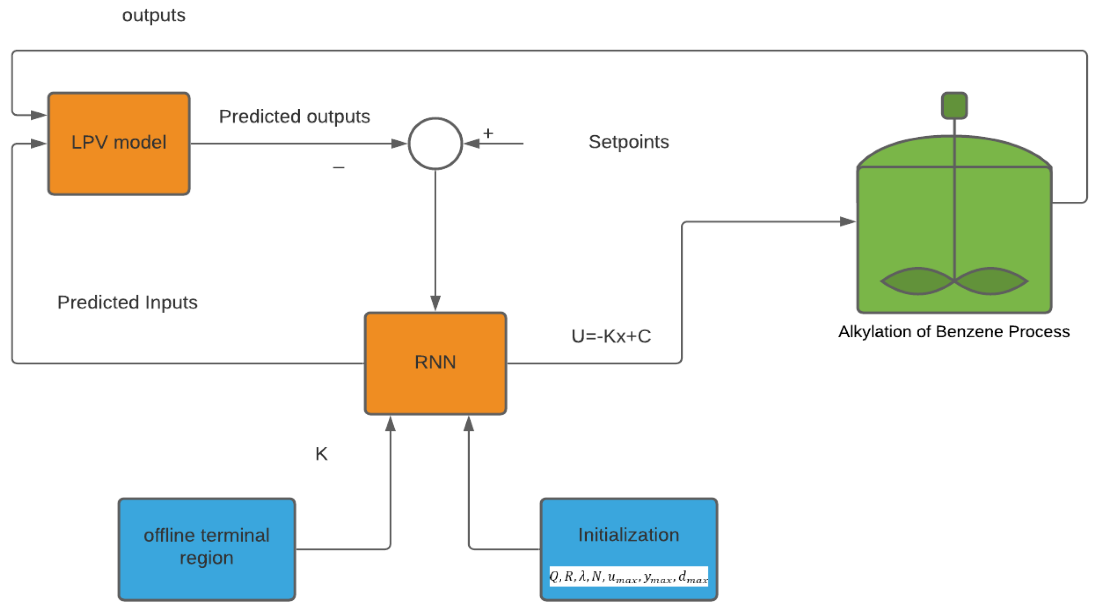
2. Problem Statement

Assume the following discrete-time MIMO linear parameter-varying (LPV) transfer function with constraints:
y ( k ) = ( i = 1 n a A i ( p ( k ) ) q i ) y ( k ) ( j = 1 n b B j ( p ( k ) ) q j ) u ( k ) + d ( p ( k ) )
Subject to the following constraints
u ( k ) U { u n u |   | u ( k ) | u m a x } Δ u ( k ) V { Δ u n u |   | Δ u ( k ) | Δ u m a x } y ( k ) Y { y n y |   | y ( k ) | y m a x }
where y ( k ) are outputs; u ( k ) are inputs; p ( k ) are scheduling variables; q i is backshift operator; n a is the degree of the output polynomial ; n b is the degree of the input polynomial;   n u is the number of input; n y is the number of outputs; and u m a x ,   Δ u m a x , and y m a x are boundaries. The state-space representation of the dynamic model given by Equation (1) is as follows [10]:
x ( k + 1 ) = [ a 1 a n a 1 I n y 0 0 0 0 0 I n y 0 0 0 a n a b 0 + b 1 0             0 0 0 0 0             0 I n u I n u 0 b n b 1 b n b 0 0 0 0 0 0 I n u 0 0 0 0 ] A ( p ( k ) ) x ( k ) + [ b 0 0 0 I n y 0 0 ] B ( p ( k ) ) u ( k ) + d ( k )
where x ( k ) = [ y ( k 1 ) y ( k n a )   u ( k 1 ) u ( k n b ) ] T . For the sake of simplicity, p ( k ) is removed from all coefficients a i and b i . The following assumptions are made:
A1: The parameter-varying matrix is [ A ( k )   B ( k ) ] Ω = C o [ [ A 1   B 1 ] , , [ A m   B m ] ] , where Ω is the polytope,   C o is the convex hull, and [ A i   B i ] are vertices corresponding to scheduling variable p i :
p = C o { p 1 , p m }
A2: The profile of changes in scheduling variables is predetermined from a safety and economic point of view with the following upper and lower bound:
p P { p n p |   | p ( k ) | p m a x }
A3: The disturbance is bounded:
d ( k ) D { d n d |   | d ( k ) | d m a x }  
A4: System 3 is controllable, i.e., the controllability matrix (M) has a full rank:
M = [ B   A B   A 2 B A n 1 B ]  

3. Robust Model Predictive Controller

This paper aims to define a control law that ensures the input-to-state practical stability (ISpS) of the system (1) with constraints (2). The control law is calculated by minimizing the cost function at any time instance k:
V N ( x k , u k , p k ) = k = 0 N 1 [ e ( k + i ) T Q e ( k + i ) + Δ u ( k + i 1 ) T R Δ u ( k + i 1 ) ] + [ x ( k + N ) T Q p x ( k + N ) ] Subject   to   y ( k + j ) = ( i = 1 n a A i q i ) y ( k + j ) ( j = 1 n b B i q i ) u ( k + j ) + d ( k ) ,   j = 1 , 2 , , N 1 u ( k + j ) U Δ u ( k + j ) V y ( k + j ) Y x ( k + N ) X f  
where e = r y , the deviation of output from the reference trajectory, and Δ u is the control increment. Q and R are positive definite state and input weighting matrices in charge of closed-loop achievements, Q p = Q p T > 0 is the terminal penalty matrix designed to ensure stability, and X f is the terminal region. The first and second part of V N are named stage cost ( V s ) and terminal cost ( V T ), respectively. Disturbances are supposed to be fixed over the prediction horizon.
According to [28], a state feedback controller can represent the system’s stability with the LPV-IO form. The control law ( u ( k ) ) is comprised of a fixed state feedback K and a free control move ( c ), in which K is computed offline and c is obtained from the minimization of (8):
u ( k ) = K x ( k ) + c ( k )
The state-feedback gain accounts for maintaining the final state variable x ( k + N ) in the terminal region while meeting constraints and keeping the controller as less conservative as possible. In fact, a constant state feedback controller confirms the stability when there is no disturbance. Otherwise, free control moves (c) will be determined online in a min-max problem to guarantee the ISpS. Thus, a part of the controller will be calculated offline for conditions in which there is not any disturbance, and a part of the controller will be set online to deal with existing disturbances or violation of x ( k + N ) X f .

3.1. Offline Controller

In this section, the stability of the system will be represented when x ( k ) X f through finding control gain K . After calculating the offline controller, a procedure to specify the terminal region is defined.
Theorem 1.
Taking a disturbance-free state-space model of Equation (3), there exists a control law u = K x   that asymptotically stabilizes the system if V T is a positive definite Lyapunov function such that
  • V T ( x ( k + 1 ) ) V T ( x ( k ) ) < 0 for   x X f And   p P .
  • If x ( k ) X f then x ( k + 1 ) X f
  • | u | = | K x | u m a x   f o r     x X f .
Proof. 
Considering V T = x ( k ) T Q p x ( k ) > 0 as the candidate Lyapunov function, the controller u = K x exists, if the equation below satisfies the following:
V T ( x ( k + 1 ) ) V T ( x ( k ) ) < 0 x ( k + 1 ) T Q p x ( k + 1 ) x ( k ) T Q p x ( k ) x ( k ) T Q x ( k ) Δ u ( k ) T R Δ u ( k )
It is assumed that there exists a K such that A B K is stable for all possible pairs of [ A ( k )   B ( k ) ] Ω . By substituting Δ u = K x and x ( k + 1 ) = ( A B K ) x ( k ) , it yields
( ( A B K ) x ( k ) )   T Q p ( ( A B K ) x ( k ) ) x ( k ) T Q p x ( k ) x ( k ) T Q x ( k ) ( K x ( k ) ) T R ( K x ( k ) )
It can be rewritten in a more compact form:
M T Q p M Q p + Q + K T R K 0 M = A B K
Therefore, V T is a Lyapunov function, and the stabilizing state-feedback gain K can be found from (12). After showing the controller’s stability, the terminal region is required to be specified, reducing the conservatism level. The terminal region X f is considered to be an ellipsoidal invariant set:
X f = { x R n | x ( k + N ) T Q p x ( k + N ) < θ }
While X f is intended to be as broad as possible to reduce conservatism, it might lead to extensive control law and violation of input constraints. The maximum value of γ can be derived from an optimization problem such that input limitations are met:
max θ Subject   to x ( k + N ) T Q p x ( k + N ) < θ | K x | u m a x
In Reference [10], it is proved that γ can equivalently be derived from the following optimization problem:
min γ θ θ 2 A T P 1 A T T B T B T T
where A T = [ I n   K   I n K ] T ,   B T = [ x m a x x s   Δ u m a x   x m a x x s   Δ u m a x ] T , and x s is the desired state. In this section, an offline state-feedback controller ( K ) and the corresponding terminal region ( X f ) that stabilize the system are introduced. Unlike [17], where the future profile of scheduling variables { p ( k + 1 ) , , p ( k + N ) } is assumed to be unknown, in this paper, a least-square algorithm was used to find scheduling variables over the prediction horizon. This means that the controller must not be robust against the possible uncertainties in the scheduling variables. For further information about the procedure for predicting the scheduling variables, please refer to [29]. □

3.2. Online Controller

The free control moves will be determined online in the case wherein there is a disturbance or the condition x ( k ) X f is not meet. The online controller steers the states towards X f , where offline control asymptotically stabilizes the system. Two theorems are defined here to demonstrate the controller validity. Theorem 2 shows that the system remains ISpS when there is a bounded disturbance. Subsequently, the recursive feasibility of the system will be proved in Theorem 3. Because of additive disturbances, a min-max (worst-case) optimization problem is defined to cope with uncertainties. The optimization problem (8) can be rewritten considering the bounded disturbance:
min c ( k ) max d ( k ) D V N ( x ( k ) , u ( k ) , p ( k ) , K , c ( k ) ) y ( k + j ) = ( i = 1 n a A i q i ) y ( k + j ) ( j = 1 n b B i q i ) u ( k + j ) + d ( k ) ,   j = 1 , 2 , , N 1 u ( k + j ) = K x ( k + j ) + c ( k + j ) u ( k + j ) U Δ u ( k + j ) V y ( k + j ) Y d ( k + j ) D x ( k + N ) X f
The optimal solution of problem (8), subjected to the system (1) with constraints (3), is the sequence [ c * ( k )   c * ( k + 1 ) c * ( k + N 1 ) ] corresponding to [ u * ( k )   u * ( k + 1 ) u * ( k + N 1 ) ] . Two theorems are defined in this section; Theorem 2 for showing stability and Theorem 3 for showing recursive feasibility. To begin with, a robust positively invariant (RPI) set is needed to be defined as bellow:
A set X is RPI for x + = A x + B u + d with u = K x if X   f o r     x + X , d D , [ A ( k )   B ( k ) ] Ω
Theorem 2.
There exists asequence of optimal control input ( c * ) and α , β , γ λ that ensures the ISpS of the system (1) with bounded disturbances (6) with the following assumptions:
  • | u | = | K x | u m a x   f o r     x X f .
  • X f is an RPI set of the system (1) with u = K x .
  • α x λ P x β x λ   f o r     x X f .
  • P x + P x ( Q x + R k x ) + μ d for x X , d D , [ A ( k )   B ( k ) ] Ω
  • Q x + R u γ x λ   f o r     x X f
The underlying causes of these assumptions can be found in [30].
Proof. 
The definition of ISpS for the system (1) is
α 1 ( | | x | | ) V ( x ) α 2 ( | | x | | ) + s 1 V ( x + ) V ( x ) α 3 ( | | x | | ) + α 4 ( | | d | | ) + s 2
where x + RPI set in which x + = A x + B u + d with u = K x ; α 1 , α 2 , and   α 3 are K -function; α 4 is K -function; and s 1 and s 2 are positive numbers such that x X ,   x + X , and d ( k ) D . It is also noteworthy that ISpS is equivalent to ISS for s 1 = s 2 = 0 . The V N ( x ) > 0 should first be proved to be bounded so that Equation (17) can be expressed as follows:
V i ( x ( k + i ) ) = min c k max d ( k ) D [ x ( k + i ) T Q x ( k + i ) + u ( k + i ) T R u ( k + i ) + V i + 1 ( x ( k + i + 1 ) ) ]
Equation (18) is derived from a mathematical induction technique such that the following holds:
V 0 ( x ( k ) ) = min c k max d ( k ) D [ x ( k ) T Q x ( k ) + u ( k ) T R u ( k ) + V 1 ( x ( k + 1 ) ) ] V 1 ( x ( k + 1 ) ) = min c k max d ( k ) D [ x ( k + 1 ) T Q x ( k + 1 ) + u ( k + 1 ) T R u ( k + 1 ) + V 2 ( x ( k + 2 ) ) ] V N ( x ( k + N ) ) = [ x ( k + N ) T Q p x ( k + N )
Equation (10), when the disturbance is regarded to be non-zero, results in the following:
x ( k + 1 ) T Q p x ( k + 1 ) x ( k ) T Q p x ( k ) x ( k ) T Q x ( k ) u ( k ) T R u ( k ) + d m a x
By developing this equation for the next value of state variables, the following equations will be reached:
x ( k + 2 ) T Q p x ( k + 2 ) x ( k ) T Q p x ( k ) x ( k + 1 ) T Q x ( k + 1 ) u ( k + 1 ) T R u ( k + 1 ) + d m a x x ( k + N ) T Q p x ( k + N ) x ( k ) T Q p x ( k ) i = 0 N 1 x ( k + i ) T Q x ( k + i ) + u ( k + i ) T R u ( k + i ) + d m a x
From Equations (18) and (20), and substituting u ( k ) = K x ( k ) , the following is obtained.
V N ( x ( k ) )   max d ( k ) D [ x ( k ) T Q x ( k ) x ( k ) T K R x ( k ) ] + x ( k + 1 ) T Q p x ( k + 1 )
where V ( x k + 1 ) x ( k + N ) T Q p x ( k + N ) and, therefore,
V N ( x )   x ( k ) T ( Q K R + Q p ) x ( k ) + d m a x = ( Q K R + Q p ) | | x | | + d m a x
It can be concluded that V N ( x ) has an upper bound and α 1 = Q K R + Q p , s 1 = d m a x in the right-hand side of the first equation of (23). The difference between two sequential Lyapunov functions is
V ( x ( k + 1 ) ) V ( x ( k ) ) max d ( k ) D [ x ( k ) T Q x ( k ) + u ( k ) T R u ( k ) ] + x ( k + N ) T Q p x ( k + N )
This can be expressed by
V ( x ( k + 1 ) ) V ( x ( k ) ) x ( k ) T ( Q + K R + Q p ) x ( k ) + d m a x = ( Q K R Q p ) x + d m a x
Accordingly, the difference of Lyapunov function is bounded such that α 3 = Q K R Q p , s 2 = d m a x . It has been proven that the proposed controller is ISpS, and the optimal solution, satisfying input, output, and terminal constraints, can be derived from a min-max problem (16). In the next stage, it has been shown that the solution is feasible. □
Theorem 3.
Given system (1) with constraints (2) and bounded disturbance ( 6 ) , the closed-loop system is ISpS for x 0 x N , and the system is feasible.
Proof. 
Suppose that there exists a terminal region, derived from (15), and a control gain K, calculated by Equation (12); then, the system is stable and x 0 x N . Consequently, if the optimization problem (8) is feasible at time instance k, it remains feasible at the subsequent instances. After finding the optimal K, c * , and the corresponding u * at time instance k, the system of Equation (3) at the next instance can be rewritten.
x ( k + 1 ) = A ( p ( k ) ) x k + B ( p ( k ) ) u k * + d ( k )
Moreover,
x ( k + 2 ) = A ( p ( k + 1 ) ) x 1 + B ( p ( k + 1 ) ) u 0 * + d ( k + 1 )
In general, the sequence of system states can be described as follows:
x ( k + i + 1 ) = A ( p ( k + i ) ) x k + i + B ( p ( k + i ) ) u k + i * + d ( k + i )
By substituting u ( k ) = K x ( k ) + c ( k ) , Equation (28) can be derived:
x ( k + i + 1 ) = ( A ( p ( k + i ) ) B ( p ( k + i ) ) K ) * x k + i + B ( p ( k + i ) ) c k + i * + d ( k + i )
The above equation for i = N results in
x ( k + N + 1 ) = ( A ( p ( k + N ) ) B ( p ( k + N ) ) ) * x k + N + B ( p ( k + N ) ) c k + N * + d ( k + N )
This implies that the optimal solution is feasible because
f o r   i = 0 ,   X N 1 X N f o r   i = 1 ,   X N 2 X N 1 X N f o r   i = N ,   X 0 X N   a n d   x ( k + N + 1 )   X N
According to Theorems 1 to 3, the developed controller has two components. The first is determined offline, which included a control gain K and terminal region X f . When x X f , the offline controller asymptotically stabilizes the system. Otherwise, when there is uncertainty, an online controller verifies the ISpS. The online optimization problem is shown to be feasible. In the next section, a dynamic neural network is constructed to solve the online optimization problem for the first time. □

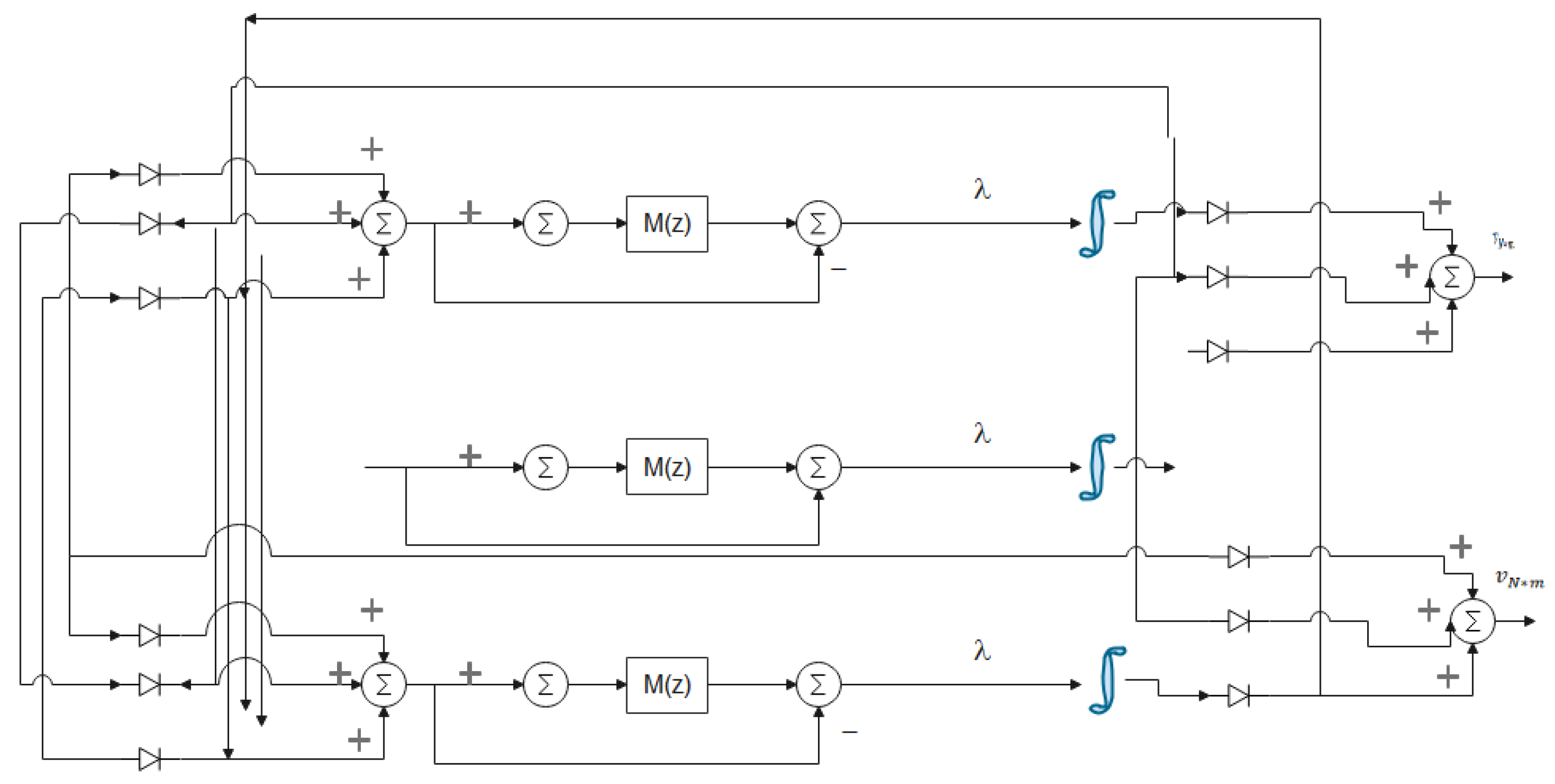
4. Real-Time Optimization Problem Using RNN

The global convergence and low complexity of RNN for optimization of linear models, constrained linear models, linear models with uncertainty, and various nonlinear models are represented in the literature. In this study, RNN optimizes a real-time QP problem enjoying parallel computation. To begin with, the original optimization problem is required to transform into a standard form. The input-state relationship of Equation (1) can be expressed in the following form:
x ( k + 1 ) = A ( p ( k ) ) x ( k ) + B ( p ( k ) ) u ( k ) + d ( p ( k ) )
The vectors of predicted outputs, inputs, and disturbance are as follows:
X ( k ) = [ X ( k + 1 ) X ( k + N ) ] T m × N U ( k ) = [ u ( k ) u ( k + N 1 ) ] T n × N D ( k ) = [ d ( k + 1 ) d ( k + N ) ] T o × N
where m ,   n , and o are the number of states, inputs, and disturbances, respectively. The predicted states can be easily shown to be in the following form:
X ( k + j ) = G ( p ( k + j 1 ) ) X ( k + j 1 ) + F ( p ( k + j 1 ) ) U ( k + j 1 ) + D ( k + j 1 ) , j = 1 , , N G ( p ( k ) ) = [ A ( p ( k ) )   A ( p ( k ) ) 2   A ( p ( k ) ) N ] T F ( p ( k ) ) = [ B ( p ( k ) )   A ( p ( k ) ) B ( p ( k ) ) + B ( p ( k ) ) A ( p ( k ) ) N 1 B ( p ( k ) ) + + A ( p ( k ) ) B ( p ( k ) ) + B ( p ( k ) ) ]
The constraints (2) can be represented as follows:
u m a x u ( k )   u m a x Δ u m a x u ( k ) u ( k 1 )   Δ u m a x x m a x G u + F + d   x m a x  
The optimization problem (16) can be written as follows:
min U X T Q ¯ X + U T R U = min U ( G X + F U + D ) T Q ¯ ( G X + F U + D ) + U T R U min U U T × ( ( F U ) T Q ¯ ( F U ) + R ) × U + ( G X + F U ) T Q ¯ ( G X + F U )
where
Q ¯ = [ Q 0 0 Q p ]
According to Equations (35) and (36), the standard form can be expressed as follows:
min v 1 2 v T H v + b T v Subject   to   T v q
where
H = 2 × ( ( F U ) T Q ¯ ( F U ) + R ) b = 2 × ( G X + F U ) T Q ¯ ( G X + F U ) T = [ I n × n I n × n I n × n I n × n G G ] ,   q = [ u m a x u m a x Δ u m a x + u ( k 1 ) Δ u m a x u ( k 1 ) X m a x F d X m a x + F + d ]
Remark 1.
The vector q is unknown as d is not measurable, while it can be estimated by the difference between the measured output and model output. In Reference [31], a simple model to find unknown parameters is proposed.
Remark 2.
In References [25,31], a simplified form of a dual neural network is described to ensure the lower computational burden by defining the dual form of the optimization problem (37) as follows:
State equation:
d ω d t = λ ( T H 1 T T ω + M ( T H 1 T T ω T H 1 c ω ) + T H 1 c )
where ω is the state variable of the network, λ > 0 adjusts the convergence rate of RNN, and M is a piecewise linear function as follows:
M ( z ) = { q m i n                                                   z < q m i n z                                   q m i n < z < q m a x q m a x                                                 z > q m a x  
Output equation:
v = H 1 T T ω H 1 c
In the dual form of the optimization problem, constraints are added to the primary cost function as a penalty term. This means that, if T v < q , the cost function decreases by a factor of α ; otherwise, for T v > q , the cost function is penalized. The single-layer RNN is given in Figure 1. The global convergence of the proposed network is verified in [31].
Finally, the proposed MPC algorithm can be summarized in the following steps:
  • The value of Q ,   R , λ , N , u m a x , y m a x , d m a x , p and model ( A , B ) ;
  • Specify K using (12) and θ using (15);
  • Repeat the procedure of finding u ( k ) by solving Equations (38)–(40).
The whole procedure is also depicted in Figure 2.

5. Case Study

Alkylation of benzene with ethylene, a principal process in the petrochemical industry, produces ethylbenzene, which is widely used as a large-scale benchmark. As shown in Figure 3, the process studied in this work consists of four continuously stirred tank reactors (CSTRs) and a flash tank separator. A detailed description of the process is described in [32,33]. The process’s manipulated variables are heat inputs to five vessels shown by Q1, Q2, Q3, Q4, and Q5. The temperatures of five vessels T1, T2, T3, T4, and T5 are considered the process’s outputs. The process’s dynamic behavior is set out in detail in Equations (41)–(45), and all parameters are named in Table 1. For more information and the value of fixed parameters, refer to [34].
d T 1 d t = Q 1 + F 1 C A 0 H A ( T A 0 ) + F 2 C B 0 H B ( T B 0 ) + i A , B , C , D F r 2 C i r H i ( T 4 ) F 3 C i 1 H i ( T 1 ) i A , B , C , D C i 1 C p i V 1 + Δ H r 1 r 1 ( T 1 , C A 1 , C B 1 ) Δ H r 2 r 2 ( T 1 , C B 1 , C C 1 ) i A , B , C , D C i 1 C p i
d T 2 d t = Q 2 + F 4 C B 0 H B ( T B 0 ) + i A , B , C , D F 3 C i 1 H i ( T 1 ) F 5 C i 2 H i ( T 2 ) i A , B , C , D C i 2 C p i V 2 + Δ H r 1 r 1 ( T 2 , C A 2 , C B 2 ) Δ H r 2 r 2 ( T 2 , C A 2 , C B 2 ) i A , B , C , D C i 2 C p i
d T 3 d t = Q 3 + F 6 C B 0 H B ( T B 0 ) + i A , B , C , D F 5 C i 2 H i ( T 2 ) F 7 C i 3 H i ( T 3 ) i A , B , C , D C i 3 C p i V 3 + Δ H r 3 r 1 ( T 3 , C A 3 , C B 3 ) Δ H r 3 r 2 ( T 3 , C B 3 , C C 3 ) i A , B , C , D C i 3 C p i
d T 4 d t = Q 4 + i A , B , C , D F 7 C i 3 H i ( T 3 ) + F 9 C i 5 H i ( T 5 ) i A , B , C , D C i 4 C p i V 4 + i A , B , C , D M i H i ( T 4 ) F 8 C i 4 H i ( T 4 ) M i H v a p i i A , B , C , D C i 4 C p i V 4
d T 5 d t = Q 5 + F 10 C D 0 H D ( T D 0 ) + i A , B , C , D F r 1 C i r H i ( T 4 ) F 9 C i 5 H i ( T 5 ) i A , B , C , D C i 5 C p i V 5 + Δ H r 2 r 2 ( T 5 , C B 5 , C C 5 ) Δ H r 3 r 3 ( T 5 , C A 5 , C D 5 ) i A , B , C , D C i 5 C p i
The steady-state values of inputs and outputs and initial conditions are indicated in Table 2. The controller desires to steer the system from this initial condition to the steady- states condition while satisfying the constraints:
| Q 1 Q 1 s | < 7.5 × 10 5 ,   | Q 2 Q 2 s | < 5 × 10 5 ,   | Q 3 Q 3 s | < 5 × 10 5 | Q 4 Q 4 s | < 6 × 10 5 ,   | Q 5 Q 5 s | < 5 × 10 5
In contrast to previous works that developed nonlinear MPC and/or noncentralized MPC, an MPC setup built on the LPV model, improved by RNN, is proposed in this paper, having lower complexity and better performance. More significantly, F r , C C 0 , and C D 0 are considered to be time-varying, for the first time, to the best of the authors’ knowledge. From a practical point of view, these variables are selected to be scheduling variables with ± 10 % variation around their nominal values. Before applying the controller, the LPV-IO framework is required to be identified so that ten levels are defined within the range of 90% to 110% of the nominal value for each scheduling variable. The global LPV model originates from a polynomial interpolation of ten local LTI models, identified with 500 data points in each level (operating condition). Each local model has five inputs and five outputs. All manipulated inputs are chosen to be pseudorandom binary signals to extract data with a sampling time of T = 10   s . With the measured data, the LTI models, afterward, are identified using MATLAB system identification Toolbox. With several simulations, it has been realized that a third-degree polynomial interpolation produced a good fit for constructing the global LPV-IO model, while the order of local transfer functions varies from second to fifth.
The scheduling variables and the responses that come from the global LPV-IO model and nonlinear model are presented in Figure 4 and Figure 5, respectively. The figures supplied show that the identified LPV model can predict the nonlinear system’s behavior. Moreover, mean square error (MSE) and Akaike’s final prediction error (FPE) for the global model were 0.032 and 0.058 in succession, and for the local LPV models, the range of MSE was between 0.004 and 0.062, and FPE changed from 0.040 to 0.081. Figure 5 and the numerical results show that the LPV-IO model is sufficiently reliable for estimating responses.

6. Results and Discussion

In the next step, the performance of the controller in terms of setpoint tracking and disturbance rejection is investigated, in which a step change at t = 1500 s with amplitude 2 × 10 3 is made in F 1 and F 2 . The controller parameters were N = 6 ,   Q = 1000 × I 5 × 5 ,   R = 10 7 × I 5 × 5 , and λ = 3.5 . All controllers employed in the performed comparison used the same parameters. The proposed approach is compared with linear RMPC [35], and the LPV controller studied in [17] is shown in Figure 6, where the dashed red line denotes the references, the blue line is the proposed method, the green line is linear RMPC, and the black line is LPV-IO RMPC. In all methods, MPC parameters are chosen according to [36,37].
Looking firstly at reference tracking, the proposed controller’s rise time is slightly larger than other methods, while being fast enough. On the other hand, the proposed controller has a lower settling time. In contrast to LPV-MPCs that reach the reference, the linear RMPC has a non-zero steady-state error, especially in T 4 and T 5 . The proposed controller reached the setpoint without any oscillations, while linear RMPC and LPV-RMPC suffer from large-amplitude oscillations. The reason behind the fluctuation in T 5 for linear RMPC can be found in Equation (35), such that C D 0 directly affects the output, and LRMPC failed to tackle the changes in molar densities of pure D. In general, regardless of rise time, settling time, and overshoot, all three methods followed the setpoints for T 1 to T 4 .
Turning to disturbance rejection, the studied approach outperforms others with removing the disturbance in a short time ranging from 120 s to 355 s for T 1 to T 5 . After time t = 1500 s, when the disturbance was applied to the process, the LRMPC violated both inputs and outputs constraints, especially in T 1 , although it can overcome the disturbances after a while; on the other hand, LPV-RMPC became highly unstable. Therefore, LPV-RMPC failed to cope with disturbances imposing the process in contrast to other methods, and high amplitude of oscillation in the LRMPC response can be devastating.
Regarding the cost function, the wasted resources by LPV-RMPC are 5.04 times more than LRMPC and 1.59 × 10 times greater than those of the proposed method, which proved that the studied approach is significantly cost-effective. More importantly, the cost function of LRMPC and LPV-RMPC did not converge to zero, so that they cannot deal with changes in three scheduling variables. The MSE of all three methods for different outputs is reported in Table 3. Using the proposed method leads to a sharp decline in error compared with other methods, as the MSE for LRMPC, LPV-RMPC, and proposed method were 447.56, 5.09 × 10³, and 43.84, respectively. In short, the proposed method had an acceptable speed (rise time, settling time, and time required to remove disturbance), as well as lower MSE and cost.
After evaluating the performance of the proposed controller, the importance of RNN needs to be emphasized. Finding the global minimum in a shorter time was the primary reason behind using RNN in this study. To this end, RNN is compared with three widely used optimization algorithms for MPCs, namely, sequential quadratic programming (SQP), genetic algorithm (GA), and singular value decomposition (SVD). It has been proven that using RNN reduces the average time required for computing the control action in each sampling in contrast with NMPC based on SQP, GA, and SVD. The average run-time and MSE of these methods is reported in Table 4 and Figure 7, Figure 8 and Figure 9. The RNN-based method experienced far less MSE (43.84) and cost ( 2.03 × 10 4 ) than other optimization algorithms and found the optimal control actions remarkably quick (0.033). GA ranked second in cost and MSE, while being slow, resulting in instability and significant fluctuations in some simulations. In stark contrast, however, SVD has faster responses, although it failed to converge the minimum cost function at times and saw monumental errors. SQP, on the other side, had a smaller MSE and cost than SVD and solved the optimization problem in a shorter time than GA did. According to Figure 7, RNN and SVD have the lowest and highest MSE, respectively. Figure 8 depicts that SQP and GA are sluggish as opposed to RNN and SVD. As described in Figure 9, SVD is the only method with a significant error and fails to find the proper control actions from the optimization problem.

7. Conclusions

An RMPC with an LPV-IO model is investigated in this paper, in which an RNN algorithm solves the real-time optimization problem. The study had three contributions. Firstly, an RNN-based optimization algorithm was developed to offer global convergence and lower the online computational load. Secondly, free control moves were added to the constant control gain to maintain the closed-loop stability when facing bounded disturbances. Lastly, concerning previous studies for MPC with LPV, the proposed method inherently enjoys a shrunken conservatism degree owing to finding the larger possible terminal region, using free control moves, and the global solution of the optimization problem.
This approach’s effectiveness was monitored and compared with LRMPC [35] and LPV-RMPC [17] in an alkylation of benzene process, nonlinear, and large-scale with three scheduling variables. The proposed method was astonishingly successful in both setpoint tracking and disturbance rejection having a reasonable rise time, settling time, MSE, and response amplitude. The LRPMC had a similar speed response while suffering from adverse oscillation. The LPV-RMPC can partially track the predefined reference outputs, whereas it failed to remain stable when facing disturbances. Meanwhile, four optimization algorithms are utilized to solve the online optimization problem of the proposed controller. The results showed that RNN and GA outdid in error reduction and finding the optimal solution; nonetheless, GA was sluggish, and thus detrimental to stability. SVD had the fastest convergence rate with the highest MSE and cost value, and SQP, with a stable response, had the worst execution with an excellent average time and MSE. Future works will focus on showing the stability of the LPV-IO system with multiplicative disturbances. Moreover, the conservatism can be further lowered by ellipsoidal invariant sets with polyhedral invariant sets.

Author Contributions

Conceptualization, M.H., A.R. and W.Z.; methodology, M.H.; software, M.H.; validation, M.H., A.R. and W.Z.; formal analysis, M.H.; investigation, M.H.; resources, M.H., A.R. and W.Z.; writing—original draft preparation, M.H.; writing—review and editing, M.H., A.R. and W.Z.; visualization, M.H.; supervision, A.R. and W.Z.; project administration, A.R. and W.Z. All authors have read and agreed to the published version of the manuscript.

Funding

This research received no external funding.

Conflicts of Interest

The authors declare no conflict of interest.

References

  1. Camacho, E.F.; Alba, C.B. Model Predictive Control; Springer Science & Business Media: Berlin, Germany, 2013. [Google Scholar]
  2. Yaramasu, V.; Wu, B. Model Predictive Control of Wind Energy Conversion Systems; John Wiley & Sons: Hoboken, NJ, USA, 2016. [Google Scholar]
  3. Raković, S.V.; Levine, W.S. Handbook of Model Predictive Control; Springer: Berlin/Heidelberg, Germany, 2018. [Google Scholar]
  4. Zhang, R.; Xue, A.; Gao, F. Model Predictive Control; Springer Science and Business Media LLC: Berlin, Germany, 2019. [Google Scholar]
  5. Morato, M.M.; Normey-Rico, J.E.; Sename, O. Model predictive control design for linear parameter varying systems: A survey. Annu. Rev. Control. 2020, 49, 64–80. [Google Scholar] [CrossRef]
  6. Yu, S.; Böhm, C.; Chen, H.; Allgöwer, F. Model predictive control of constrained LPV systems. Int. J. Control 2012, 85, 671–683. [Google Scholar] [CrossRef]
  7. Yang, Y.; Ding, B. Model predictive control for LPV models with maximal stabilizable model range. Asian J. Control 2020, 22, 1940–1950. [Google Scholar] [CrossRef]
  8. Hu, C.; Wei, X.; Ren, Y. Passive fault-tolerant control based on weighted LPV tube-MPC for air-breathing hypersonic vehicles. Int. J. Control Autom. Syst. 2019, 17, 1957–1970. [Google Scholar] [CrossRef]
  9. Wang, X.; Zhang, X.; Yang, X. Delay-dependent robust dissipative control for singular LPV systems with multiple input delays. Int. J. Control Autom. Syst. 2019, 17, 327–335. [Google Scholar] [CrossRef]
  10. Abbas, H.S.; Toth, R.; Meskin, N.; Mohammadpour, J.; Hanema, J. A robust MPC for input-output LPV Models. IEEE Trans. Autom. Control 2016, 61, 4183–4188. [Google Scholar] [CrossRef]
  11. Ding, B.; Wang, P.; Hu, J. Dynamic output feedback robust MPC with one free control move for LPV model with bounded disturbance. Asian J. Control 2017, 20, 755–767. [Google Scholar] [CrossRef]
  12. Hu, J.; Ding, B. One-step ahead robust MPC for LPV model with bounded disturbance. Eur. J. Control 2020, 52, 59–66. [Google Scholar] [CrossRef]
  13. Alcalá, E.; Puig, V.; Quevedo, J.; Rosolia, U. Autonomous racing using linear parameter varying-model predictive control (LPV-MPC). Control Eng. Pract. 2020, 95, 104270. [Google Scholar] [CrossRef]
  14. Li, D.; Xi, Y. The feedback robust MPC for LPV systems with bounded rates of parameter changes. IEEE Trans. Autom. Control 2010, 55, 503–507. [Google Scholar]
  15. Xu, Z.; Zhao, J.; Qian, J.; Zhu, Y. Nonlinear MPC using an identified LPV model. Ind. Eng. Chem. Res. 2009, 48, 3043–3051. [Google Scholar] [CrossRef]
  16. Calderón, H.M.; Cisneros, P.S.; Werner, H. qLPV predictive control-A benchmark study on state space vs input-output approach. IFAC-Pap. 2019, 52, 146–151. [Google Scholar] [CrossRef]
  17. Abbas, H.S.; Hanema, J.; Tóth, R.; Mohammadpour, J.; Meskin, N. An improved robust model predictive control for linear parameter-varying input-output models. Int. J. Robust Nonlinear Control 2018, 28, 859–880. [Google Scholar] [CrossRef]
  18. Cisneros, P.S.G.; Werner, H. Stabilizing model predictive control for nonlinear systems in input-output quasi-LPV form. In Proceedings of the 2019 American Control Conference (ACC), Philadelphia, PA, USA, 10–12 July 2019; pp. 1002–1007. [Google Scholar]
  19. Bouzerdoum, A.; Pattison, T. Neural network for quadratic optimization with bound constraints. IEEE Trans. Neural Netw. 1993, 4, 293–304. [Google Scholar] [CrossRef]
  20. Tan, K.C.; Tang, H.; Yi, Z. Global exponential stability of discrete-time neural networks for constrained quadratic optimization. Neurocomputing 2004, 56, 399–406. [Google Scholar] [CrossRef]
  21. Xia, Y.; Wang, J. A recurrent neural network for nonlinear convex optimization subject to nonlinear inequality constraints. IEEE Trans. Circuits Syst. I Regul. Pap. 2004, 51, 1385–1394. [Google Scholar] [CrossRef]
  22. Xia, Y.; Feng, G.; Wang, J. A novel recurrent neural network for solving nonlinear optimization problems with inequality constraints. IEEE Trans. Neural Netw. 2008, 19, 1340–1353. [Google Scholar] [PubMed]
  23. Xia, Y.; Wang, J. A general projection neural network for solving monotone variational inequalities and related optimization problems. IEEE Trans. Neural Netw. 2004, 15, 318–328. [Google Scholar] [CrossRef] [PubMed]
  24. Nguyen, L.V.; Qin, X. Some Results on Strongly Pseudomonotone Quasi-Variational Inequalities. Set-Valued Var. Anal. 2019, 28, 239–257. [Google Scholar] [CrossRef]
  25. Pan, Y.; Wang, J. Model predictive control for nonlinear affine systems based on the simplified dual neural network. In Proceedings of the 2009 IEEE International Conference on Control Applications, St. Petersburg, Russia, 8–10 July 2009; pp. 683–688. [Google Scholar]
  26. Wu, Z.; Christofides, P.D. Optimizing process economics and operational safety via economic MPC using barrier functions and recurrent neural network models. Chem. Eng. Res. Des. 2019, 152, 455–465. [Google Scholar] [CrossRef]
  27. Lanzetti, N.; Lian, Y.Z.; Cortinovis, A.; Dominguez, L.; Mercangoz, M.; Jones, C. Recurrent neural network based MPC for process industries. In Proceedings of the 2019 18th European Control Conference (ECC), Naples, Italy, 25–28 June 2019; pp. 1005–1010. [Google Scholar]
  28. Wollnack, S.; Werner, H. LPV-IO controller design: An LMI approach. In Proceedings of the 2016 American Control Conference (ACC); Institute of Electrical and Electronics Engineers (IEEE), Boston, MA, USA, 6–8 July 2016; pp. 4617–4622. [Google Scholar]
  29. Morato, M.M.; Normey-Rico, J.E.; Sename, O. Novel qLPV MPC Design with Least-Squares Scheduling Prediction. IFAC Pap. 2019, 52, 158–163. [Google Scholar] [CrossRef]
  30. Zhang, S.; Dai, L.; Xia, Y. Adaptive MPC for constrained systems with parameter uncertainty and additive disturbance. IET Control Theory Appl. 2019, 13, 2500–2506. [Google Scholar] [CrossRef]
  31. Pan, Y.; Wang, J. A neurodynamic optimization approach to nonlinear model predictive control. In Proceedings of the 2010 IEEE International Conference on Systems, Man and Cybernetics; Institute of Electrical and Electronics Engineers (IEEE), Istanbul, Turkey, 10–13 October 2010; pp. 1597–1602. [Google Scholar]
  32. Salahshoor, K.; Hadian, M. A decentralized event-based model predictive controller design method for large-scale systems. Autom. Control. Inf. Sci. 2014, 2, 26–31. [Google Scholar]
  33. Liu, J.; Chen, X.; De La Pena, D.M.; Christofides, P.D. Sequential and iterative architectures for distributed model predictive control of nonlinear process systems. Part I: Theory. AIChE J. 2010, 56, 3148–3155. [Google Scholar]
  34. Kayacan, E.; Ramon, H.; Saeys, W. Distributed nonlinear model predictive control of an autonomous tractor–trailer system. Mechatronics 2014, 24, 926–933. [Google Scholar] [CrossRef]
  35. Hu, J.; Ding, B. Output feedback robust MPC for linear systems with norm-bounded model uncertainty and disturbance. Automatica 2019, 108, 108489. [Google Scholar] [CrossRef]
  36. Moradmand, A.; Dorostian, M.; Shafai, B. Energy scheduling for residential distributed energy resources with uncertainties using model-based predictive control. JEPE 2021, 132, 107074. [Google Scholar]
  37. Dorostian, M.; Moradmand, A. Hierarchical Robust Model-based Predictive Control in Supply Chain Management under Demand Uncertainty and Time-delay. In Proceedings of the 2021 7th International Conference on Control, Instrumentation and Automation (ICCIA), Tabriz, Iran, 23–24 February 2021; pp. 1–6. [Google Scholar]
Figure 1. Recurrent neural network (RNN) framework [31].
Electronics 10 01557 g001
Figure 2. The proposed approach flowchart.
Electronics 10 01557 g002
Figure 3. Flow diagram of alkylation of benzene process.
Electronics 10 01557 g003
Figure 4. Scheduling variables from left to right: F r (recycle flow rates), C C 0 (molar densities of pure C), and C D 0 (molar densities of pure D).
Electronics 10 01557 g004
Figure 5. Temperatures in five vessels: blue and red lines indicate the measured outputs and simulated outputs from the LPV model, respectively.
Electronics 10 01557 g005
Figure 6. The temperatures of vessels and cost function using three studied methods (dashed red line: references, the blue line: proposed method, the green line: linear RMPC, the black line: LPV-IO RMPC).
Electronics 10 01557 g006
Figure 7. MSE of different optimization algorithms.
Electronics 10 01557 g007
Figure 8. Average run-time of different optimization algorithms.
Electronics 10 01557 g008
Figure 9. The cost function of different optimization algorithms.
Electronics 10 01557 g009
Table 1. Process variables of the alkylation of benzene process.
VariablesDefinition
C A 1 , C B 1 , C C 1 , C D 1 Concentrations of A, B, C, D in CSTR-1
C A 2 , C B 2 , C C 2 , C D 2 Concentrations of A, B, C, D in CSTR-2
C A 3 , C B 3 , C C 3 , C D 3 Concentrations of A, B, C, D in CSTR-3
C A 4 , C B 4 , C C 4 , C D 4 Concentrations of A, B, C, D in Separator
C A 5 , C B 5 , C C 5 , C D 5 Concentrations of A, B, C, D in CSTR-1
C A r , C B r , C C r , C D r Concentrations of A, B, C, D in F r , F r 1 , F r 2
T 1 , T 3 , T 3 , T 4 , T 5 Temperatures in each vessel
T r e f Reference temperature
F 3 , F 5 , F 7 , F 8 , F 9 Effluent flow rates from each vessel
F 1 , F 2 , F 4 , F 6 , F 10 Feed flow rates to each vessel
F r , F r 1 , F r 2 Recycle flow rates
H v a p A , H v a p B , H v a p C , H v a p D Enthalpies of vaporization of A, B, C, D
H A r e f , H B r e f , H C r e f , H D r e f Enthalpies of A, B, C, D at T r e f
Δ H r 1 , Δ H r 2 , Δ H r 3 Heat of reactions 1, 2, and 3
V 1 , V 2 , V 3 , V 4 , V 5 Volume of each vessel
Q 1 , Q 2 , Q 3 , Q 4 , Q 5 External heat/coolant inputs to each vessel
C p A , C p B , C p C , C p D Heat capacity of A, B, C, D at liquid phase
α A , α B , α C , α D Relative volatilities of A, B, C, D
C A 0 , C B 0 , C C 0 , C D 0 Molar densities of pure A, B, C, D
T A 0 , T B 0 , T D 0 Feed temperatures of pure A, B, D
k Fraction of overhead flow recycled to the reactors
C A 1 , C B 1 , C C 1 , C D 1 Concentrations of A, B, C, D in CSTR-1
C A 2 , C B 2 , C C 2 , C D 2 Concentrations of A, B, C, D in CSTR-2
C A 3 , C B 3 , C C 3 , C D 3 Concentrations of A, B, C, D in CSTR-3
C A 4 , C B 4 , C C 4 , C D 4 Concentrations of A, B, C, D in Separator
C A 5 , C B 5 , C C 5 , C D 5 Concentrations of A, B, C, D in CSTR-1
C A r , C B r , C C r , C D r Concentrations of A, B, C, D in F r , F r 1 , F r 2
T 1 , T 3 , T 3 , T 4 , T 5 Temperatures in each vessel
T r e f Reference temperature
F 3 , F 5 , F 7 , F 8 , F 9 Effluent flow rates from each vessel
F 1 , F 2 , F 4 , F 6 , F 10 Feed flow rates to each vessel
F r , F r 1 , F r 2 Recycle flow rates
H v a p A , H v a p B , H v a p C , H v a p D Enthalpies of vaporization of A, B, C, D
H A r e f , H B r e f , H C r e f , H D r e f Enthalpies of A, B, C, D at T r e f
Δ H r 1 , Δ H r 2 , Δ H r 3 Heat of reactions 1, 2, and 3
V 1 , V 2 , V 3 , V 4 , V 5 Volume of each vessel
Q 1 , Q 2 , Q 3 , Q 4 , Q 5 External heat/coolant inputs to each vessel
C p A , C p B , C p C , C p D Heat capacity of A, B, C, D at liquid phase
α A , α B , α C , α D Relative volatilities of A, B, C, D
C A 0 , C B 0 , C C 0 , C D 0 Molar densities of pure A, B, C, D
Table 2. The steady-state and initial values.
Steady-State Temperatures of Vessels (K)Steady-State Inputs (J/K)Initial Temperatures of
Vessels (K)
T 1 s = 477.24 Q 1 s = 4.4 × 10 6 T 1 , 0 = 443.02
T 2 s = 476.97 Q 2 s = 4.6 × 10 6 T 2 , 0 = 437.12
T 3 s = 473.47 Q 3 s = 4.7 × 10 6 T 3 , 0 = 428.37
T 4 s = 470.60 Q 4 s = 9.2 × 10 6 T 4 , 0 = 433.15
T 5 s = 478.28 Q 5 s = 5.9 × 10 6 T 5 , 0 = 457.55
Table 3. The steady-state and initial values.
Method T 1 T 2 T 3 T 4 T 5 Total
LRMPC391.40387.25346.72331.76408.73347.56
LPV-RMPC 5.33 × 10 3 5.31 × 10 3 5.07 × 10 3 4.90 × 10 3 5.41 × 10 3 5.09 × 10 3
Proposed method67.3265.3052.3460.0076.4543.84
Table 4. A comparison of different optimization algorithms for finding the control signals.
Optimization AlgorithmMSEAverage TimeCost
RNN43.840.033 2.03 × 10 4
SQP153.120.76 8.04 × 10 6
GA76.550.81 5.01 × 10 4
SVD241.220.013 2.05 × 10 8
Publisher’s Note: MDPI stays neutral with regard to jurisdictional claims in published maps and institutional affiliations.

