Phaseless Characterization of Compact Antenna Test Range via Improved Alternating Projection Algorithm

Abstract

A practical compact antenna test range (CATR) requires good quiet zone quality for antenna characterization. This paper addresses the phase profile of the CATR quiet zone from the known intensity pattern of spatial domain and Fourier domain based on a combined alternating projection algorithm. The proposed algorithm is composed of Gerchberg–Saxton (GS) and Hybrid Input–Output (HIO) algorithms and the two algorithms with spatial phase perturbation (SPP) work collaboratively or independently under predesigned conditions. It is observed that the algorithm with random initial phase guess can always converge to an optimal solution by performing a series of hierarchical optimizations of the problem. The numerical results are in good agreement with simulated results in different frequency bands, overcoming the phase retrieval limitation of local convergence in the iterative process. Furthermore, to validate the effectiveness and robustness of the proposed procedure, the related discussions corresponding to different sampling areas in Fourier domain and different signal to noise ratios (SNRs) are given.

1. Introduction

With CATRs applied in the millimeter (mm) or sub-millimeter (submm) wave bands widely [1,2,3,4,5,6,7], increasing importance has been attached to the quiet zone disturbance assessment. In order to ensure effective CATR application, ±0.5 dB/±5° maximum amplitude/phase deviations from a constant value are allowed in the design and the implementation of a CATR. As is well known, due to variation of the temperature, probe positioning inaccuracy, and cable flexing, phase data acquisition becomes difficult, especially at mm- and submm- wave bands. Consequently, the phase retrieval (PR) of the field through amplitude-only has important research value. Additionally, the PR problem is of great concern in many other fields such as electron microscopy [8], astronomy [9], crystallography [10], lithography [11], optical imaging [12], and antenna characterization [13].

For simplicity, a very broad class of PR problems can be expressed as follows, $T\left[x(t)\right]=\left|y(w)\right|e^{j(w)}$. t and w denote coordinate vectors of object and observation domains, respectively. T is an operator, and $x(t)$ is an unknown signal. $|y(w)|$ is the amplitude of observation domain. Then, we find $x(t)$ from $|y(w)|$ and some a priori information. The alternating projection method known as an iteratively plane-to-plane backpropagation algorithm has been widely used. This class of methods originated from the classical Gerchberg–Saxton (GS) [14] algorithm where T is a Fourier transform operator. For the GS algorithm, the sets of attributes defined in the two domains are nonconvex, resulting in easily subject subjecting to trap into false solutions. For this reason, Fienup introduced a broad framework for iterative algorithms based on the GS algorithm in a series of papers, in which three main classes of algorithms, error-reduction (ER), basic input–output (BIO) as well as hybrid input-output (HIO), were proposed [15,16,17]. In addition, many modified methods based on the above alternating projection algorithms have been proposed for solving antenna phaseless measurement problems [18,19,20,21,22,23,24]. These methods retrieve phase information through two sets of amplitude. However, they are very sensitive to the initial phase guess. Besides, the size of each plane needs to be much larger than that of the required recovery aperture and the sampling rate should be at least $\lambda /4$.

Over the past few years, PhaseLift in a new PR framework provided by Candès [25,26] has been recently developed and has aroused widespread interest. Different from the alternating projection method for solving non-convex problems directly, the methods under the new framework rely on the relaxation of the original nonconvex problem into a convex one to get the global optimal solution. It is shown in PhaseLift [25,26] that lifting the PR problem to a higher dimensional and using semidefinite relaxation can transform the PR problem into a convex quadratic programming problem. When the measured signals are sparse signals, the stability of PhaseLift cannot be guaranteed. In order to improve the drawback, PhaseCut [27,28] was presented by accurately separating the amplitude and phase variables on the basis of PhaseLift. Due to the lifting, the two methods result in the prohibitive computational costs of two-dimensional signal reconstruction. Recently, a convex relaxation PhaseMax was proposed [29,30,31,32,33,34] to deal with a PR problem with non-lifting and operating in the original signal dimension. It is worth noting that convex relaxation methods require multiple sets of amplitude measurements in the observation domain to ensure convergence.

The other category of methods is usually based on minimization or maximization of some cost function or fitness function by global optimization procedures [35,36,37,38]. In [35], the weighted L2-norm regularize as a multiplicative constraint is introduced in the cost function, and the conjugate gradient method is employed to minimize the cost function. In [38], the gradient descent algorithm is utilized to minimize the cost function. Due to a lack of measured phase information, the overall cost function in these methods is non-linear, which usually fail to obtain the global optimal solution. Furthermore, these methods highly rely on the accuracy of the initial phase guess. If initial estimation is not reasonable, it is very difficult to obtain relatively accurate phase information. In [36], the method introduces a suitable relaxation in the cost function and decomposes the cost function maximization problem into a limited number of different convex programming problems. Nevertheless, the accuracy of this method is closely related to the number of unknowns. In [37], the cost function is minimized by the genetic algorithm. While the cost function contains two functions to accelerate the convergence of the algorithm, the algorithm still needs nearly 100,000 times to converge. More than this, the acquisition of two sets of amplitude information on different closed cylindrical surfaces will result in a higher cost than on planes.

While a number of phaseless antenna measurement approaches have been developed, there are very few papers concerning the phaseless characterization of quiet zone in CATR. In [38], the technique used to retrieve the phase of the quiet zone in CATR is based on a given initial phase range and two sets of amplitudes on the planes. The area of the plane is much larger than the aperture area of the main reflector; meanwhile, the least sampling interval needs to be $\lambda /4$. Even so, the measured surfaces still result in a truncation error inevitably. It should be noted that when there are many unknown parameters to be solved, it will converge to a false solution. In [39], we use the alternating projection method to recover the phase. However, four sets of amplitude data need to be sampled. Therefore, a large number of unknowns involved and the strict requirements for achievable measurement accuracy make the related PR problem of large electrically sized CATR still a very difficult task. To this end, we introduce a new alternating projection method to retrieve phase information of the quiet in CATR without relying on the accuracy of the initial phase guess.

In this paper, the proposed alternating projection method is based on the combination of GS and HIO algorithms with additional spatial phase perturbation (SPP) which allows to escape from the attraction region of one local optimum to that of another candidate solution. The novel algorithm is implemented in three parts. The first and second parts are a combination of the improved GS and HIO algorithms with the SPP and the third part is a pure improved HIO algorithm. This method takes advantage of the fact that the introduced SPP can allow simply skipping from one attraction area to another attraction area by simply changing the added interference phase. Meanwhile, the introduction of HIO in the third part of the algorithm is an attempt to prevent excessive interference when the solution is near the optimal solution because excessive interference may result in falling into the current local minimum solution of the problem.

The performance of this method has been pointed out by extensive numerical analysis which uses synthetic data to retain all the features of a CATR. The data is generated using MATLAB and commercial software GRASP-10.0 developed by TICRA. Referring to a Cassegrain Gregorian tri-reflection CATR with a spherical main reflector and two shaped sub-reflectors introduced in [5], problems related to the practical application and performance of this system have been pointed out.

2. Phase Retrieval as a Feasibility Problem

The image recovery problem in a Hilbert image space $\mathcal{L}$ is to estimate the original form x based on the measurements of the related physical image and some a priori information [40,41]. In the phase recovery problem of this article, the measurements are composed of two sets of amplitude data, which are the modulus s of the original signal x from the object domain and the modulus m of the Fourier transform $\widehat{x}$ of x, namely $\left|x\right|=s$ and $|\widehat{x}|=m$. The original signal $x\in C$ is complex value. The measurement data s and m are reals and nonnegative. Generally, we can properly model discrete physical signals/images in Hilbert signals/images space $\mathcal{L}$. Thus, a signal x in $\mathcal{L}$ is a square-integrable function, mapping a discrete variable to a complex number.

It is necessary to consider an important piece of information that the support of x is included in some set $D\subset {\mathrm{R}}^N$. Moreover, the complement of D is specified as $\complement D$. The characteristic functions of D and $\complement D$ are $1_D$ and $1_{\complement D}$, respectively, and the values of them are defined as

$$\begin{array}{c}\hfill 1_D(x)=\left\{\begin{array}{cc}1& \mathrm{if}x\in D\\ 0& \mathrm{if}x\in \complement D\end{array},\right.\end{array}$$

(1a)

$$\begin{array}{c}\hfill 1_{\complement D}(x)=\left\{\begin{array}{cc}0& \mathrm{if}x\in D\\ 1& \mathrm{if}x\in \complement D\end{array}.\right.\end{array}$$

(1b)

S and M are defined as the signal sets in $\mathcal{L}$ satisfying the constraints of the object domain constraint and the Fourier domain constraint, respectively. The object domain constraint restricts x to the set

$$\begin{array}{c}\hfill S=\left\{y\in \mathcal{L}\mid y·1_{\complement D}=0\mathrm{and}y⩾0\right\}.\end{array}$$

(2)

Meanwhile, the projection of a signal $x\in \mathcal{L}$ onto the object domain constraint S is given by

$$\begin{array}{c}\hfill P_S(x)=x·1_D.\end{array}$$

(3)

Since the measured amplitude s of the object domain is known, x can be defined by

$$\begin{array}{c}\hfill x(t)=\left\{{\displaystyle \begin{array}{cc}{\displaystyle s(t)\frac{x(t)}{|x(t)|}}& t\subset D\\ {\displaystyle x(t)}& \mathrm{otherwise}\end{array}.}\right.\end{array}$$

(4)

M is a signal set that satisfies the Fourier domain constraint, whose Fourier modulus is consistent with the modulus m, namely

$$\begin{array}{c}\hfill M=\{y\in \mathcal{L}||\widehat{y}\mid =m\},\end{array}$$

(5)

where $\widehat{y}$ denotes the Fourier transform of y, and is defined by

$$\begin{array}{c}\hfill {\displaystyle \widehat{y}(\omega )=\left\{{\displaystyle \begin{array}{cc}{\displaystyle m(\omega )\frac{\widehat{x}(\omega )}{|\widehat{x}(\omega )|}}& \mathrm{if}\widehat{x}(\omega )\ne 0\\ {\displaystyle m(\omega )}& \mathrm{otherwise}\end{array}.}\right.}\end{array}$$

(6)

It should be emphasized that M is closed but non-convex, whereas set S defined by Equation (2) is a closed convex set (as seen in [42]). The projection of a signal $x\in \mathcal{L}$ onto the Fourier magnitude constraint set M is to replace the amplitude of the Fourier transform of x with the known measured data m and inversely transform the result, and is expressed as

$$\begin{array}{c}\hfill P_M(x)={\mathcal{F}}^{-1}\left({\widehat{y}}_0\right).\end{array}$$

(7)

Therefore, the PR problem in Hilbert space can be expressed in mathematical form. This is to find a signal $x\in \mathcal{L}$ that satisfies the above constraint, namely

$$\begin{array}{c}\hfill \mathrm{find}x\in S\cap M.\end{array}$$

(8)

Through the mathematical formula, the problem of solving PR can be transformed into finding a suitable point in the intersection of two constraint sets. This kind of problem is called a feasibility problem in mathematical optimization. In addition, in this article we will only consider the phase recovery problem in the case of $S\cap M\ne ⌀$. Because the sampled signals are discrete signals with finite dimensions, the Hilbert space in this article can be equivalent to a Euclidean space whose dimension depends on the amount of data required to deal with the problem.

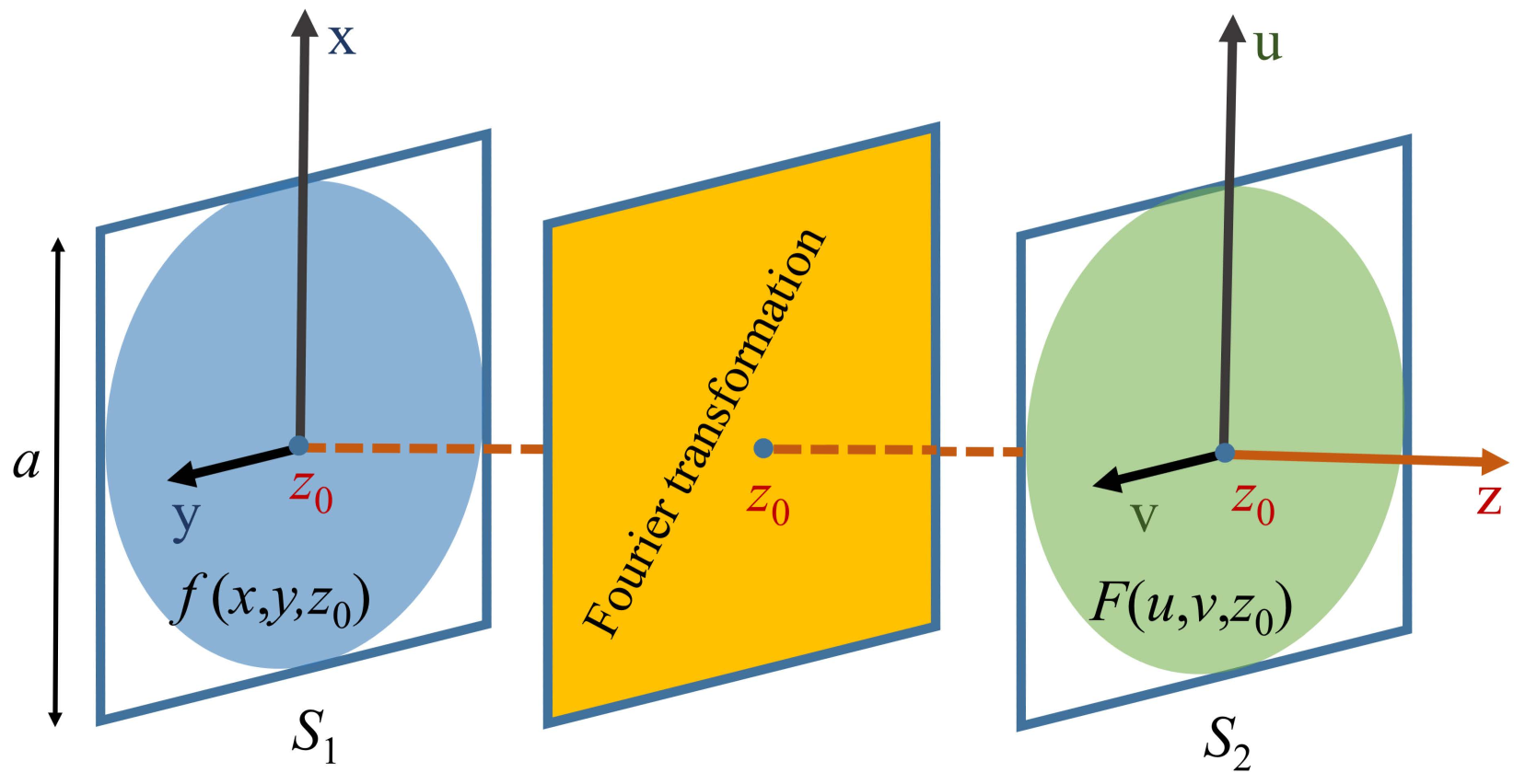
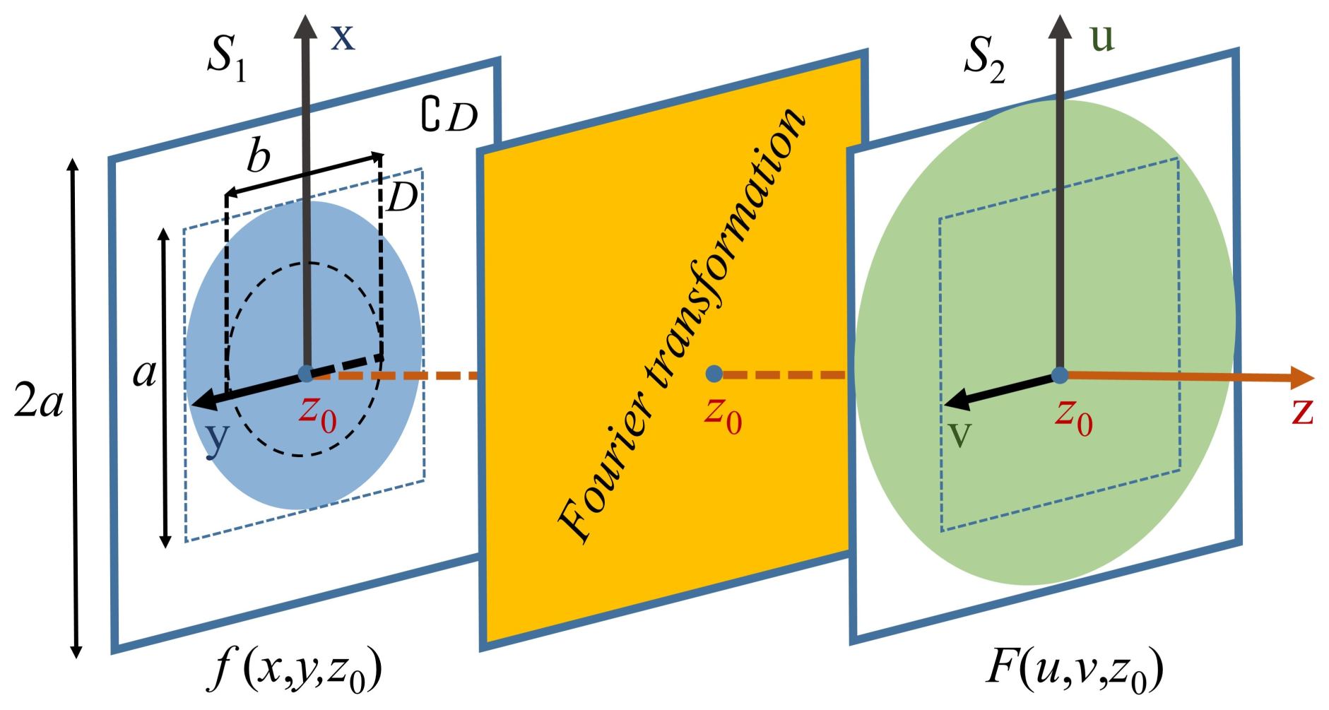
3. The Theory of Phase Retrieval of Quiet Zone

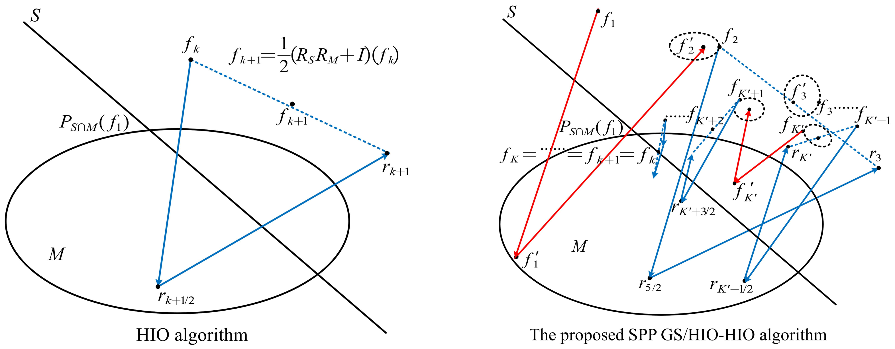
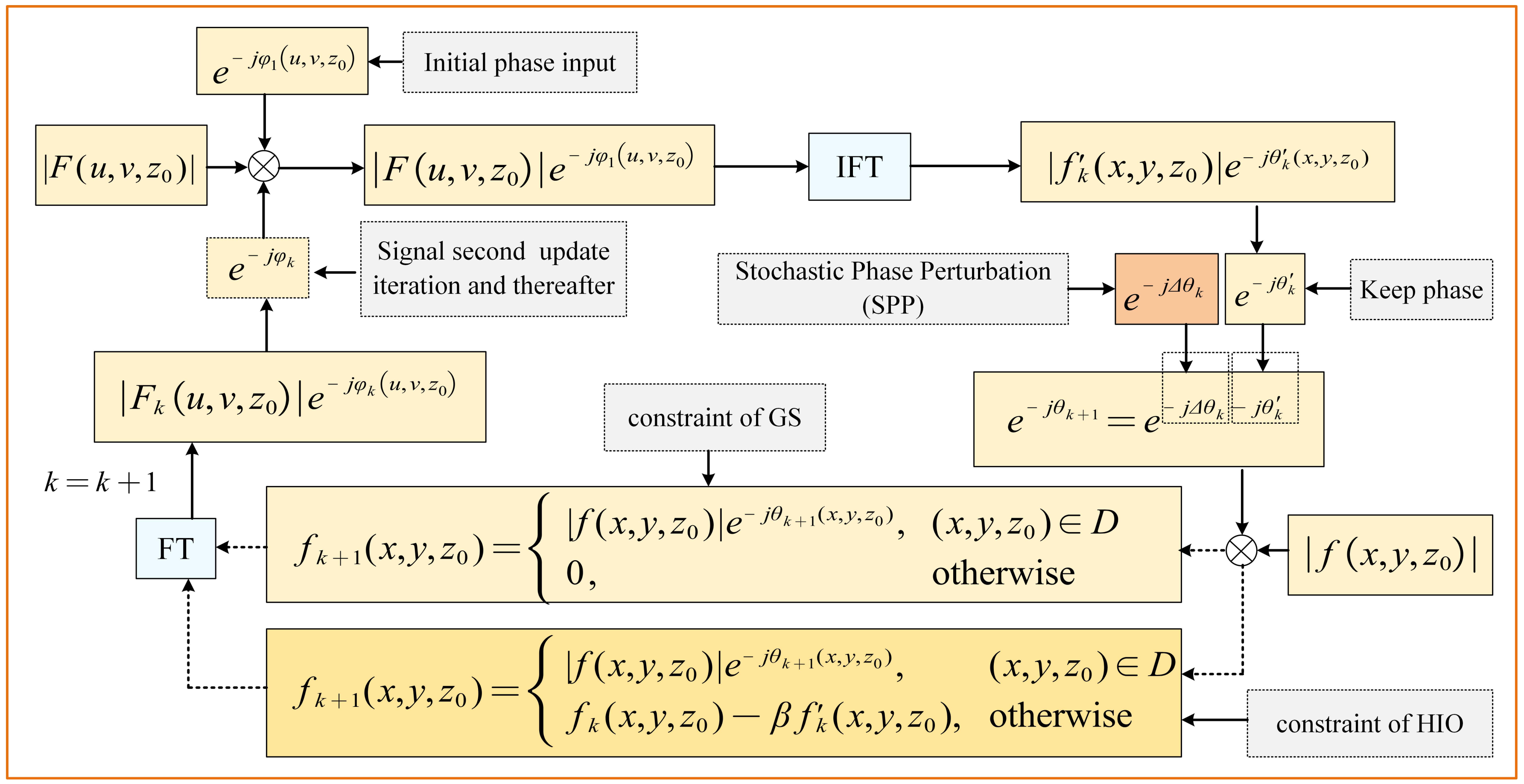
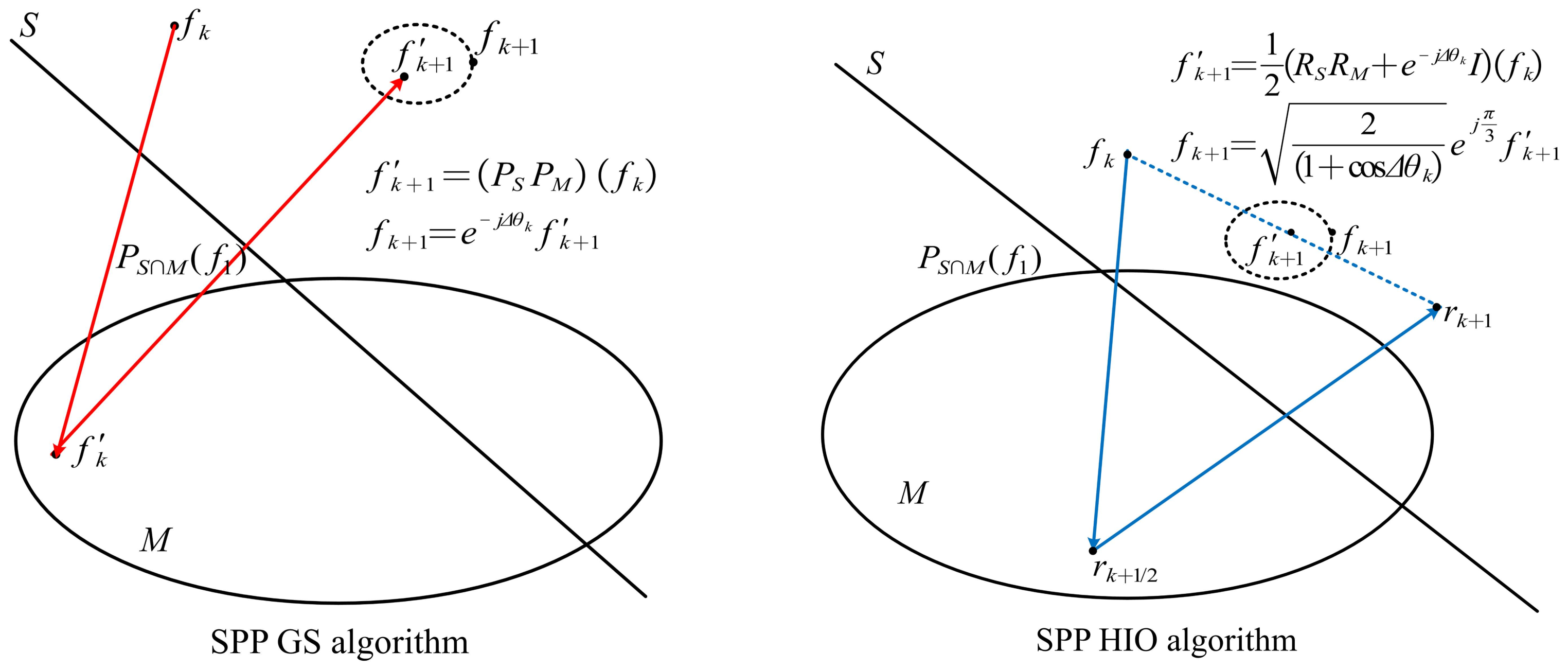
3.1. The Proposed SPP GS/HIO-HIO Algorithm

Let us consider the PR of the quiet zone in a Cartesian coordinate system Oxyz of a triple offset reflector CATR. The phase retrieval problem of the plane $S_1$ at $z=z_0$ with the transversal dimension $a\ast a$ in quiet zone can be solved when the amplitudes of the two planes $S_1$ and $S_2$ are measured as shown in Figure 1. The field of plane $S_2$ is the Fourier transform of the field of plane $S_1$ and this process can be achieved by a metasurface lens as explained in [43].

When alternating projection methods solve the feasibility problem of phase recovery, the signal is alternately projected onto the Fourier constraint set M and the object constraint set S to update until the algorithm converges and outputs the retrieved phase. If the update of the signal always satisfies the invariable constraint, the algorithm will not converge or fall into a local minimum corresponding to the “false solutions” of the problem. In order to avoid the shortages, the SPP GS/HIO-HIO algorithm proposed in this paper adaptively introduces different constraints to update the signal according to the process of dealing with the feasibility problem.

The process of the proposed SPP GS/HIO-HIO algorithm is shown in Figure 2. It can be mainly divided into the following three parts. The first part mainly uses the SPP GS algorithm to preprocess the signal. When the initial input signal consisting of a known amplitude and a randomly generated phase is projected onto the object domain, the constraint of SPP GS is performed to update the signal with the count number k increased by one. The second part is mainly to update the signal cyclically for $k_s-1$ times. Meanwhile, the constraint of SPP HIO is used to update the signal when it is projected onto the object domain under the condition of $\mathrm{mod}\left(k.k_s\right)>k_0$. The updated constraint of SPP HIO is replaced by that of SPP GS if $\mathrm{mod}\left(k.k_s\right)<k_0$, and then returned to the first part with the updated signal as the input value.

The addition of SPP in the first and second parts is to prevent the algorithm from failing to converge. However, extra interference effects in the presence of SPP will occur when the updated signal is close to the original target signal, which will also lead the algorithm to fall into a local minimum corresponding to the “false solutions” of the problem. Therefore, SPP will be removed on the condition of $k>K\prime$ in the third part. Moreover, the constraints for the signal updating in the object domain are those of the HIO algorithm. The retrieved phase of the updated signal will not successfully generate until the algorithm converges.

In order to prevent the occurrence of overlapping effects at the boundary, we additionally introduced the zero-padding method by adding equal zeros in both the x-direction and the y-direction, introduced in the object domain. As shown in Figure 3, the amplitudes of plane $S_1$ can be divided into two sets, set D and its complement $\complement D$ according to the zero region. The elements of set D are sampled amplitudes, while the elements of $\complement D$ are all padded with zeros. Furthermore, the sampled region in plane $S_2$ should cover the entire zero-padding part.

On the basis of the zero-padding method, we present in Figure 4 the flow chart of the signal updating with constraints of the SPP GS algorithm and the SPP HIO algorithm, respectively, when the signal is projected onto the object domain. The flow chart of the HIO algorithm is not given for the reason that it only lacks the addition of the SPP compared with that of the SPP HIO algorithm.

The equation of the control algorithm in the kth iteration update of the signal are

$$\begin{array}{cc}\hfill F_k(u,v,z_0)& =\left|F_k(u,v,z_0)\right|e^{-j{\phi }_k(u,v,z_0)}=\mathcal{F}\left\{f_k(x,y,z_0)\right\},\hfill \end{array}$$

(9a)

$$\begin{array}{c}\hfill F_k^{\prime }(u,v,z_0)=\left|F(u,v,z_0)\right|e^{-j{\phi }_k(u,v,z_0)},\end{array}$$

(9b)

$$\begin{array}{cc}\hfill f_k^{\prime }(x,y,z_0)& =\left|f_k^{\prime }(x,y,z_0)\right|e^{-j{\theta }_k^{\prime }(x,y,z_0)}={\mathcal{F}}^{-1}\left\{F_k^{\prime }(u,v,z_0)\right\}.\hfill \end{array}$$

(9c)

Equation (9) is where the signal $f_k(x,y,z_0)$ is projected onto the Fourier domain constraint set M to obtain $f_k^{\prime }(x,y,z_0)$. Then the signal $f_k^{\prime }(x,y,z_0)$ is projected onto the object domain constraint set S and updated to $f_{k+1}(x,y,z_0)$. According to the program process, the object domain constraint for signal updating will be different. When $k\le K^{\prime }$, SPP ($e^{-j\Delta {\theta }_k}$) is added and then $e^{-j{\theta }_{k+1}}=e^{-j\left(\Delta {\theta }_k+{\theta }_k^{\prime }\right)}$. If $mod\left(k,k_s\right)\le k_0$, $f_{k+1}(x,y,z_0)$ is defined as

$$\begin{array}{cc}\hfill & f_{k+1}(x,y,z_0)=\left\{\begin{array}{cc}|f(x,y,z_0)|e^{-j{\theta }_{k+1}(x,y,z_0)}& (x,y,z_0)\in D\\ 0& \mathrm{otherwise}\end{array},\right.\hfill \end{array}$$

(10)

If $mod\left(k,k_s\right)>k_0$, $f_{k+1}(x,y,z_0)$ is defined as

$$\begin{array}{cc}\hfill & f_{k+1}(x,y,z_0)=\left\{\begin{array}{cc}|f(x,y,z_0)|e^{-j{\theta }_{k+1}(x,y,z_0)}& (x,y,z_0)\in D\\ f_k(x,y,z_0)-\beta f_k^{\prime }(x,y,z_0)& \mathrm{otherwise}\end{array}.\right.\hfill \end{array}$$

(11)

When $k>K^{\prime }$, SPP is removed and then $e^{-j{\theta }_{k+1}}=e^{-j{\theta }_k^{\prime }}$; the signal updating is updated to

$$\begin{array}{cc}\hfill & f_{k+1}(x,y,z_0)=\left\{\begin{array}{cc}|f(x,y,z_0)|e^{-j{\theta }_k^{\prime }(x,y,z_0)}& (x,y,z_0)\in D\\ f_k(x,y,z_0)-\beta f_k^{\prime }(x,y,z_0)& \mathrm{otherwise}\end{array}.\right.\hfill \end{array}$$

(12)

As explained in [12], the phase $\Delta {\theta }_k(x,y)$ in SPP is expressed as:

$$\begin{array}{c}\hfill \Delta {\theta }_k(x,y,z_0)=\alpha \left(2{\left\{{\mathrm{rand}}_{(-1,1)}(x,y,z_0)\right\}}_k-1\right)(1-\frac{k}{K^{\prime }}).\end{array}$$

(13)

where $\alpha$ is a scaling factor that determines the initial size of the perturbation. In order to ensure that the introduced disturbance allows the algorithm to avoid converging to a local minimum, the initial value of perturbation cannot be selected as too small. The default value of $\alpha$ in this paper is set to $\pi /2$ unless otherwise specified. Moreover, $\left\{{\mathrm{rand}}_{(-1,1)}(x,y,z_0)\right\}$ is a randomly generated matrix at the $k\mathrm{th}$ iteration with the same dimensions as the plane $S_1$ being processed. The elements in the matrix are uniformly distributed between −1 and 1. The factor $\beta$ is a constant feedback parameter. It has been found that the value of $\beta$ between 0.5 and 1 can produce good results [44] and the value of $\beta$ is set to 1 in this paper.

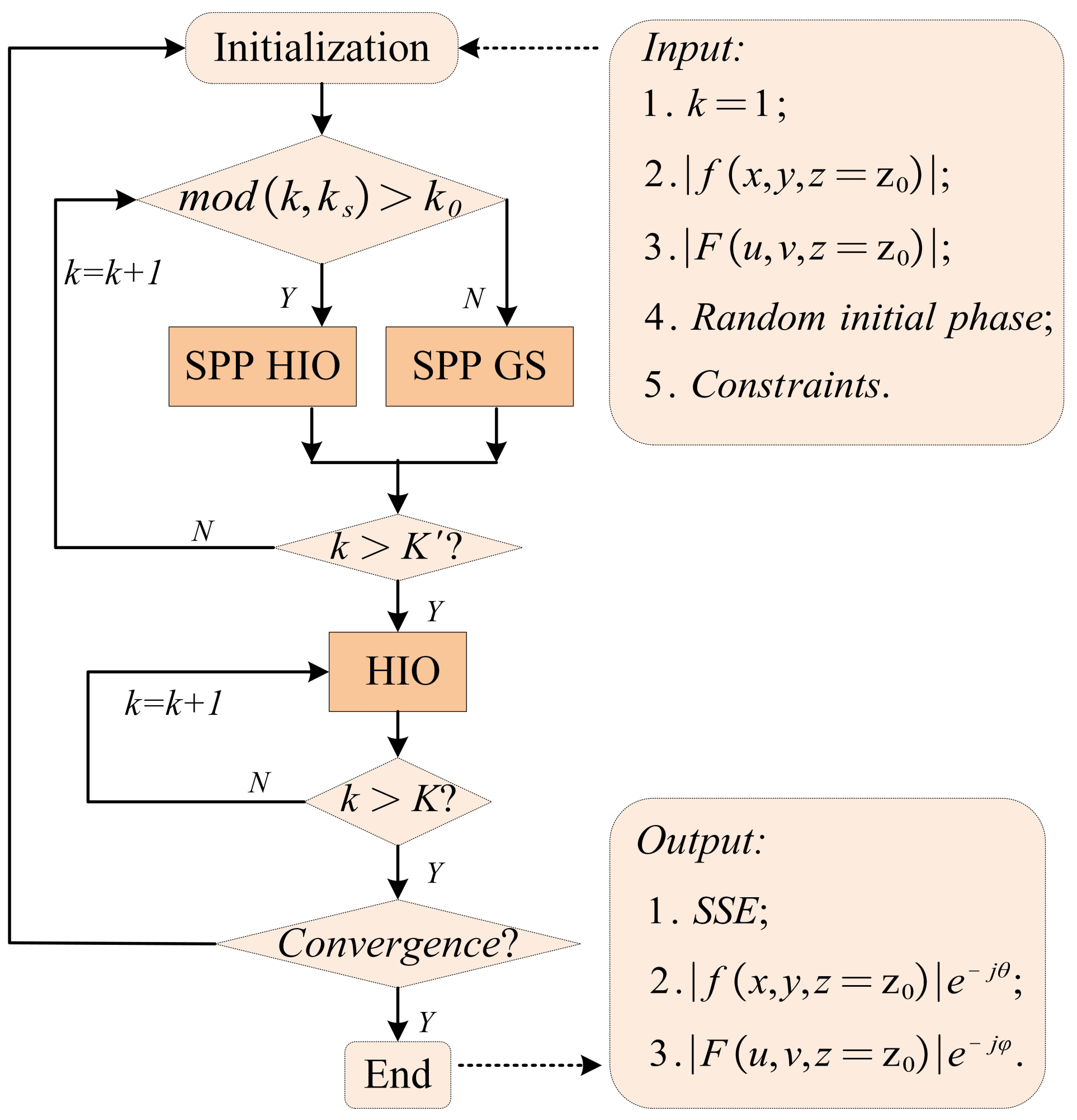
3.2. An Outline of the Solution Steps

The problem of PR has been transformed into a feasibility problem in mathematical optimization in Section 2. The main purpose for the optimization is to find a suitable signal in the intersection of two constraint sets. The following will explain in detail how the alternating projection algorithms work and the type of role that they play in the problem. For each update, the signal is first projected onto the Fourier-domain constraint set M and then onto the object-domain constraint set S. Furthermore, set S is convex (and actually linear) and closed, M is closed but nonconvex. The Fourier domain constraint remains the same throughout the solution. However, the support constraints contained in the object domain constraint set vary according to k.

When $k\le K^{\prime }$ and $mod\left(k,k_s\right)\le k_0$, the updated signal can be obtained through [45]

$$\begin{array}{cc}\hfill & f_{k+1}(x,y,z_0)=\left\{\begin{array}{cc}\left(P_M\left(f_k\right){\mathrm{e}}^{-j\Delta {\theta }_k}\right)(x,y,z_0),& \mathrm{if} \left(x,y,z_0\right)\in D\\ 0& \mathrm{otherwise}\end{array}.\right.\hfill \end{array}$$

(14)

Then, the signal can be further defined as

$$\begin{array}{c}\hfill f_{k+1}=e^{-j\Delta {\theta }_k}\left(P_S{P}_M\right)\left(f_k\right),\end{array}$$

(15)

For a better understanding, the projection process of the SPP GS method is shown in Figure 5.

When $k\le K^{\prime }$ and $mod\left(k,k_s\right)>k_0$, the support constraints for the signal updating will be changed as (16), which can be rewritten as (17).

$$\begin{array}{c}\hfill f_{k+1}(x,y,z_0)=\left\{\begin{array}{cc}\left(P_M\left(f_k\right)e^{-j\Delta {\theta }_k}\right)(x,y,z_0)& \mathrm{if} (x,y,z_0)\in D\\ f_k(x,y,z_0)-\beta \left(P_M\left(f_k\right)\right)(x,y,z_0)& \mathrm{otherwise}\end{array}\right.\end{array}$$

(16)

$$\begin{array}{cc}\hfill f_{k+1}& =1_D·P_M\left(f_k\right)e^{-j\Delta {\theta }_k}+1_{CD}·\left[f_k-\beta P_M\left(f_k\right)\right]\hfill \\ \hfill & =1_D·P_M\left(f_k(x,y,z_0)\right)e^{-j\Delta {\theta }_k}+\left(1-1_D\right)·\left[f_k(x,y,z_0)-\beta P_M\left(f_k\right)\right]\hfill \\ \hfill & =\left(P_S\left(\left(\beta +e^{-j\Delta {\theta }_k}\right)P_M-I\right)+\left(I-\beta P_M\right)\right)\left(f_k\right)\hfill \end{array}$$

(17)

$\beta$ is set to 1 in (17). Now let $R_S=\left(1+e^{-j\Delta {\theta }_k}\right)P_S-I$ and $R_M=\left(1+e^{-j\Delta {\theta }_k}\right)P_M-I$. Thus, the updated signal can be rewritten as (18).

$$\begin{array}{cc}\hfill f_{k+1}& =\left(P_S\left(\left(1+e^{-j\Delta {\theta }_k}\right)P_M-I\right)+\left(I-P_M\right)\right)\left(f_k\right)\hfill \\ \hfill & =\frac{1}{\left(1+e^{-j\Delta {\theta }_k}\right)}\left(\left(\left(1+e^{-j\Delta {\theta }_k}\right)P_S-I\right)\left(\left(1+e^{-j\Delta {\theta }_k}\right)P_M-I\right)+e^{-j\Delta {\theta }_k}I\right)\left(f_k\right)\hfill \\ \hfill & =\frac{1}{2}\sqrt{\frac{2}{\left(1+cos\Delta {\theta }_k\right)}}{e}^{j\frac{\pi }{3}}\left(R_S{R}_M+e^{-j\Delta {\theta }_k}I\right)\left(f_k\right)\hfill \end{array}$$

(18)

We can further simplify the form of (18) to obtain

$$\begin{array}{c}\hfill f_{k+1}=\frac{e^{j\frac{\pi }{3}}}{2}\sqrt{\frac{2}{\left(1+cos\Delta {\theta }_k\right)}}\left(R_S{R}_M+e^{-j\Delta {\theta }_k}I\right)\left(f_k\right).\end{array}$$

(19)

According to the form of (19), the corresponding signal projection and update can be divided into three steps through [46], shown in Figure 5. Firstly, calculate the reflection $r_{k+1/2}$ of $f_k$ in relation to set M, and then calculate the reflection $r_{k+1}$ of $r_{k+1/2}$ in relation to the set S. $f_{k+1}^{\prime }$ is the midpoint of the segment between $f_k$ and $r_{k+1}$. Finally, the updated $f_{k+1}$ can be obtained from (19).

If $k>K^{\prime }$, the perturbation phase $e^{-j\Delta {\theta }_k}$ will be removed, and the support constraint of the object domain set S for the signal updating is modified as (20), which can be simplified as follows:

$$\begin{array}{c}\hfill f_{k+1}(x,y,z_0)=\left\{\begin{array}{cc}\left(P_M\left(f_k\right)\right)(x,y,z_0)& \mathrm{if} (x,y,z_0)\in D\\ f_k(x,y,z_0)-\beta \left(P_M\left(f_k\right)\right)(x,y,z_0)& \mathrm{otherwise}\end{array}\right.\end{array}$$

(20)

$$\begin{array}{cc}\hfill f_{k+1}& =\left(P_S\left(2P_M-I\right)+\left(I-P_M\right)\right)\left(f_k\right)=\frac{1}{2}\left(\left(2P_S-I\right)\left(2P_M-I\right)+I\right)\left(f_k\right)\hfill \end{array}$$

(21)

Let $R_S=2P_S-I$ and $R_M=2P_M-I$; $f_{k+1}(x,y,z_0)$ can be expressed as

$$\begin{array}{c}\hfill f_{k+1}=\frac{1}{2}\left(R_S{R}_M+I\right)\left(f_k\right).\end{array}$$

(22)

The corresponding signal projection and update through (22) has been shown in Figure 6. Similarly, $r_{k+1/2}$($r_{k+1}$) is the reflection of $f_k$($r_{k+1/2}$) in relation to the set S (set M). $f_{k+1}$ is the midpoint of the segment between $f_k$ and $r_{k+1}$.

In this paper, the value of $k_0$, $k_s$, and $K^{\prime }$ are set to 1, 40, and 600, respectively. The number of updates k starts from 1, and the total number of updates K is set to 1200. The whole projection procedure of the proposed algorithm under these parameters is shown in Figure 6.

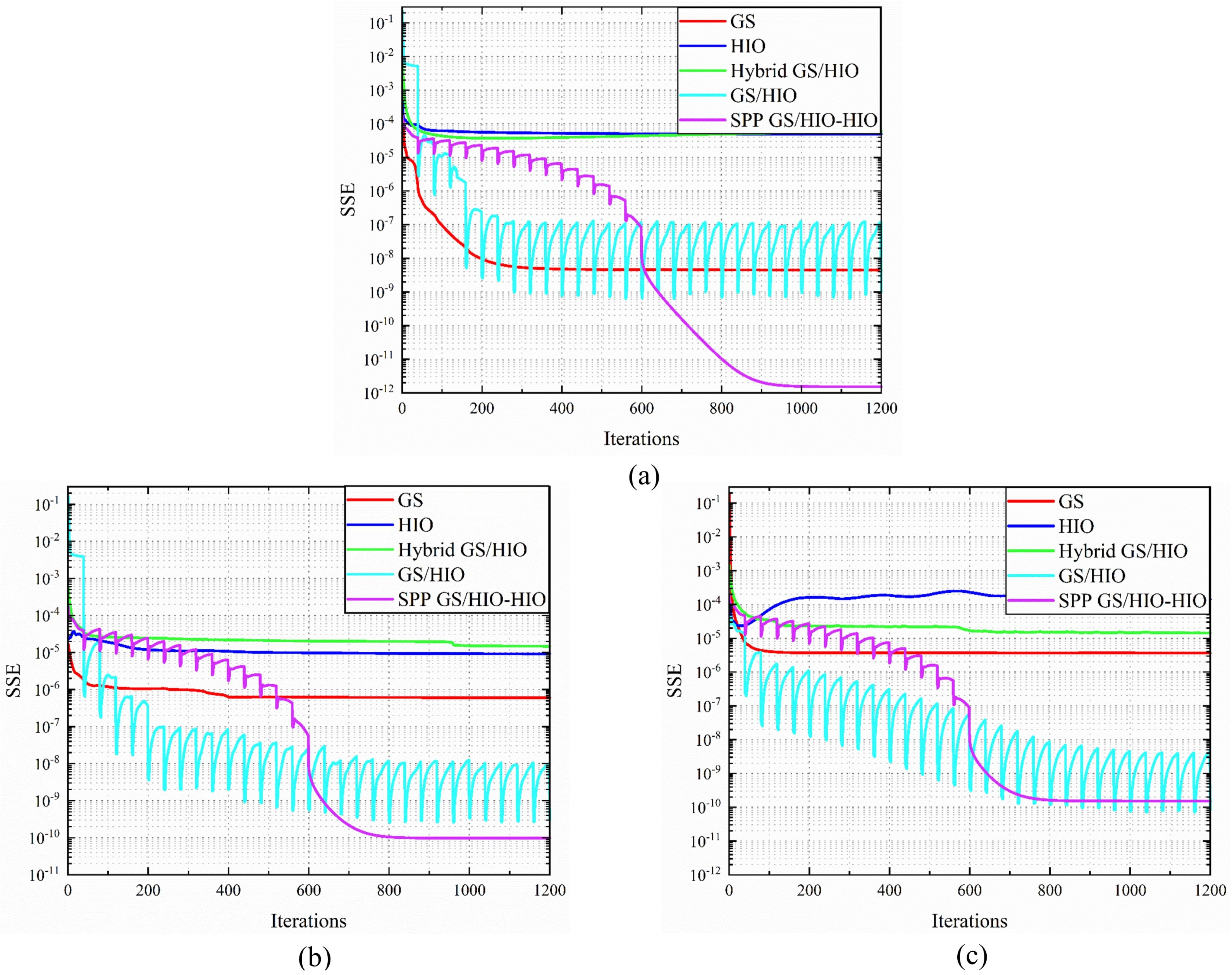
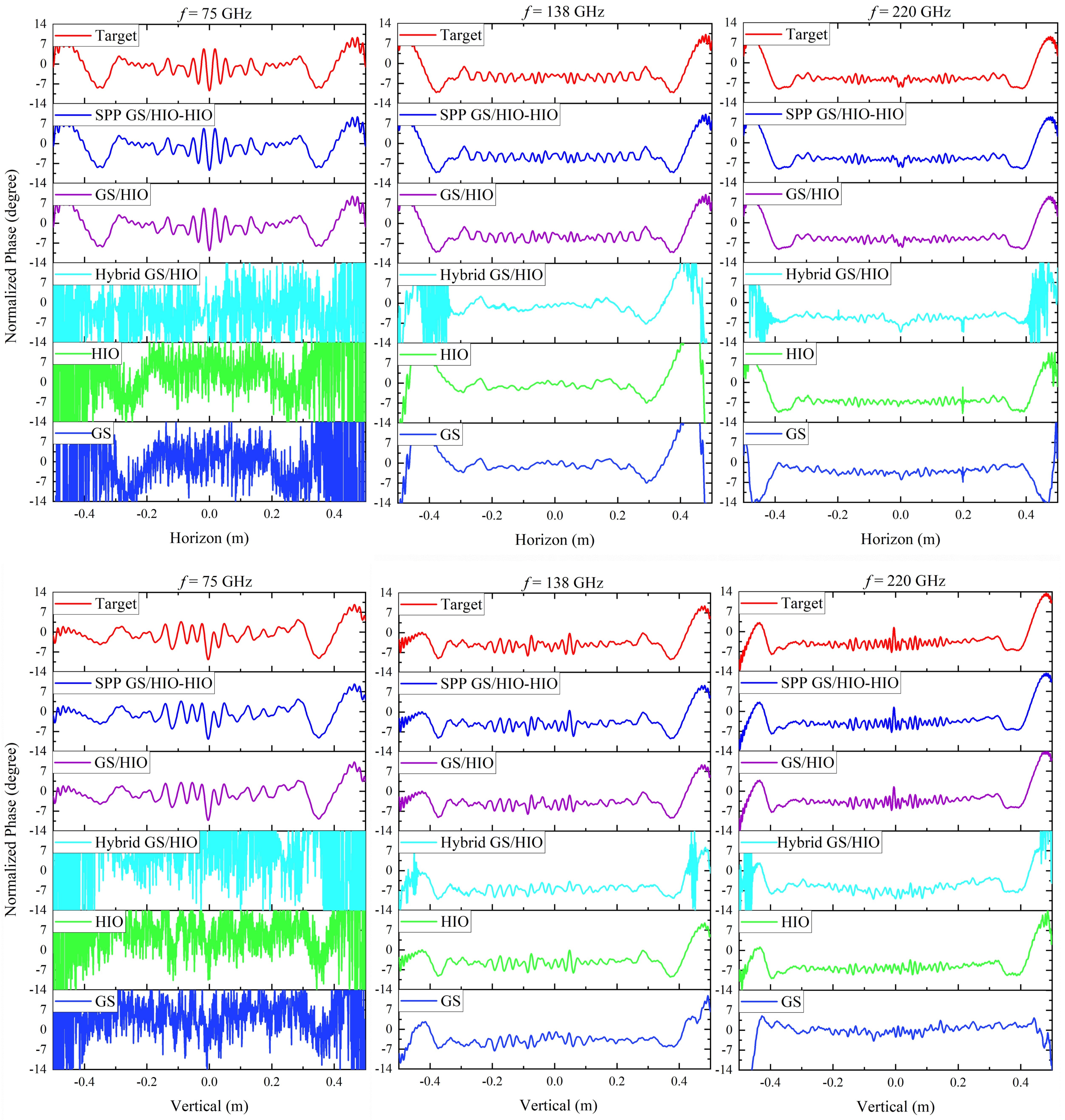
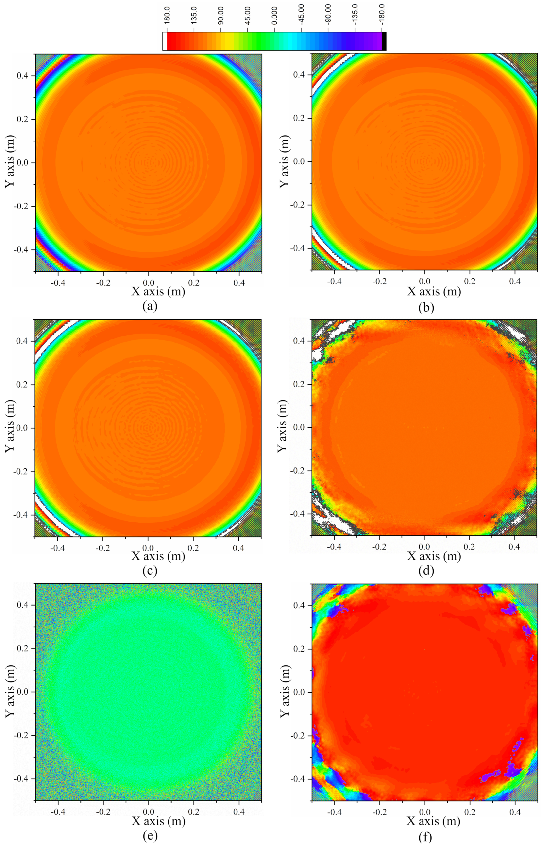
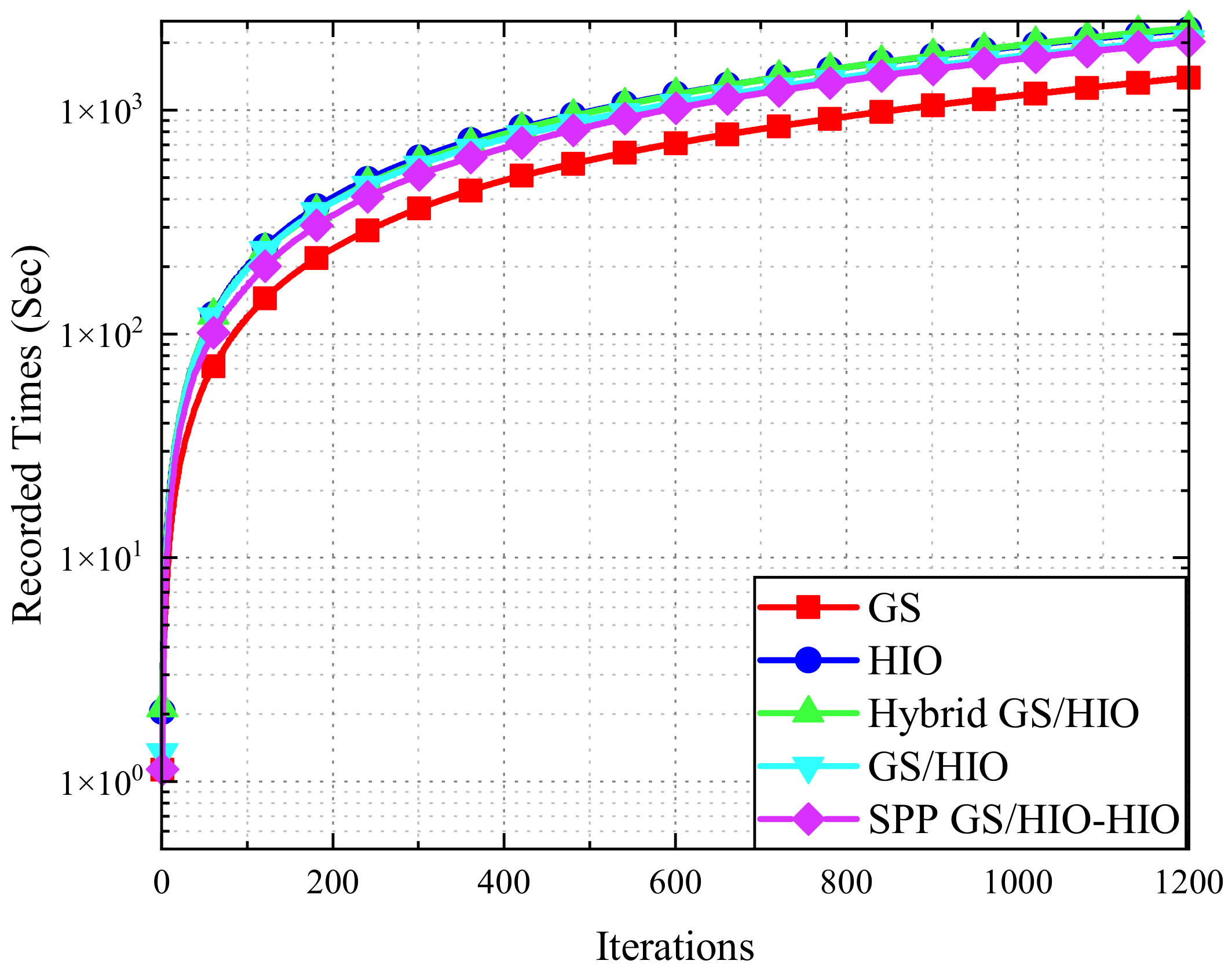
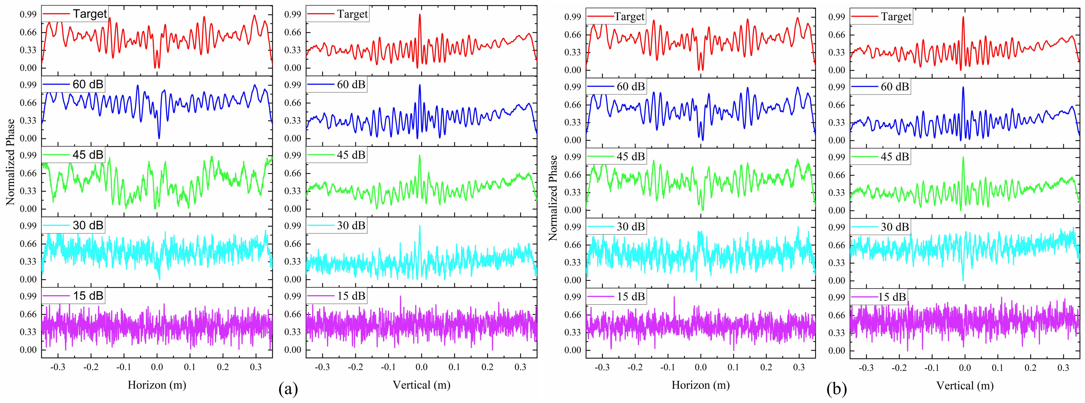
4. Numerical Verification of the Theoretical Results

Several numerical experiments have been performed to evaluate the effectiveness and stability of the algorithm in the proposed Cassegrain Gregorian tri-reflection CATR [5]. The CATR consists of a spherical main reflector with a circular aperture, two shaped sub-reflectors and a Gaussian feed horn as shown in Figure 7. The aperture diameter of the main reflector is a ($a=$ 1 m), and the diameter of the cross section of the effective quiet zone is b ($b=$ 0.7 m). For the sake of simplicity, set the z-axis coordinate of the plane of the quiet zone to be retrieved in this paper to $z_0$ (see in Figure 3).

The measurement planes $S_1$ and $S_2$ are sampled at $\lambda /2$ by commercial software GRASP-10 and MATLAB simulation software, respectively. If we want to obtain the missing phase of the plane with a diameter of a, the sampling areas of $S_1$ and $S_2$ are $a\ast a$ and $2a\ast 2a$, respectively. In order to assess the stability of the proposed approach, the missing phases of the $S_1$ with the CATR working at 75 GHz, 138 GHz, and 220 GHz, respectively, were recovered. Additionally, under the same initial input and total number of iterations ($K=1200$), the recovery performance of the proposed algorithm is compared with that of the other four algorithms: GS, HIO, GS/HIO [12], and hybrid GS/HIO [47] algorithms.

Before describing the details of PR, some explanations on performance indicators are needed. The discrete sum squared error (SSE) between the amplitude of the Fourier transform of the current iteration $F_k(u,v,z_0)$ and the Fourier amplitude data $m(u,v,z_0)$, is employed to judge the convergence of the algorithms and presented to be

$$\begin{array}{c}\hfill \mathrm{SSE}=10{\log }_{10}\left\{\frac{{\sum }_{u=1}^U{\sum }_{v=1}^V{\left\{\left|F_k(u,v,z_0)\right|-\left|m(u,v,z_0)\right|\right\}}^2}{{\sum }_{u=1}^U{\sum }_{v=1}^V\left\{\right|m(u,v,z_0){\left|\right\}}^2}\right\}.\end{array}$$

(23)

Moreover, the comparisons of the cost function values with different algorithms are given with the tri-reflector CATR working at different frequency bands. Considering the performance of the quantitative evaluation algorithm, we also define the phase normalized root mean square error (NRMSE) as:

$$\begin{array}{c}\hfill \mathrm{NRMSE}=\sqrt{{∥{\underline{\theta }}_{target}-{\underline{\theta }}_{retrieved}∥}^2/{∥{\underline{\theta }}_{target}∥}^2}\end{array}$$

(24)

The phase of the plane $S_1$ located at $z_0$ was retrieved by the proposed algorithm and the other four algorithms for comparison. It can be found from Figure 8 that the retrieved size is the aperture size with a circle domain of 1 m. In order to simplify the comparison with different algorithms, only the normalized phase retrieved values on the horizontal (y = 0) and vertical (x = 0) axes are drawn.

It can be seen that the performance of the proposed SPP GS/HIO-HIO algorithm is the best. Whatever frequency the CATR works at, the phase retrieved by the proposed algorithm can always be highly consistent with the target phase obtained by commercial software GRASP-10. The phase jitter trend recovered by the GS/HIO algorithm is roughly the same as that of the target phase. The performances of the other three algorithms are not good, especially at $f=$ 75 GHz.

It can be seen from Figure 9 that the SSE decreases as the iterative number increases and the SSE performance converges when $k=1200$ at different frequencies. Note that the lowest SSE performance is achieved by the proposed algorithm and that that of other algorithms no longer decreases or decreases very slowly when $k>600$. The SSE performance of the proposed algorithm can further decrease sharply in the range of 600 to 800 because the constraint of SPP GS/HIO is changed to that of HIO when $k>600$ to prevent the proposed algorithm from converging to the current local optimum. It is worth noting that the convergence performance of the proposed algorithm at f = 75 GHz is better than that at f = 138/220 GHz because the wavelength is larger at f = 75 GHz, and then phase jitter in QZ is larger due to the edge diffraction. In addition, fewer unknowns need to be solved in lower frequency. These factors will make the algorithm easier concerning obtaining large error values in the solution process, which is conducive to the algorithm escaping from the current local optimal solution to find a more appropriate solution in the derivative operations.

In order to further compare the difference between the phase recovered by the algorithms and the target phase, the 2-D target phase distribution and the recovered phase distribution at $f=$ 220 GHz are shown in Figure 10. Additionally, the NRMSE performances of phases recovered by each algorithm at different frequencies are listed in

Table 1. Comparison of the NRMSE of the proposed SPP GS/HIO-HIO algorithm and the other four algorithms.

Algorithm	$\mathit{f}=$ 75 GHz	$\mathit{f}=$ 135 GHz	$\mathit{f}=$ 220 GHz
GS	2.8 × 101	3.45 × 10−1	8.3 × 10−2
HIO	6.53 × 100	5 × 10−2	6.1 × 10−2
Hybrid GS/HIO	1.794 × 101	6.9 × 10−1	1.03 × 10−1
GS/HIO	1.7 × 10−3	3 × 10−3	1.1 × 10−2
SPP GS/HIO-HIO	1.32 × 10−5	6.54 × 10−4	9.66 × 10−4

.

In Figure 10a, the distribution of the target phase in the quiet zone on the y-axis is approximately symmetric, while the phase distribution on the positive half axis on the x-axis has more severe fluctuations than that on the negative half axis. Compared with target phase distribution of the plane with a diameter of 1 m, the phase distributions retrieved by the GS, HIO and hybrid GS/HIO algorithms, respectively, lack the main phase jitter details (see Figure 10d–f). The retrieved phase distributions by the three algorithms do not have a significant jitter in the quiet zone with a diameter of 0.7 m, but the jitter sharply increases outside the quiet zone. The phase distribution obtained by the GS/HIO algorithm contains too many phase jitters, especially in the quiet zone, while these jitters do not exist in the target phase distribution (see Figure 10a,c). As expected, the detail of the phase distribution retrieved by the proposed SPP GS/HIO-HIO algorithm is almost identical to that of the target phase distribution (see Figure 10a,b). A comparison of the computational time of the five algorithms under the same conditions has been shown in Figure 11. It can be seen that the GS algorithm has the fastest convergence speed, followed by the proposed algorithm. However, the GS algorithm easily converges to the wrong solution. Then, the performance of the proposed algorithm is the best from a comprehensive perspective.

Based on the analysis results of the above sections, the performance of the proposed algorithm is the best. In addition, the results of the phase presented in Figure 8 and Figure 10 are retrieved based on the amplitude obtained under ideal conditions. In order to evaluate the robustness of the proposed algorithm, the phase will be retrieved under the interference of different degrees of additive white Gaussian noise at $f=$ 220 GHz. We also use the GS/HIO algorithm to retrieve the phase under the same conditions for comparison. In order to facilitate comparison, the normalized retrieved phase on the horizontal axis and vertical axis with a range of the quiet zone are plotted in Figure 12.

Additionally, the NRMSE values of the retrieved phase with a range of 1 m as a function of the signal-to-noise ratio (SNR) are depicted in Figure 13.

As can be seen in Figure 12 and Figure 13, the performance of the proposed algorithm is significantly better than that of the GS/HIO algorithm. Whatever the value of SNR, the NRMSE performance of the phase recovered by the proposed algorithm is greater than that recovered by the proposed algorithm. Besides, the phase recovered by the GS/HIO algorithm is in good agreement with the target phase in the condition of SNR > 30 dB. In Figure 13, when the SNR is greater than 25 dB, the NRMSE value of the phase recovered by the proposed SPP GS/HIO-HIO algorithm decreases sharply.

Notably, the missing phase of the plane with diameter a retrieved by the algorithms above is based on the amplitudes of planes $S_1$ and $S_2$. The required amplitude sampling range of plane $S_1$ in the spatial domain is $a\ast a$ with the remaining part padded with zero, and that of plane $S_2$ in the Fourier domain needs to be $2a\ast 2a$. The sampling area of $S_2$ is too large and brings a huge burden of sampling and computing. Therefore, it is necessary to consider the sampling area of the $S_2$ plane. The following shows the comparison between the retrieved phase and the target phase of the plane with diameter a ($a=$ 1 m), when the sampling area of the plane $S_2$ is reduced in different proportions with the sampling size still equal to $\lambda /2$. The results retrieved by the GS/HIO algorithm and the proposed algorithm are shown in Figure 14 and Figure 15, respectively.

Comparing Figure 14 with Figure 15, it can be further verified that the proposed algorithm performed better than the GS/HIO algorithm. Furthermore, when the sampling area of $S_2$ is reduced to the same size as the plane to be retrieved, namely $a\ast a$, the phase retrieved by the proposed algorithm can be completely consistent with the target phase. If the sampling area of $S_2$ is further reduced, there is a difference between the recovered phase value and the target phase value (see Figure 15). It can be seen from the figures that the relative difference on the entire coordinate axis increases as the sample region decreases. Nonetheless, the relative differences between the recovered phase jitter and the target phase jitter are small in the region of $a<0.7$ m. Generally, we mainly focus on the relative difference of phase jitter in the core region of the quiet zone and the difference between the maximum and minimum of phase jitter is the main evaluation criteria to be considered. Therefore, the proposed algorithm can still basically ensure high PR accuracy, when the sampling area of S2 is reduced to 1/16 of the original size.

5. Conclusions

This paper proposes an improved alternating projection method to solve the characterization problem of CATR with phaseless measurements. This problem has been formulated as a feasibility problem, that is, to find a suitable signal in the intersection of two constraint sets. The proposed algorithm contains three different update constraints, which perform a series of hierarchical optimizations of the problem, and the corresponding solution optimization process has been given. Meanwhile, the phase retrieval performances of other published alternating projection algorithms are compared with the proposed algorithm under the same conditions. The numerical examples are given in the Cassegrain Gregorian tri-reflection CATR condition and the performances prove that the method can retrieve the missing phase in a reliable manner without frequency limitation. Moreover, the algorithm can still guarantee higher PR accuracy when the acquired amplitude data is greatly reduced.

References

1. Liu, C.; Wang, X. Design and test of a 0.3 THz compact antenna test range. Prog. Electromagn. Res. 2017, 70, 81–87. [Google Scholar] [CrossRef] [Green Version]
2. Gregson, S.F.; Parini, C.G. Compact Antenna Test Ranges: The Use of Simulation and Post-Processing Techniques in Support of 5G OTA Testing. In Proceedings of the 2019 13th European Conference on Antennas and Propagation (EuCAP), Krakow, Poland, 31 March–4 April 2019; IEEE: Piscataway, NJ, USA, 2019; p. 1. [Google Scholar]
3. Gemmer, T.; Cornelius, R.; Pamp, J.; Heberling, D. Full-wave analysis of a compact antenna test range including probe effect. In Proceedings of the 2017 11th European Conference on Antennas and Propagation (EUCAP), Paris, France, 19–24 March 2017; IEEE: Piscataway, NJ, USA, 2017; pp. 2571–2575. [Google Scholar]
4. Rowell, C.; Derat, B.; Cardalda-Garcia, A. Multiple CATR Reflector System for Multiple Angles of Arrival Measurements of 5G Millimeter Wave Devices. IEEE Access 2020, 8, 211324–211334. [Google Scholar] [CrossRef]
5. Yang, C.; Yu, J.; Yao, Y.; Liu, X.; Chen, X. Numerical synthesis of tri-reflector CATR with high cross-polarisation isolation. Electron. Lett. 2016, 52, 1286–1288. [Google Scholar] [CrossRef]
6. PARINI, C.; Gregson, S. Examination of the Effectiveness of Far-field Mathematical Absorber Reflection Suppression in a CATR Through Electromagnetic Simulation. IET Microwaves Antennas Propag. 2017. [Google Scholar] [CrossRef]
7. Wang, M.; Li, D.; Zhou, X.; He, G. Design, fabrication and on-site alignment of low-cost reflector used in large-scale compact antenna test range. In Proceedings of the 2017 11th European Conference on Antennas and Propagation (EUCAP), Paris, France, 19–24 March 2017; IEEE: Piscataway, NJ, USA, 2017; pp. 2590–2594. [Google Scholar]
8. Descloux, A.; Grußmayer, K.; Bostan, E.; Lukes, T.; Bouwens, A.; Sharipov, A.; Geissbuehler, S.; Mahul-Mellier, A.L.; Lashuel, H.; Leutenegger, M.; et al. Combined multi-plane phase retrieval and super-resolution optical fluctuation imaging for 4D cell microscopy. Nat. Photonics 2018, 12, 165–172. [Google Scholar] [CrossRef] [Green Version]
9. Fienup, C.; Dainty, J. Phase retrieval and image reconstruction for astronomy. Image Recovery Theory Appl. 1987, 231, 275. [Google Scholar]
10. Miao, J.; Ishikawa, T.; Robinson, I.K.; Murnane, M.M. Beyond crystallography: Diffractive imaging using coherent X-ray light sources. Science 2015, 348, 530–535. [Google Scholar] [CrossRef] [Green Version]
11. Jiang, H.; Yuan, X.C.; Zhou, Y.; Chan, Y.; Lam, Y. Single-step fabrication of diffraction gratings on hybrid sol–gel glass using holographic interference lithography. Opt. Commun. 2000, 185, 19–24. [Google Scholar] [CrossRef]
12. Guo, C.; Liu, S.; Sheridan, J.T. Iterative phase retrieval algorithms. I: Optimization. Appl. Opt. 2015, 54, 4698–4708. [Google Scholar] [CrossRef] [Green Version]
13. Knapp, J.; Paulus, A.; Kornprobst, J.; Siart, U.; Eibert, T.F. Multi-Frequency Phase Retrieval for Antenna Measurements. IEEE Trans. Antennas Propag. 2020, 69, 488–501. [Google Scholar] [CrossRef]
14. Gerchberg, R.W. A practical algorithm for the determination of phase from image and diffraction plane pictures. Optik 1972, 35, 237–246. [Google Scholar]
15. Fienup, J.R. Reconstruction of an object from the modulus of its Fourier transform. Opt. Lett. 1978, 3, 27–29. [Google Scholar] [CrossRef]
16. Fienup, J. Space object imaging through the turbulent atmosphere. Opt. Eng. 1979, 18, 185529. [Google Scholar] [CrossRef]
17. Fienup, J.R. Phase retrieval algorithms: A comparison. Appl. Opt. 1982, 21, 2758–2769. [Google Scholar] [CrossRef] [Green Version]
18. Bucci, O.M.; D’Elia, G.; Leone, G.; Pierri, R. Far-field pattern determination from the near-field amplitude on two surfaces. IEEE Trans. Antennas Propag. 1990, 38, 1772–1779. [Google Scholar] [CrossRef]
19. Isernia, T.; Leone, G.; Pierri, R. Radiation pattern evaluation from near-field intensities on planes. IEEE Trans. Antennas Propag. 1996, 44, 701. [Google Scholar] [CrossRef]
20. Bucci, O.M.; D’Elia, G.; Migliore, M.D. An effective near-field far-field transformation technique from truncated and inaccurate amplitude-only data. IEEE Trans. Antennas Propag. 1999, 47, 1377–1385. [Google Scholar] [CrossRef]
21. Yaccarino, R.G.; Rahmat-Samii, Y. Phaseless bi-polar planar near-field measurements and diagnostics of array antennas. IEEE Trans. Antennas Propag. 1999, 47, 574–583. [Google Scholar] [CrossRef]
22. Las-Heras, F.; Sarkar, T.K. A direct optimization approach for source reconstruction and NF-FF transformation using amplitude-only data. IEEE Trans. Antennas Propag. 2002, 50, 500–510. [Google Scholar] [CrossRef] [Green Version]
23. Razavi, S.F.; Rahmat-Samii, Y. A new look at phaseless planar near-field measurements: Limitations, simulations, measurements, and a hybrid solution. IEEE Antennas Propag. Mag. 2007, 49, 170–178. [Google Scholar] [CrossRef]
24. Alvarez, Y.; Las-Heras, F.; Pino, M.R. The sources reconstruction method for amplitude-only field measurements. IEEE Trans. Antennas Propag. 2010, 58, 2776–2781. [Google Scholar] [CrossRef]
25. Candes, E.J.; Strohmer, T.; Voroninski, V. Phaselift: Exact and stable signal recovery from magnitude measurements via convex programming. Commun. Pure Appl. Math. 2013, 66, 1241–1274. [Google Scholar] [CrossRef] [Green Version]
26. Candes, E.J.; Eldar, Y.C.; Strohmer, T.; Voroninski, V. Phase retrieval via matrix completion. SIAM Rev. 2015, 57, 225–251. [Google Scholar] [CrossRef]
27. Waldspurger, I.; d’Aspremont, A.; Mallat, S. Phase recovery, maxcut and complex semidefinite programming. Math. Program. 2015, 149, 47–81. [Google Scholar] [CrossRef] [Green Version]
28. Xu, Y.; Ye, Q.; Hoorfar, A.; Meng, G. Extrapolative phase retrieval based on a hybrid of PhaseCut and alternating projection techniques. Opt. Lasers Eng. 2019, 121, 96–103. [Google Scholar] [CrossRef]
29. Bahmani, S.; Romberg, J. Phase retrieval meets statistical learning theory: A flexible convex relaxation. In Proceedings of the 20th International Conference on Artificial Intelligence and Statistics, Fort Lauderdale, FL, USA, 20–22 April 2017; pp. 252–260. [Google Scholar]
30. Goldstein, T.; Studer, C. Convex phase retrieval without lifting via PhaseMax. In Proceedings of the International Conference on Machine Learning, Sydney, Australia, 6–11 August 2017; pp. 1273–1281. [Google Scholar]
31. Candes, E.J.; Li, X.; Soltanolkotabi, M. Phase retrieval via Wirtinger flow: Theory and algorithms. IEEE Trans. Inf. Theory 2015, 61, 1985–2007. [Google Scholar] [CrossRef] [Green Version]
32. Wang, G.; Giannakis, G.B.; Eldar, Y.C. Solving systems of random quadratic equations via truncated amplitude flow. IEEE Trans. Inf. Theory 2017, 64, 773–794. [Google Scholar] [CrossRef]
33. Goldstein, T.; Studer, C. Phasemax: Convex phase retrieval via basis pursuit. IEEE Trans. Inf. Theory 2018, 64, 2675–2689. [Google Scholar] [CrossRef]
34. Wang, G.; Giannakis, G.B.; Saad, Y.; Chen, J. Phase retrieval via reweighted amplitude flow. IEEE Trans. Signal Process. 2018, 66, 2818–2833. [Google Scholar] [CrossRef]
35. Brown, T.; Jeffrey, I.; Mojabi, P. Multiplicatively regularized source reconstruction method for phaseless planar near-field antenna measurements. IEEE Trans. Antennas Propag. 2017, 65, 2020–2031. [Google Scholar] [CrossRef]
36. Morabito, A.F.; Palmeri, R.; Morabito, V.A.; Laganà, A.R.; Isernia, T. Single-surface phaseless characterization of antennas via hierarchically ordered optimizations. IEEE Trans. Antennas Propag. 2018, 67, 461–474. [Google Scholar] [CrossRef]
37. Xie, Z.X.; Zhang, Y.H.; He, S.Y.; Zhu, G.Q. A novel method for source reconstruction based on spherical wave expansion and NF-FF transformation using amplitude-only data. IEEE Trans. Antennas Propag. 2019, 67, 4756–4767. [Google Scholar] [CrossRef]
38. Capozzoli, A.; D’Elia, G.; Liseno, A. Phaseless characterisation of compact antenna test ranges. IET Microwaves Antennas Propag. 2007, 1, 860–866. [Google Scholar] [CrossRef]
39. Chen, Y.; Yao, Y.; Yu, J.; Chen, X. Iteration-phase retrieval for quiet zone of compact antenna test ranges. In Proceedings of the 2019 Computing, Communications and IoT Applications (ComComAp), Shenzhen, China, 26–28 October 2019; IEEE: Piscataway, NJ, USA, 2019; pp. 36–39. [Google Scholar]
40. Combettes, P. The convex feasibility problem in image recovery. In Advances in Imaging and Electron Physics; Elsevier: Amsterdam, The Netherlands, 1996; Volume 95, pp. 155–270. [Google Scholar]
41. Stark, H. Image Recovery: Theory and Application; Elsevier: Amsterdam, The Netherlands, 2013. [Google Scholar]
42. Bauschke, H.H.; Combettes, P.L.; Luke, D.R. Hybrid projection—Reflection method for phase retrieval. JOSA A 2003, 20, 1025–1034. [Google Scholar] [CrossRef]
43. Yi, H.; Qu, S.W.; Ng, K.B.; Chan, C.H.; Bai, X. 3-D printed millimeter-wave and terahertz lenses with fixed and frequency scanned beam. IEEE Trans. Antennas Propag. 2015, 64, 442–449. [Google Scholar] [CrossRef]
44. Fienup, J.; Wackerman, C. Phase-retrieval stagnation problems and solutions. JOSA A 1986, 3, 1897–1907. [Google Scholar] [CrossRef]
45. Levi, A.; Stark, H. Image restoration by the method of generalized projections with application to restoration from magnitude. JOSA A 1984, 1, 932–943. [Google Scholar] [CrossRef]
46. Lions, P.L.; Mercier, B. Splitting algorithms for the sum of two nonlinear operators. SIAM J. Numer. Anal. 1979, 16, 964–979. [Google Scholar] [CrossRef]
47. Wang, H.; Yue, W.; Song, Q.; Liu, J.; Situ, G. A hybrid Gerchberg—Saxton-like algorithm for DOE and CGH calculation. Opt. Lasers Eng. 2017, 89, 109–115. [Google Scholar] [CrossRef] [Green Version]
Figure 1. Geometry of the problem.
Electronics 10 01545 g001
Figure 2. Illustrated process of performing SPP GS/HIO-HIO algorithm.
Electronics 10 01545 g002
Figure 3. Geometry of the problem with zeros padded.
Electronics 10 01545 g003
Figure 4. Flow chart of SPP GS / SPP HIO algorithms for signal updating.
Electronics 10 01545 g004
Figure 5. Schematic diagram of signal projection and update under the constraints of the SPP GS algorithm and the SPP HIO algorithm.
Electronics 10 01545 g005
Figure 6. Schematic diagram of signal projection update under the constraints of HIO algorithm and the proposed algorithm.
Electronics 10 01545 g006
Figure 7. The plane view of the Cassegrain Gregorian tri-reflector CATR.
Electronics 10 01545 g007
Figure 8. The comparison of target phase and phase retrieved by the algorithms at three different-frequencies.
Electronics 10 01545 g008
Figure 9. The comparisons of the cost function values of the proposed SPP GS/HIO-HIO algorithm and the other four algorithms at three different frequencies. (a) f = 75 GHz; (b) f = 138 GHz; (c) f = 220 GHz.
Electronics 10 01545 g009
Figure 10. The 2-D target phase distribution (a) at f = 220 GHz as well as the 2-D phase distribution recovered by the proposed SPP GS/HIO-HIO algorithm (b), GS/HIO algorithm (c), hybrid GS/HIO algorithm (d), HIO algorithm (e), and GS algorithm (f).
Electronics 10 01545 g010
Figure 11. The comparison of the computational time of these algorithms at f = 220 GHz.
Electronics 10 01545 g011
Figure 12. The phase retrieved by the GS/HIO algorithm (a), and the proposed algorithm (b) with different SNRs: The comparison of the normalized target phase and the normalized retrieved phase on the horizontal axis and vertical axis with the range of the quiet zone.
Electronics 10 01545 g012
Figure 13. The comparison of the NRMSE of the phase of the entire plane retrieved by the two algorithms under different SNRs.
Electronics 10 01545 g013
Figure 14. The comparison between the target phase and the phase retrieved by the GS/HIO algorithm with the sampling area of the plane S 2 reduced in different proportions.
Electronics 10 01545 g014
Figure 15. The comparison between the target phase and the phase retrieved by the proposed algorithm with the sampling area of the plane S 2 reduced in different proportions.
Electronics 10 01545 g015