On the Efficient Flow Restoration in Spectrally-Spatially Flexible Optical Networks

Abstract

We focus on the efficient modeling and optimization of the flow restoration in the spectrally-spatially flexible optical networks (SS-FONs) realized using a single mode fiber bundle. To this end, we study a two-phase optimization problem, which consists of: (i) the network planning with respect to the spectrum usage and (ii) the flow restoration after a failure aiming at maximizing the restored bit-rate. Both subproblems we formulate using the integer linear programming with two modeling approaches—the node-link and the link-path. We perform simulations divided into: (i) a comparison of the proposed approaches, (ii) an efficient flow restoration in SS-FONs—case study. The case study focuses on the verification whether the spectral-spatial allocation may improve the restoration process (compared to the spectral allocation) and on the determination of the full restoration cost (the amount of additional resources required to restore whole traffic) in two network topologies. The results show that the spectral-spatial allocation allows us to restore up to 4% more traffic compared to the restoration with only the spectral channels. They also reveal that the cost of the full traffic restoration depends on plenty of factors, including the overall traffic volume and the network size, while the spectral-spatial allocation allows us to reduce its value about 30%.

1. Introduction

Due to the increasing number of network users, connected devices and their special interest in bandwidth-intensive services, the overall network traffic rapidly increases and is expected to exceed transmission possibilities of currently deployed solutions in the near future. The Cisco company assessed that the average traffic per capita per month has grown from 9.9 GB to 25.1 GB between 2015 and 2020. Moreover, the company estimates the compound annual growth rate (CARG) of the number of network users and connected devices to be 6% and 10%, respectively. We therefore need improvements and new efficient solutions for network architectures and infrastructures, especially considering transport networks which carry aggregated traffic volumes. Currently, one of the most promising solutions for the transport optical networks is the idea of spectrally-spatially flexible optical network (SS-FON) [1], which combines the architecture of elastic optical network (EON) and the spatial division multiplexing (SDM). EON technology is expected to provide a superior spectrum utilization (compared to the currently deployed wavelength division multiplexing (WDM)) thanks to the application of a new spectrum provisioning manner (by means of frequency slices) and support for advance modulation and transmission techniques. Then, SDM allows us to further extend the links’ capacity limit by introducing the spatial dimension to enable the parallel optical signal transmission through spatial resources (or spatial modes for the sake of simplicity) co-propagating in suitably designed optical fibers. There are several candidate fiber solutions for the SDM realization—single-mode fiber bundle (SMFB), multi-core fiber (MCF), few-mode fiber (FMF), few-mode multi-core fiber (FM-MCF) [2,3,4]. According to the selected fiber solution and deployed transponders, various switching policies can be distinguished for SS-FONs. 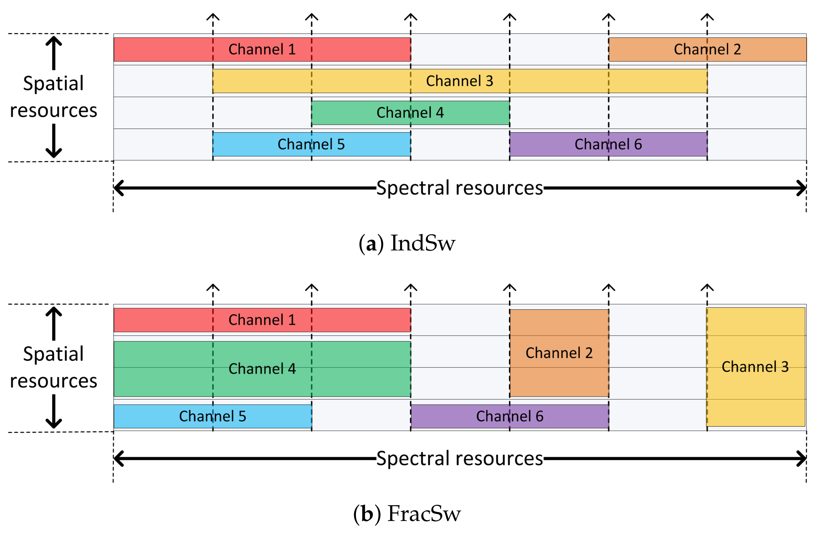In this paper we put our attention on the SMFB due to its support for the largest range of the switching policies, including (i) independent switching (IndSw)—each spatial mode can be freely directed to any output port, and (ii) fractional (or group) switching (FracSw)—spatial modes can be switched in groups containing a subset of all modes [2,3,4]. The selected switching policy determines the structure of possible communication channels. IndSw allows only for the allocation using the spectral channels (SChs) where each SCh groups a number of adjacent slices allocated on the exactly one spatial mode (see Figure 1a). IndSw brings the best spectrum utilization, however, at the cost of a high switching complexity [2]. FracSw on the contrary supports additionally the spectral-spatial channels (SSChs) where each SSCh involves a number of slices allocated on a number (subset) of spatial modes (see Figure 1b). In turn, FracSw brings a significantly lower switching complexity and a lower spectrum efficiency compared to IndSw.

The problem of allocating demands in SS-FONs is called routing, space and spectrum allocation (RSSA). It was proved to be more challenging than corresponding problems in WDM or EON networks without the spatial multiplexing [2]. RSSA aims at assigning each traffic demand with a light-path, which is defined as a connection of a routing path (connecting demand end nodes) and a channel allocated on the path links. As mentioned before, the channel can be either spectral or spatial-spectral depending on the applied switching policy.

Concurrently, the telecommunication networks have become an indispensable part of the society every-day life, providing support for a vast range of human activities—business, education, health care, finances, entertainment, social life, etc. As a result, their continuous and uninterrupted operation is required and provided by means of either protection or restoration methods [5]. The restoration process, which is in the focus of that paper, is run after a failure occurs. It aims at the restoring as much traffic as possible (i.e., re-allocating demands whose paths are no longer available) with respect to the current network resource availability. Due to the existence of additional spatial dimension, SS-FON solution brings new possibilities for the efficient flow restoration. In more detail, an SSCh is usually narrower in the spectrum domain than an SCh accommodating the same bit-rate. Hence, FracSw may be more efficient than IndSw in specific cases such as a demands’ allocation/re-allocation during high network load [6] and a flow restoration.

In this paper, we focus on the efficient modeling and optimization of the flow restoration in SS-FONs. Based on the analysis of SS-FON features, we state and verify the hypothesis that FracSw policy may be more efficient in the flow restoration task than the IndSw. To this end, we study a two-phase optimization problem, which consists of: (i) the network planning with respect to the spectrum usage and (ii) the flow restoration after a single link failure aiming at maximizing the restored bit-rate. Both related subproblems we formulate using the integer linear programming (ILP) approach applied with two flow modeling techniques—the node-link (ND) and the link-path (LP). Based on the extensive numerical experiments, we compare the proposed models and specify the range of their applicability. Next, we use them to study the efficient flow restoration in SS-FON realized using SMFB. In the investigation, we verify whether the spectral-spatial allocation may improve the flow restoration in SS-FON (compared to the restoration with only spectral channels) and we also determine the cost (i.e., the required amount of additional spectrum resources) of the full traffic restoration.

The paper is organized as follows. Section 2 reviews related works. Then, Section 3 describes the optimization tasks and provides their ILP formulations. Next, Section 4 presents the simulation results while Section 5 concludes the paper.

2. Related Works

As a promising technology for the optical transport networks, SS-FON was widely studied in the literature [2], wherein two most commonly addressed issues are SDM physical realization and related RSSA problem [2].

SDM technology brings various realization options, which were discussed in [3,7] with a special focus on their advantages, drawbacks and areas of applicability. The options include: single-mode fiber bundle (SMFB), multi-core fiber (MCF), few-mode fiber (FMF), and few-mode multi-core fiber (FM-MCF). Next, papers [3,4] elaborate SS-FON switching policies (including IndSw and FracSw) taking into account their complexity and efficiency. Eventually, manuscripts [8,9,10,11] study the crosstalk impairment in MCF-based SS-FONs and its impact on the quality of a transmission.

Concurrently, due to the high problem complexity, the research related to RSSA focuses mostly on the proposal of dedicated solution methods. They include mathematical models based on ILP technique [8,10,12,13], heuristic [8,14,15,16] and metaheuristic [8] algorithms. ILP models are primarily applied for a static network planning problem while heuristic and metaheuristic approaches are used for both—static [8,14] and dynamic [15,16] scenarios. The proposed models are mainly based on the link-path modeling technique and its extension—the candidate paths approach [8,10,17,18]. The formulations implementing the node-link modeling are applied significantly less often due to their high complexity [12]. Both modelling techniques make use of either channel-based [8,17] or slice-based [10] spectrum provisioning methods. The most commonly used optimization objective in ILP formulations is the spectrum usage [8,13,14]. The less popular definitions include for instance a combination of a spectrum usage and a network cost [17] or a resource consumption and an accepted traffic ratio [12]. It is worth-mentioning, that the above-mentioned papers only propose ILP models and do not study in detail their complexity comparing to the other modeling approaches.

Considering the survivable SS-FONs, the majority of related works focuses on the proposal of the flow protection methods based on the dedicated path protection [14,16,19], the shared backup path protection [12,14,20] or the p-cycles [21,22]. Manuscripts [12,14,19] study a static network planning problem which is modeled using ILP approach. Refs. [14,19] apply the total spectrum usage as an optimization criterion while Ref. [12] uses a combination of the number of accepted traffic (with respect to the existing crosstalks) and the spectrum usage. Then, papers related to the dynamic traffic scenarios mainly focus on the minimization of the bandwidth blocking probability by proposing dedicated heuristic algorithms. The most commonly studied failure scenario is a single link failure while only [22] takes into account a protection against a double failure. To the best of the authors’ knowledge, only Ref. [23] covers the problem of a flow restoration in SS-FONs. It focuses on its challenges with respect to the single-fiber optical technologies and the technical realization from the software define networking (SDN) controller point of view.

Summarizing, the research related to SS-FONs lacks an analysis and a comparison of various modeling approaches especially concerning node-link models. It is also deficient in studies focused on the efficient flow restoration in terms of its modeling and performance analysis. Thus, the proposed paper fills the literature gaps and covers the problem of the flow restoration in SS-FONs taking its account its modeling and efficiency.

3. ILP Models

The investigation covers a two-step optimization task: (i) the network planning, (ii) the flow restoration after a single link failure. The aim of the first step is to allocate a given set of traffic demands and minimize the total spectrum usage (i.e., the spectrum width required in the network to realize all demands). In turn, we use IndSw policy, which was proved to be the most spectrally-efficient [2]. The second step is run after a single link failure occurs. It determines the demands, which are subject to the restoration (since their working paths selected in the network planning phase are no longer available) and then tries to re-allocate them with respect to the current network resource status. Formally, the objective function in the restoration task is defined as the restored bit-rate and it should be maximized. The flow restoration process can use IndSw or FracSw policy, since the latter one is expected to improve the process performance.

Both optimization tasks are defined by ILP models using two approaches—the node-link (ND) and the link-path (LP). Please note that for the purpose of the flow restoration we need to know the demands’ working allocation rules. Regardless of the approach used in the restoration task, the working rules can be provided by either ND or LP network planning model.

We work under the assumption that the optical channels are multiplexed in a flexible grid with a standard slice width of 12.5 GHz. An elastic transceiver operates at 28 Gbaud with an optical channel bandwidth of 37.5 GHz (i.e., three frequency slices) [24] and can use one of the four modulation formats: BPSK, QPSK, 8-QAM, 16-QAM.

Table 1. Supported bit-rate and transmission distance for a transponder operating within 37.5 GHz spectrum.

	BPSK	QPSK	8-QAM	16-QAM
supported bit-rate [Gbps]	50	100	150	200
transmission reach [km]	6300	3500	1200	600

reports the supported bit-rate and the maximum transmission distance for each modulation [25]. In order to minimize the spectrum usage, we always apply the most spectrally-efficient modulation format, which satisfies the selected path length.

3.1. Network Planning Problem

SS-FON is modeled as a directed graph $G=(V,E,K)$ where V is a set of network nodes, E is a set of directed physical links and K is a set of spatial modes available on each physical link. For each network link $e\in E$, we are given a constant $l_e$, which denotes its length (in kilometers). The spectrum resources on each physical link are divided into frequency slices $s\in S$. Based on the available spectral (slices) and spatial (modes) resources, a set of channels $c\in C$ is created. Since for the network design we consider IndSw switching policy, the set C contains only SChs. Each SCh groups a number of adjacent slices located on exactly one spatial mode.

A set of static traffic demands $d\in D$ is given. Each demand, denoted by a source node $s_d$, destination node $t_d$ and bit-rate $b_d$ (in Gbps), has to be realized by means of a light-path. Each light-path consists of a routing path, which leads from the demand source node to the destination, and a channel allocated on the path links.

3.1.1. Node Link (ND) Model

In ND models, the number of slices required for a demand on a candidate routing path is not given in advance (since it depends on the path length and the applied modulation format) and therefore its calculation is incorporated into the optimization task.

Four modulation formats $m\in M$ are available (i.e., 16-QAM, 8-QAM, QPSK, BPSK), wherein $m=1$ denotes the most spectrally efficient format (16-QAM) and $m=4$ refers to the least efficient one (BPSK). Based on the model reported in Table 1, we calculate two sets of constants: (i) $a_m,m\in M$ as a lower bound of the distance range supported by the modulation m, (ii) $n_{dm},d\in D,m\in M$ as a number of slices required to realize the demand d using the modulation m. Note that $a_0=0$ km, $a_1=601$ km, $a_2=1201$ km and $a_3=3501$ km. To obtain $n_{dm}$ values for a particular demand, we compare its volume with the bit-rates supported by each of the modulation formats. For instance, having a demand d with bit-rate $b_d=120$ Gbps, it is $n_{d0}=3$ (one transponder occupying three slices), $n_{d1}=3$ (1 transponder occupying three slices), $n_{d2}=6$ (two transponders, each occupying three slices) and $n_{d3}=9$ (three transponders, each occupying three slices). Then, we define a set of constants $h_{dm}$ indicating the number of slices required to realize the demand d using the modulation format m instead of the m−1. Please note that $h_{d1}=n_{d1}$ and $h_{dm}=n_{dm}-n_{d(m-1)},m>1,m\in M$.

ND model of the network planning is given by the objective (1) and the constraints (2)–(9). The formulation uses the following sets of variables: $x_{dec}$, $w_{dc}$, $x_{de}$, $x_d$, $u_{dm}$, $y_{eks}$ and $y_s$.

ND approach: sets and indices
$v\in V$	network nodes
$e\in E$	network physical links available in a normal state
$s\in S$	frequency slices available on each spatial mode in a normal network state
$k\in K$	spatial modes
$d\in D$	traffic demands to be realized
$c\in C$	candidate channels for the set of slices S
$m\in M$	available modulation formats
ND approach: constants
$b_d$	bit-rate (in Gbps) of the demand d
$s_d$	source node of the demand d
$t_d$	termination (destination) node of the demand d
$l_e$	length (in kilometers) of the physical link e
$a_m$	lower bound of the distance range supported by the modulation format m
$n_{dm}$	number of slices required to realize the demand d using the modulation m
$h_{dm}$	number of additional slices required for the demand d if the modulation m is applied instead of the modulation m $-1$
L	large number
$A\left(v\right)$	set of links that originate in the node v
$B\left(v\right)$	set of links that terminate in the node v
${\alpha }_{cks}$	=1, if the channel c uses the slice s on the spatial mode k; 0, otherwise
${\beta }_c$	size (the number of the involved slices) of the channel c (excluding a guard-band)
ND approach: variables
$y_{eks}$	=1, if the slice s is used on the spatial mode k and the physical link e; 0, otherwise (binary)
$y_s$	=1, if slice the s is used in the network (on any link and spatial mode); 0, otherwise (binary)
$w_{dc}$	=1, if the demand d is realized using the channel c; 0, otherwise (binary)
$x_{dec}$	=1, if the light-path selected for the demand d uses the link e and the channel c; 0, otherwise (binary)
$x_{de}$	=1, if the light- path selected for the demand d uses the link e; 0, otherwise (binary)
$x_d$	length (in kilometers) of the light-path selected for the demand d (integer)
$u_{dm}$	=1, if any modulation format $i\le m$ can be applied for the demand d; 0, otherwise (binary)

objective

$$min\sum _{s\in S}{y}_s.$$

(1)

subject to

$$\begin{array}{c}\hfill \sum _{e\in A\left(v\right)}{x}_{dec}-\sum _{e\in B\left(v\right)}{x}_{dec}=\left\{\begin{array}{cc}{w}_{dc}\hfill & \mathrm{if}v=s_d\hfill \\ -w_{dc}\hfill & \mathrm{if}v=t_d\hfill \\ 0\hfill & \mathrm{if}v\ne s_d,t_d\hfill \end{array}\right.\\ \hfill d\in D,c\in C,v\in V.\end{array}$$

(2)

$$\sum _{c\in C}{w}_{dc}=1,d\in D.$$

(3)

$$\sum _{e\in E}{l}_e·x_{de}\le x_d,d\in D.$$

(4)

$$\sum _{c\in C}{x}_{dec}=x_{de},d\in D,e\in E.$$

(5)

$$x_d-a_m\le L·u_{dm},d\in D,m\in M.$$

(6)

$$\sum _{m\in M}{u}_{dm}·h_{dm}\le \sum _{c\in C}{w}_{dc}·{\beta }_c,d\in D.$$

(7)

$$\sum _{d\in D}\sum _{c\in C}{x}_{dec}·{\alpha }_{cks}=y_{eks},e\in E,k\in K,s\in S.$$

(8)

$$y_{eks}\le y_s,e\in E,k\in K,s\in S.$$

(9)

The objective function (1) defines the total spectrum usage. Equation (2) is the flow conservation constraint. Then, Formula (3) guarantees that the exactly one channel is chosen for each demand while Formula (4) calculates the length of a routing path selected for each demand. Next, Equation (5) defines the variable $x_{de}$, which informs if the link e belongs to the routing path selected for the demand d. Formula (6) selects a modulation format for each traffic demand while (7) guarantees that the size of a selected channel for a demand is greater or equal to the number of slices required for that demand. Eventually, Equations (8) and (9) determine the variables $y_{eks}$ and $y_s$, which control the spectrum usage and non-overlapping.

3.1.2. Link-Path (LP) Model

For the purpose of LP models, we assume that the n different routing paths are available for each pair of network nodes. The paths are generated off-line by means of Yen’s kSP algorithm with respect to the links’ physical lengths (in kilometers) and taking into account only links, which have not been affected by a failure. Hence, there are n different candidate routing paths $p\in P_d$ for each traffic demand $d\in D$.

Then, for each demand $d\in D$ we generate a set of its candidate light-paths $l=(p,c)\in L_d$ based on the candidate routing paths $p\in P_d$ and the channels $c\in C$. Note that for each demand d and its candidate path p (with a given length), we apply the most spectrally-efficient modulation format, which satisfies the path length. For that modulation, we obtain the required channel width and only channels of that size are used to create the candidate light-paths. Hence, in the case of LP models the modulation selection and the channels size calculation tasks are solved off-line and are not included in the optimization tasks.

LP model of the network planning is given by the objective function (10) and the constraints (11)–(13). The formulation uses the following sets of variables: $y_{eks}$, $y_s$ and $z_{dl}$.

LP model: sets and indices
$e\in E$	network physical links available in a normal state
$s\in S$	frequency slices available on each link in a normal network state
$k\in K$	spatial modes
$d\in D$	traffic demands to be realized
$c\in C$	candidate channels for the set of slices S
$p\in P_d$	candidate routing paths for the demand d considering all network links E
$l=(p,c)\in L_d$	candidate light-paths for the demand d considering the set of links E and the set of channels C
LP model: constants
n	number of routing paths available for each pair of network nodes
${\alpha }_{cks}$	=1, if the channel c uses the slice s on the spatial mode k; 0, otherwise
${\gamma }_{le}$	=1, if the light-path l uses the link e; 0, otherwise
LP model: variables
$y_{eks}$	=1, if the slice s is used on the spatial mode k and the physical link e; 0, otherwise (binary)
$y_s$	=1, if the slice s is used in the network (on any link and spatial mode); 0, otherwise (binary)
$z_{dl}$	=1, if the demand d is realized using the light-path l; 0, otherwise (binary)

objective

$$min\sum _{s\in S}{y}_s.$$

(10)

subject to

$$\sum _{l\in L_d}{z}_{dl}=1,d\in D.$$

(11)

$$\sum _{d\in D}\sum _{l\in L_d}{z}_{dl}·{\gamma }_{le}·{\alpha }_{c\left(l\right)ks}=y_{eks},e\in E,k\in K,s\in S.$$

(12)

$$y_{eks}\le y_s,e\in E,k\in K,s\in S.$$

(13)

The objective (10) defines the total spectrum usage (similarly like (1)). The Equation (11) selects exactly one light-path for each demand. The last two formulas, i.e., (12) and (13), determine the variables $y_{eks}$ and $y_s$ that control the spectrum usage and non-overlapping. Note that the Equation (13) is also a part of node-link model (Equation (9)).

3.2. Flow Restoration Problem

The flow restoration task is performed after a single link failure occurs. Therefore, we consider here a modified network topology $G^{\prime }=(V,E^{\prime },K)$. We assume that one physical link is broken and no longer available for a transmission. Hence, the set of available links is decreased by the broken link, i.e., $e\in E^{\prime }\in E$. What is more, we work under the assumption that there might be additional spectrum resources available for the purpose of the restoration. Thus, the set of available slices is $s\in S^{\prime },|S^{\prime }|=\rho ·|S|$ where $\rho \ge 1$ is a constant indicating the ratio of the additional resources and $\left|S\right|$ is the spectrum width required to allocate all demands in the network planning phase. Note that $\rho =1$ means that no additional resources are available for the restoration. We are also given the network resource availability due to the realization of the failure unaffected demands. Let the binary constant ${\gamma }_{eks}$ indicates if the slice s is allocated on the spatial mode k on the physical link e. Based on the currently available slices $s\in S^{\prime }$, the set of restoration channels $c\in C^{\prime }$ is calculated. The channels can be either spectral or spatial-spectral since both IndSw and FracSw are available in the restoration task. Each SSCh allocates a number of adjacent slices on $K_c$ spatial modes wherein the same slices are reserved on all modes. Note that $K_c=1$ means that only SChs are allowed (i.e., IndSw). Eventually, we are given a set of demands to be restored, i.e., the demands whose working paths are no longer available due to the failure – $d\in D^{\prime }\in D$. The aim of the restoration task is to re-allocate as much bit-rate as possible with respect to the network resource availability.

3.2.1. Node-Link (ND) Model

ND model of the flow restoration is given by the objective function (14) and the constraints (15)–(21). The formulation uses the following sets of variables: $x_{dec}$, $w_{dc}$, $x_{de}$, $x_d$, $u_{dm}$, $y_{eks}$ and $r_d$.

ND approach: sets and indices (additional)
$e\in E^{\prime }$	network physical links available after a single link failure
$s\in S^{\prime }$	frequency slices available on each spatial mode during a restoration process. Note that $|S^{\prime }|=\rho ·|S|$
$d\in D^{\prime }$	traffic demands to be restored
$c\in C^{\prime }$	candidate channels for the set of slices $S^{\prime }$
ND approach: constants (additional)
$\rho$	ratio of the additional spectrum resources available for the purpose of flow restoration
${\delta }_{eks}$	considering a particular network state:
	=1, if currently the slice s is occupied on the spatial mode k on the physical link e; 0, otherwise
ND approach: variables (additional)
$r_d$	=1, if the demand d is released due to a failure; 0, otherwise (binary)

objective

$$max\sum _{d\in D^{\prime }}(1-r_d)·b_d$$

(14)

subject to

$$\sum _{c\in C^{\prime }}{w}_{dc}+r_d=1,d\in D^{\prime }.$$

(15)

$$\begin{array}{c}\hfill \sum _{e\in A\left(v\right)}{x}_{dec}-\sum _{e\in B\left(v\right)}{x}_{dec}=\left\{\begin{array}{cc}{w}_{dc}\hfill & \mathrm{if}v=s_d\hfill \\ -w_{dc}\hfill & \mathrm{if}v=t_d\hfill \\ 0\hfill & \mathrm{if}v\ne s_d,t_d\hfill \end{array}\right.\\ \hfill d\in D^{\prime },c\in C^{\prime },v\in V.\end{array}$$

(16)

$$\sum _{e\in E^{\prime }}{l}_e·x_{de}\le x_d,d\in D^{\prime }.$$

(17)

$$\sum _{c\in C^{\prime }}{x}_{dec}=x_{de},d\in D^{\prime },e\in E^{\prime }.$$

(18)

$$x_d-a_m\le L·u_{dm},d\in D^{\prime },m\in M.$$

(19)

$$\sum _{m\in M}{u}_{dm}·h_{dm}\le \sum _{c\in C^{\prime }}{w}_{dc}·{\beta }_c,d\in D^{\prime }.$$

(20)

$$\sum _{d\in D^{\prime }}\sum _{c\in C^{\prime }}{x}_{dec}·{\alpha }_{cks}+{\delta }_{eks}=y_{eks},e\in E^{\prime },k\in K,s\in S^{\prime }.$$

(21)

The objective function (14) defines the total restored bit-rate after a failure. Formula (15) assures that each demand is either realized (i.e., has assigned exactly one channel) or is released. Eventually, Equation (21) controls the spectrum usage and non-overlapping. Comparing to (8), Formula (21) takes into account the current resource availability (denoted by ${\delta }_{eks}$) and the allocation of the demands subject to the restoration. The rest of constraints is analogue to these from the network planning phase, however, they are defined for the modified network topology and the set of demands.

3.2.2. Link-Path (LP) Model

For the purpose of the flow restoration, we calculate n different routing paths for each pair of network nodes considering the modified network topology $G^{\prime }$. Then, using these paths and the candidate channels $c\in C^{\prime }$, we calculate the candidate restoration light-paths $l\in L_d^{\prime }$ for the demands subject to the restoration $d\in D^{\prime }$.

LP model of the flow restoration problem is given by the objective (22) and the constraints (23), (24). The formulation uses the following sets of variables: $y_{eks}$, $z_{dl}$ and $r_d$.

LP model: sets and indices (additional)
$e\in E^{\prime }$	network physical links available after a single link failure
$s\in S^{\prime }$	frequency slices available on each spatial mode during a restoration process. Note that $|S^{\prime }|=\rho ·|S|$
$d\in D^{\prime }$	traffic demands to be restored
$c\in C^{\prime }$	candidate channels for the set of slices $S^{\prime }$
$p\in P_d^{\prime }$	candidate routing paths for the demand d considering the set $E^{\prime }$ of available links
$l=(p,c)\in L_d^{\prime }$	candidate light-paths for the demand d considering the set of links $E^{\prime }$ and the set of channels $C^{\prime }$
LP model: constants (additional)
$\rho$	ratio of the additional spectrum resources available for the purpose of flow restoration
${\delta }_{eks}$	considering a particular network state:
	=1, if currently the slice s is occupied on the spatial mode k on the physical link e; 0, otherwise
LP model: variables (additional)
$r_d$	=1, if the demand d is released due to a failure; 0, otherwise (binary)

objective

$$max\sum _{d\in D^{\prime }}(1-r_d)·b_d$$

(22)

subject to

$$\sum _{l\in L_d^{\prime }}{z}_{dl}+r_d=1,d\in D^{\prime }.$$

(23)

$$\sum _{d\in D^{\prime }}\sum _{l\in L_d^{\prime }}{z}_{dl}·{\gamma }_{le}·{\alpha }_{c\left(l\right)ks}+{\delta }_{eks}=y_{eks},e\in E^{\prime },k\in K,s\in S^{\prime }.$$

(24)

Equation (23) instead of (11) says that each demand is either realized (i.e., has assigned exactly one light-path) or is released. Next, Formula (24) controls the spectrum usage and non-overlapping. Comparing to (12), Equation (24) takes into account the current resource availability (denoted by ${\delta }_{eks}$) and the allocation of other demands that are subject to the restoration.

3.3. Complexity Analysis

The computational complexity of an ILP model is determined mostly by the number of included constraints and variables.

Table 2. Complexity of the proposed ILP models: the number of constraints and variables as a function of the problem characteristics.

	Number of Constraints	Number of Variables
network planning problem
ND model	$2\left|E\right|\left|K\right|\left|S\right|+\left|D\right|(3+|E|+|M|+|C\left|\right|V\left|\right)$	$\left|S\right|\left(\right|E\left|\right|K|+1)+\left|D\right|(1+|M|+|E|+|C|+|C\left|\right|E\left|\right)$
LP model	$\left|D\right|+2\left|E\right|\left|K\right|\left|S\right|$	${\sum }_{d\in D}|L_d|+|S\left|\right(\left|E\right|\left|K\right|+1)$
flow restoration problem
ND model	$|E^{\prime }\left|\right|K\left|\right|S^{\prime }|+|D^{\prime }\left|\right(3+|E^{\prime }|+|M|+|C^{\prime }\left|\right|V\left|\right)$	$|E^{\prime }\left|\right|K\left|\right|S^{\prime }|+|D^{\prime }\left|\right(2+|C^{\prime }|+|M|+|E^{\prime }|+|E^{\prime }\left|\right|C^{\prime }\left|\right)$
LP model	$|D^{\prime }|+|E^{\prime }\left|\right|K\left|\right|S^{\prime }|$	$|D^{\prime }|+{\sum }_{d\in D^{\prime }}|L_d^{\prime }|+|E^{\prime }\left|\right|K\left|\right|S^{\prime }|$

analyses the complexity of the proposed models as a function of the problem characteristics. Let us focus firstly on the network planning problem. The complexity of ND model is mainly affected by the number of traffic demands $\left|D\right|$ and the candidate channels $\left|C\right|$. The number of channels is in turn determined by the number of spatial models $\left|K\right|$ and the available spectrum width $\left|S\right|$ (i.e., $\left|C\right|=f\left(\right|K|,|S|$). Depending on the testing scenarios, the model can include more constraints or variables. LP model on the contrary involves relatively low number of constraints (determined by the number of demands $\left|D\right|$, links $\left|E\right|$, spatial $\left|K\right|$ and spectral $\left|S\right|$ resources) and its complexity is mostly imposed by the number of included variables. The number of variables depends mainly on the number of demands $\left|D\right|$ and the candidate light-paths for each demand $|L_d|$. The number of candidate light-paths is not the same for all demands but generally it is a function of the number of candidate paths for each pair of nodes—n, the spectrum width $\left|S\right|$ and the number of spatial resources $\left|K\right|$, i.e., $|L_d|=f(n,\left|S\right|,\left|K\right|)$. The models’ complexity for the flow restoration problem are described by similar formulas as for the network planning, however, the problem is considered in the modified topology. It means that: (i) one network link is broken, (ii) only a subset of demands subjects to the restoration, (iii) some network resources are reserved for the failure unaffected demands, (iv) if FracSw is allowed the number of channels and light-paths is also determined by the parameter $K_c$.

Based on the data in the Table 2 we can conclude that the complexity of LP model is significantly lower than the complexity of ND model when LP is applied with a low number of candidate paths, spectral and spatial resources. While the values of these parameters increase, the complexity of LP approach exceeds the complexity of ND model.

In order to control spectrum provisioning, the proposed models define and use the channel structures. Each channel is characterized by the first slice index, number of involved slices and index(es) of assigned spatial mode(s). It is also possible to use a slice-based approach to control the spectrum usage in ILP models. In this method, the special sets of variables are created for each demand indicating indexes of: (i) the first allocated slice, (ii) the last allocated slice, (iii) the assigned spatial mode (or the group of spatial modes). The complexity of slice-based models is in turn mostly determined by the number traffic demands. The comparison of the channel-based and slice-based approaches applied for SS-FON optimization was performed in [13]. It revealed that the first of them is more suitable for large demands’ sets while the latter performs better when a high number of spectral/spatial resources is available. It is also worth-mentioning that the channel-based method allows us to precisely control which channels are taken into account (for instance if the channels are spectral or spectral-spatial) and therefore it was applied in this paper.

4. Results and Discussion

The results of simulations are divided into two parts. The first one focused on the comparison of the node-link and the path-link models for the problems of the network planning and the flow restoration. The main goal of that part was to determine the most suitable models for further simulations. The second part of the investigation was a case study which evaluated the potential benefits of the spectral-spatial allocation in the flow restoration process as well as determining the cost of full restoration (i.e., the amount of additional spectrum resources that were required to restore 100% of the initial traffic) in SS-FON.

We used two realistic network topologies, i.e., PL12 and DT14, which modeled the Polish and German national network, respectively. The topologies are presented in Figure 2 and characterized in

Table 3. Characteristics of the examined topologies.

	PL12	DT14
number of nodes	12	14
number of links	36	46
avg nodal degree	2.9	3.3
min link length [km]	70	37
max link length [km]	360	353
avg link length [km]	185	182

. For each topology we considered different overall traffic volume (selected to provide reasonable processing times) and for each volume we defined 10 different sets of unicast demands. In all sets, the demand end nodes and bit-rate were generated uniformly at random wherein their bit-rates came from the range 10–500 Gbps.

For the purpose of experiments, ILP models were implemented in Visual Studio 2017 integrated with IBM CPLEX 20.1.0 by means of C++ programming language. The simulations were conducted using IBM Flex System computing cluster available in the Department of Systems and Computer Networks, Wroclaw University of Science and Technology (https://www.kssk.pwr.edu.pl/) (accessed on 1 May 2021). It was equipped with two Intel Xenon 8C E5-26902 processors, two 128 GB SSD, HDD hard drives and 256 GB DDR-1600 of RAM memory. To provide fair and repeatable computing environment, each program instance (solving ILP model) was assigned with a separate processor thread and could use up to 16 GB of RAM memory.

All presented results are averaged over 10 different sets of demands. Due to the limited space of the paper, we present results only for the selected configurations, which reveal important trends and observations.

4.1. Models Comparison

The models were compared separately for two optimization tasks—the network planning and the flow restoration.

4.1.1. Network Planning Problem

We studied SS-FON realized using SMFB with $\left|K\right|\in \{1,2,3,4\}$ spatial modes and the overall traffic volume equal to 2.0, 2.5, ..., 4.5 Tbps. For LP model we assume that $n\in \{5,10,15,20,25,30\}$ different routing paths are given for each pair of the network nodes and we denote it as LP(n).

Table 4. Comparison of the node-link and the link-path models for the network planning problem and PL12—the average gap to global optimum [%] and the processing time [s] (for each $\left|K\right|$ value and traffic volume, the best result is bold).

Traffic	$\left|\mathit{K}\right|=2$							$\left|\mathit{K}\right|=3$
[Tbps]	ND	LP(5)	LP(10)	LP(15)	LP(20)	LP(25)	LP(30)	ND	LP(5)	LP(10)	LP(15)	LP(20)	LP(25)	LP(30)
gap to global optimum
2.0	0.00%	0.48%	0.48%	0.00%	0.00%	0.00%	0.00%	0.00%	0.00%	0.00%	0.00%	0.00%	0.00%	0.00%
2.5	0.00%	4.70%	3.75%	3.75%	3.75%	2.50%	1.25%	0.00%	0.00%	0.00%	0.00%	0.00%	0.00%	0.00%
3.0	0.00%	4.23%	0.00%	0.00%	0.00%	0.00%	0.00%	0.00%	1.43%	0.00%	0.00%	0.00%	0.00%	0.00%
3.5	0.00%	6.25%	3.75%	3.75%	3.75%	3.75%	2.50%	0.00%	0.48%	0.00%	0.00%	0.00%	0.00%	0.00%
4.0	0.00%	5.36%	0.00%	0.00%	0.00%	0.00%	0.00%	0.00%	0.00%	0.00%	0.00%	0.00%	0.00%	0.00%
4.5	0.00%	10.23%	6.48%	6.48%	6.48%	6.48%	0.00%	0.00%	0.00%	0.00%	0.00%	0.00%	0.00%	0.00%
processing time [s]
2.0	5490.2	0.61	0.92	1.39	2.10	2.49	3.06	11,331.94	0.76	1.29	2.23	2.96	3.50	3.84
2.5	16,898.9	0.61	0.89	1.25	1.76	3.90	7.70	17,485.22	0.55	0.72	0.91	1.09	1.80	3.73
3.0	31,939.4	2.13	4.20	9.75	11.89	12.47	14.10	24,378.62	1.87	2.57	3.49	4.05	4.23	5.14
3.5	47,150.3	2.73	7.61	17.62	20.08	22.25	25.46	30,960.82	1.67	2.96	4.07	4.72	5.01	6.01
4.0	125,781.8	9.70	21.13	32.14	30.66	35.05	52.03	100,357.6	3.38	3.94	5.23	9.79	13.35	13.31
4.5	313,770.7	13.01	25.82	40.00	45.11	53.61	77.40	446,313.9	6.06	8.80	11.89	19.41	20.19	33.57

compares ND and LP(n) models for PL12 in terms of a gap to the optimal solution (i.e., the difference between the obtained and the optimal result divided by the optimal result) and the processing time. The results for DT14 followed the same trends. By the definition ND model always provided optimal solutions but at the cost of a long processing time (in the considered experiments—up to several days for a single demands set). LP model on the contrary did not guarantee globally optimal solutions and the quality of its results strongly depended on the applied n value. However, it terminated significantly faster (in the considered experiments—up to several minutes for a single demands set) compared to ND model. For further experiments with network planning problem we strongly recommend LP(n = 30) since it provided suboptimal results and a short processing time.

4.1.2. Flow Restoration Problem

For the flow restoration problem, we considered SS-FON realized using SMFB with the $\left|K\right|=7$ spatial modes and the overall traffic volume equal to 5, 10, ..., 25 Tbps. For each of the defined demand sets, we used LP(n = 30) model to allocate demands in the network (and minimize the spectrum usage). Next we simulated a single link failure, determined the set of demands which require a restoration and then used ND or PL model to restore as much traffic as possible. Note that in all cases only a fraction of initial traffic was subject to the restoration and therefore we considered larger traffic volumes in that part of experiments. To compare ND and LP models for the flow restoration task, we used two criteria: the ratio of the restored traffic (the restored bit-rate divided by the total bit-rate that was subject to the restoration) and the processing time. To create the restoration light-paths, we assumed LP(n = 30) and $K_c\in \{1,2,3,4\}$. Note that $K_c=1$ indicated that only spectral channels were allowed (i.e., IndSw policy). The candidate paths in LP restoration model were generated with respect to the current network state (i.e., working links and available spectrum resources). For each demand set we subsequently simulated failure of each network link $e\in E$ and then presented the final results averaged over $\left|E\right|$ links and 10 demands sets.

Table 5. Comparison of the node-link and the link-path models for the traffic restoration problem for $\rho =1.0$: the average ratio of the restored traffic [%] and the processing time [s] (for each topology and traffic volume, the best result is bold).

	PL12 Topology						DT14 Topology
Traffic	Node-Link Model			Link-Path Model			Node-Link Model			Link-Path Model
[Tbps]	${\mathit{K}}_{\mathit{C}}=\mathbf{1}$	${\mathit{K}}_{\mathit{C}}=\mathbf{2}$	${\mathit{K}}_{\mathit{C}}=\mathbf{3}$	${\mathit{K}}_{\mathit{C}}=\mathbf{1}$	${\mathit{K}}_{\mathit{C}}=\mathbf{2}$	${\mathit{K}}_{\mathit{C}}=\mathbf{3}$	${\mathit{K}}_{\mathit{C}}=\mathbf{1}$	${\mathit{K}}_{\mathit{C}}=\mathbf{2}$	${\mathit{K}}_{\mathit{C}}=\mathbf{3}$	${\mathit{K}}_{\mathit{C}}=\mathbf{1}$	${\mathit{K}}_{\mathit{C}}=\mathbf{2}$	${\mathit{K}}_{\mathit{C}}=\mathbf{3}$
ratio of restored traffic [%]
5T	99.1%	100.0%	100.0%	97.1%	97.1%	97.1%	97.9%	100.0%	100.0%	96.0%	96.0%	96.0%
10T	100.0%	100.0%	100.0%	97.1%	97.1%	97.1%	94.8%	98.3%	98.5%	86.6%	86.6%	86.6%
15T	97.3%	97.6%	97.8%	76.4%	76.4%	76.4%	90.4%	93.3%	93.3%	65.3%	65.3%	65.3%
20T	94.9%	95.3%	95.4%	48.0%	48.0%	48.0%	83.7%	86.1%	86.7%	37.6%	37.6%	37.6%
25T	92.1%	93.0%	93.3%	28.0%	28.0%	28.0%	82.4%	84.6%	85.1%	31.9%	31.9%	31.9%
processing time [s]
5T	3.31	6.87	21.46	33.79	34.49	33.44	3.73	9.29	31.95	27.21	44.91	42.77
10T	6.06	17.13	29.27	51.65	51.04	48.24	9.76	22.07	49.94	33.18	54.13	51.90
15T	13.89	24.98	38.25	52.98	51.67	48.85	11.02	21.00	31.29	27.34	46.03	45.39
20T	13.15	18.47	24.58	38.86	38.66	37.85	10.04	17.09	27.47	41.25	42.47	38.59
25T	9.70	6.98	20.81	29.79	29.33	29.19	10.56	21.62	45.60	34.14	35.26	32.98

and

Table 6. Comparison of the node-link and the link-path models for the traffic restoration problem for $\rho =1.4$: the average ratio of the restored traffic [%] and the processing time [s] (for each topology and traffic volume, the best result is bold).

	PL12 Topology						DT14 Topology
Traffic	Node-Link Model			Link-Path Model			Node-Link Model			Link-Path Model
[Tbps]	${\mathit{K}}_{\mathit{C}}=\mathbf{1}$	${\mathit{K}}_{\mathit{C}}=\mathbf{2}$	${\mathit{K}}_{\mathit{C}}=\mathbf{3}$	${\mathit{K}}_{\mathit{C}}=\mathbf{1}$	${\mathit{K}}_{\mathit{C}}=\mathbf{2}$	${\mathit{K}}_{\mathit{C}}=\mathbf{3}$	${\mathit{K}}_{\mathit{C}}=\mathbf{1}$	${\mathit{K}}_{\mathit{C}}=\mathbf{2}$	${\mathit{K}}_{\mathit{C}}=\mathbf{3}$	${\mathit{K}}_{\mathit{C}}=\mathbf{1}$	${\mathit{K}}_{\mathit{C}}=\mathbf{2}$	${\mathit{K}}_{\mathit{C}}=\mathbf{3}$
ratio of restored traffic [%]
5T	100.0%	100.0%	100.0%	100.0%	100.0%	100.0%	100.0%	100.0%	100.0%	100.0%	100.0%	100.0%
10T	100.0%	100.0%	100.0%	99.9%	99.9%	99.9%	99.4%	99.6%	100.0%	96.7%	96.7%	96.7%
15T	99.5%	100.0%	100.0%	95.0%	95.0%	95.0%	98.9%	99.4%	99.9%	88.2%	88.2%	88.2%
20T	98.4%	99.8%	99.9%	84.4%	84.4%	84.4%	97.6%	99.4%	100.0%	75.0%	75.0%	75.0%
25T	96.0%	97.3%	99.3%	59.0%	59.0%	59.0%	95.2%	97.5%	99.3%	62.9%	62.9%	62.9%
processing time [s]
5T	8.70	23.98	172.86	73.47	73.42	73.27	8.79	21.12	219.47	92.15	91.72	91.80
10T	19.13	88.98	127.84	112.11	112.26	112.17	24.03	63.88	328.26	126.14	126.82	128.52
15T	43.34	94.17	150.27	150.94	150.54	151.40	29.82	67.50	228.65	113.69	112.92	112.62
20T	42.24	105.74	226.65	130.23	130.54	130.61	24.22	59.87	96.93	122.93	122.90	122.95
25T	31.12	96.15	346.50	107.32	107.63	107.56	30.50	61.35	203.84	98.89	99.41	98.99

compare ND and PL models in the flow restoration task for, respectively, $\rho =1.0$ and $\rho =1.4$. For all studied cases for $K_c=4$ the ratio of restored traffic was 100%. We do not present these values, to make the tables more readable. First of all, we observed important relationship between the restoration complexity and the overall traffic volume in the network. The higher overall bit-rate was, the more traffic was affected by a single failure. Therefore, the results showed a decreasing efficiency of the restoration process with the increasing traffic volume. For all considered cases, we observed that ND model significantly outperformed LP model in terms of the ratio of the restored traffic. Its efficiency reached at least 82.4% for $\rho =1.0$ and at least 95.2% for $\rho =1.4$. LP model on the contrary restored at least 28% of traffic for $\rho =1.0$ and at least 59% of traffic for $\rho =1.4$. Moreover, in the case of ND model we could observe the benefits of the spectral-spatial allocation (i.e., the implementation of $K_c>1$). For instance, the application of $K_c=3$ instead of $K_c=1$ allowed us to restore up to 4% more of the traffic for DT14 and 25T. The processing time for $\rho =1.0$ was from several up to several dozen seconds for a single test case regardless of the model. For $\rho =1.4$ the calculations took up to several minutes. Regardless of the applied $\rho$ value, the processing time of ND model remarkably increased with $K_c$ value. The same dependence was not observed for the second approach. For the considered scenarios, the times of calculations were acceptable for both models. Moreover, we observed that for many cases the processing time of LP formulation was longer than the processing time of ND one. The high complexity of LP model followed from the enormous set of the candidate light-paths, which could be created using n = 30 routing paths and all possible channels (especially when the spectral-spatial channels were allowed).

Due to its high efficiency and acceptable processing time, we strongly recommend applying ND model for further experiments with the flow restoration task.

4.2. Efficient Flow Restoration in SS-FON—Case Study

In the last part of experiments, we focused on the efficient flow restoration in SS-FONs realized using SMFB. We analyzed potential benefits of the spatial-spectral allocation in the restoration task and the amount of additional spectrum resources that were required for the full traffic restoration.

Similarly to Section 4.1.2, we studied a two-stage problem. In the first stage, we solved the network planning problem considering the allocation of 5, 10, ..., 25 Tbps volume of randomly generated unicast demands. For each traffic volume, we generated 10 different sets of demands. Then, we allocated these sets using LP(n = 30) model and saved the obtained allocation rules and the required spectrum width. Next, we moved to the flow restoration stage. For each defined demands set, we subsequently simulated a failure of link $e\in E$ and use ND model to perform the traffic restoration assuming the available spectrum width to be $\rho =1.0,1.1,...,2.0$ times higher than the width obtained in the network planning phase. In the experiments we set $\left|K\right|=7$ and $K_c\in \{1,2,3,4\}$. The results are presented in Figure 3, Figure 4, Figure 5, Figure 6, Figure 7 and Figure 8 for PL12 and DT14, accordingly. 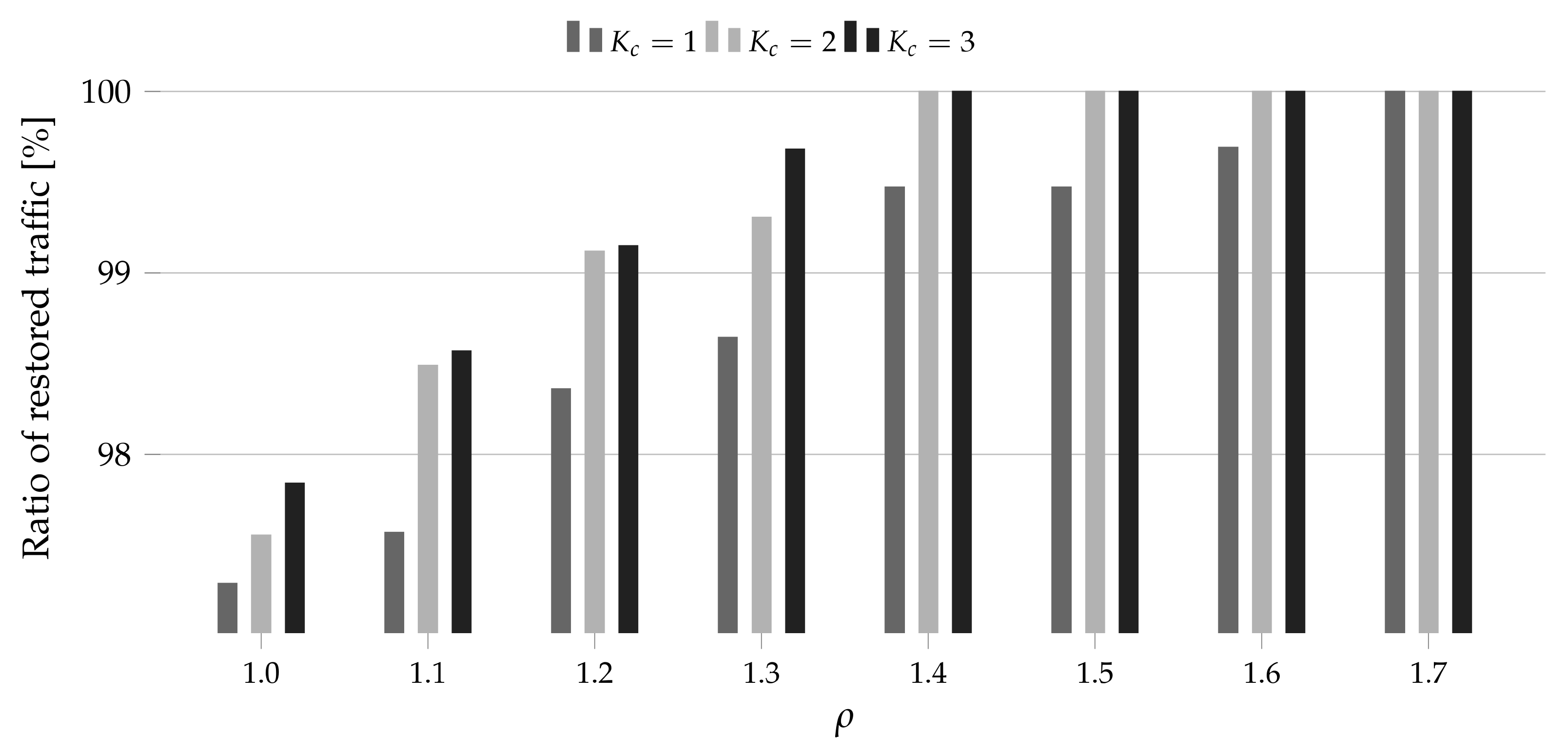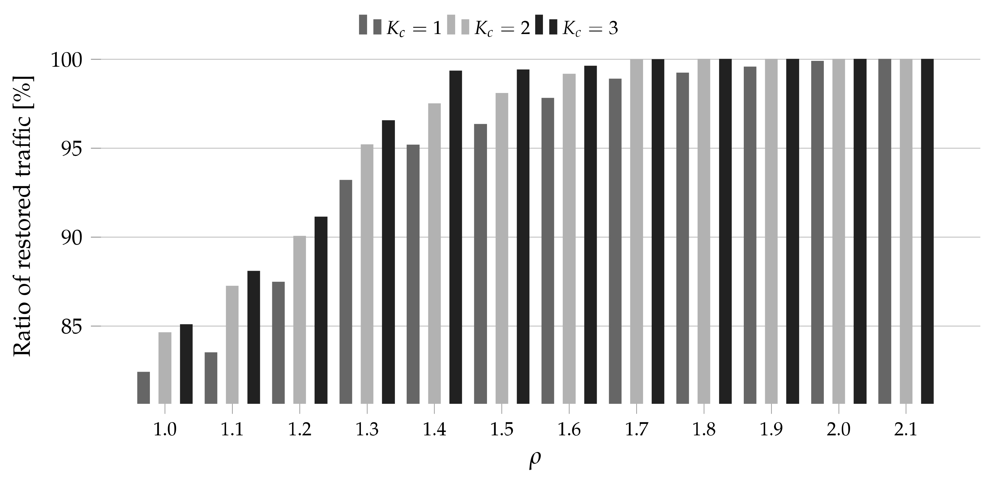For $K_c=4$ it was possible to restore 100% of traffic for all studied cases. In order to increase the figures readability, we did not include these results.

Note that the analysis of the ratio of restored traffic as a function of $\rho$ allowed us to determine the cost of the full traffic restoration—the lowest value of $\rho$ for which the ratio of restored traffic was equal to 100%. For instance, if the full traffic restoration was observed for $\rho =1.1$, then the cost was equal to 10% (since 10% more spectrum resources are required (compared to the spectrum width obtained in the network planning phase) to restore the whole traffic).

In all considered cases, we observed that the spectral-spatial restoration ($K_c\ge 1$) brought a higher efficiency than the only spectral restoration ($K_c=1$). In the considered study, the spectral-spatial restoration allowed us to restore up to 4.75% more traffic (DT14, 15T, $\rho =1.2$). Therefore, the findings proved the initial thesis stating that the spectral-spatial allocation may improve the restoration process in SS-FONs. Next, let us focus on the cost of the full traffic restoration. According to the results, the cost increased with the overall traffic volume in the network (and in turn the volume of the traffic subjects to the restoration) and was higher for the larger network topology. Moreover, the application of the spectral-spatial allocation allowed us to reduce that cost. For instance, for both topologies and 5 Tbps, we needed 30% more spectrum (compared to the spectrum required for allocation in the the failure-free network state) to restore the whole traffic when only the spectral allocation was available. For the same case, we did not need any additional resources when the spectral-spatial allocation was allowed. For PL12 and 15 Tbps, we needed 70% more spectrum to restore the whole required bit-rate using the spectral channels while only 40% more resources were required when the spectral-spatial channels could be applied (for the same traffic volume the corresponding values for DT14 were 90% and 60%). Eventually, for DT14 and 25 Tbps, we needed 110% more spectrum for the spectral full restoration versus 80% for the spectral-spatial full restoration. Therefore, we observed that the cost of full traffic restoration depended on plenty of factors (wherein the most important were the initial traffic volume and the topology size) while the application of the spectral-spatial allocation could reduce its value about 30%.

5. Conclusions

In this paper, we focused on the efficient modeling and the optimization of the flow restoration in SS-FONs realized using SMFB. For that purpose, we defined a two-step optimization task consisting of: (i) the network planning aiming at minimizing the spectrum usage, (ii) the flow restoration after a single link failure targeting at maximizing the restored bit-rate. Both subproblems we defined using ILP technique combined with the node-link and the link-path modelling approaches. Then, we performed the extensive numerical experiments divided into two parts: (i) the comparison of proposed optimization approaches and the selection of most suitable ones, (ii) the efficient flow restoration in the SS-FONs case study. The goals of the case study were to verify whether the spectral-spatial allocation may improve the restoration efficiency in SS-FONs compared to the restoration with only the spectral channels and to determine the cost of the full traffic restoration (the amount of additional spectrum resources required to restore the whole bit-rate). The results of the simulations show that the spectral-spatial allocation allows us to restore up to 4% more traffic compared to the restoration with only spectral channels. They also reveal that the cost of the full traffic restoration depends on plenty of factors, including the overall traffic volume in the network and the network size, while the spectral-spatial allocation allows us to reduce its value about 30%.

In the future work, we plan to further develop tools for an efficient flow restoration in SS-FON. In more detail, we plan to design some dedicated heuristic methods to address calculations in extremely large networks.