Abstract
The preservation of relevant mutual information under compression is the fundamental challenge of the information bottleneck method. It has many applications in machine learning and in communications. The recent literature describes successful applications of this concept in quantized detection and channel decoding schemes. The focal idea is to build receiver algorithms intended to preserve the maximum possible amount of relevant information, despite very coarse quantization. The existent literature shows that the resulting quantized receiver algorithms can achieve performance very close to that of conventional high-precision systems. Moreover, all demanding signal processing operations get replaced with lookup operations in the considered system design. In this paper, we develop the idea of maximizing the preserved relevant information in communication receivers further by considering parametrized systems. Such systems can help overcome the need of lookup tables in cases where their huge sizes make them impractical. We propose to apply genetic algorithms which are inspired from the natural evolution of the species for the problem of parameter optimization. We exemplarily investigate receiver-sided channel output quantization and demodulation to illustrate the notable performance and the flexibility of the proposed concept.
1. Introduction
The information bottleneck method is a powerful framework from the machine learning field [1]. Its fundamental idea is to compress an observed random variable to some compressed representation according to a compression rule. This rule is designed to preserve so-called relevant mutual information I, where is a properly chosen relevant random variable of interest. The method is very generic and has numerous applications, for example, in image and speech processing, in astronomy and in neuroscience [2,3,4].
In the past few years, the method has also attracted considerable attention in the communications community. It was revealed to be useful in the design of strongly quantized baseband signal processing algorithms for detection and channel decoding with low complexity, but performance close to that of non-quantized conventional reference algorithms [5,6,7]. The communications-related applications of the method lead from the design of channel output quantizers over the decoding of low-density parity-check codes and polar codes to entire baseband receiver chains that include channel estimation and detection [5,6,7,8,9,10,11,12,13]. Fundamentally, the idea of most aforementioned applications of the method in communications is to design deterministic compression mappings that replace the classical arithmetical operations in the baseband signal processing algorithms. These mappings are typically considered as lookup tables that store the respective t for each possible y. The lookup table approach sketched above is well-suited for many of the baseband signal processing problems already studied in communications. In some other applications, however, it is desirable to have an arithmetical rule or a sequence of processing steps in an algorithm which maps an observed realization y onto the compressed t. This is the case, for example, when the cardinality of and, therefore, the resulting lookup table implementing becomes fairly large. As a result, it is meaningful to consider parametrized compression mappings with M parameters that preserve a desired large amount of mutual information I.
In this article, we develop parametrized mappings for communication receivers that only need few parameters and simple signal processing operations to preserve significant amounts of relevant information. The mappings investigated use exact or approximate nearest neighbor search algorithms [14,15]. Other approaches to designing parametrized systems exist in the literature. Some of the most popular use neural networks [16,17,18]. Our motivation to study the proposed nearest neighbor search-based systems instead is that they offer a very simple implementation with a small number of mathematical operations to determine the system output t. This is an important aspect for their practical use in communication receivers.
Finding optimum parameters , however, is cumbersome for the proposed parametrized mappings, especially if approximate nearest neighbor search algorithms are used. Therefore, we use genetic algorithms for the required optimization of the parameters . Genetic algorithms are very generic and powerful optimization algorithms that are inspired by the natural evolution of the species [19,20]. Their general idea is to create a population of candidate solutions to an optimization problem. Then, a so-called fitness of each individual in the population is evaluated with respect to the target function. The members of the population breed novel generations by combining their genetic information using simple crossover operators. In this process, the Darwinistic principle of promoting solutions with higher fitness is applied and also mutations happen. Fascinatingly, like this genetic algorithms can in fact find very good solutions to very complicated optimization tasks [19,20,21,22].
The above motivates us to apply genetic algorithms to optimize parametrized compression mappings that aim for maximum preservation of relevant information. Such mappings have numerous applications in learning and also in the baseband signal processing of communication receivers. This article investigates the receiver-sided channel output quantization in communication receivers based on nearest neighbor search algorithms, similar to the original conference version of this article [23]. As novel contributions, we introduce and optimize parametrized mappings that involve K-dimensional trees [24,25]. We propose and investigate the design of a novel demodulation scheme for data transmission using non-binary low-density parity-check codes with binary phase-shift keying (BPSK) modulation which is based on nearest neighbor search in the K-dimensional trees as an entirely new contribution of this article.
In summary, the contributions of this article are:
- We develop and investigate the idea of applying genetic algorithms to maximize mutual information in a parametrized information bottleneck setup for communication receivers.
- We design very powerful parametrized compression mappings that preserve large amounts of relevant information with very few parameters. These mappings are based on exact and approximate nearest neighbor search algorithms.
- We illustrate enormous flexibility and generality of the considered approach.
- We present results on channel output quantization and demodulation in communication receivers.
The article is structured as follows. The next section provides a brief overview of the required preliminaries. In Section 3, we propose different classes of parametrized mappings that can preserve significant amounts of relevant information. Moreover, we motivate and explain their genetic optimization. Section 4 then provides practical results on the proposed communication receiver design with maximum preservation of relevant information. Finally, Section 5 concludes the article.
2. Preliminaries
This section introduces fundamentals on the information bottleneck method and genetic algorithms. At the end of the section, two important distance metrics for vectors are briefly recalled that will be required in the remainder of the article.
2.1. The Information Bottleneck Method
The information bottleneck method is an information theoretical framework introduced by N. Tishby et al. in [1]. It originates from machine learning and considers three discrete random variables and which form a Markov chain . is termed the relevant random variable. The idea is that is observed and shall be compressed to a more compact representation . It is well-known from the famous rate-distortion theory that in this context a compression corresponds to minimizing the so-called compression information I. However, it shall be guaranteed that also the mutual information I is maximized. As a result, one can conclude that defines which features of are considered to be relevant and shall be preserved under compression. The compression rule that maps a realization onto its compressed representation is typically considered as a conditional probability distribution . This allows us to cover probabilistic and also deterministic mappings of y onto t. In this article, however, we will restrict ourselves to deterministic mappings that, of course, fulfill the law of total probability. In this situation, t is a determinstic function of y, i.e., .
There exist many information bottleneck algorithms [26,27,28,29,30] that can construct the desired compression mapping for a given cardinality of . A popular information bottleneck algorithm in communications is the KL-means algorithm from [26,27]. Due to the fact that is discrete, it is possible to store the mapping in a lookup table with size by just storing each t for the respective y. The mapping then clusters the event space of into several clusters which, mathematically, are the preimages of .
2.2. Genetic Algorithms
Genetic algorithms are very powerful and generic optimization algorithms that have various applications in many fields of engineering [19,20,21,22]. They aim to mimic the natural evolution of the species to solve multi-parameter optimization problems. Consider the problem of finding parameters that maximize a function .
In order to find optimum parameters , a genetic algorithm works on a population of candidate solutions. Initially, this population is often drawn randomly. The real world parameter description is typically termed the phenotype of an individual in the population. Each member of the population implies a certain value of the target function which is readily termed the fitness of this individual.
In addition to the phenotype description of every individual, a genotype description can be introduced. The idea is to encode the numerical values of the parameters using so-called alleles into a long genetic string. In the simplest form, the alleles are just binary zeros or ones and the genotype of an individual is a long sequence of these numbers, accordingly. For a given phenotype, one can determine the genotype by considering uniform discretization of the search spaces for the parameters into regions, respectively. Like this the values of the parameters can be interpreted as bit sequences of length which encode the corresponding index of the region in binary form. A simple method to obtain the respective bit sequences is determining the region indices for all the appearing in as
The are integers and can be converted into their binary representations easily. Then, one just concatenates all the obtained binary numbers to a long binary string to obtain the genotype. As an example, consider , . One obtains , and the corresponding genotype . Of course, the reverse genotype to phenotype conversion can be done similarly.
An instance of the population exists in a generation of the genetic algorithm. In every generation, parent solutions are randomly selected from and their genetic information is combined using simple genetic crossover operators on the genotypes to create children which form the population of the following generation. Such a crossover operation with crossover positions is illustrated in Figure 1.
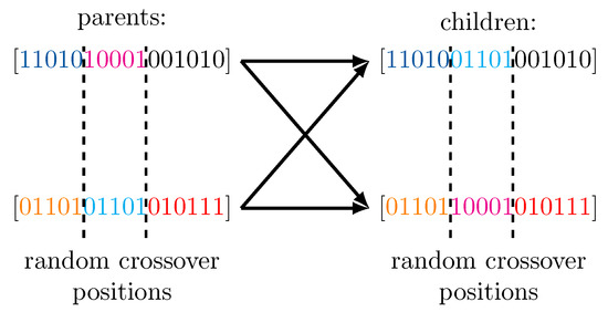
Figure 1.
Illustration of a two point crossover in the processing of a genetic algorithm. The genotypes of the children are formed by combining the genotypes of both parents.
It is key that in the described processing, the individuals with higher fitness are more likely to become parents of the next generation than the weaker individuals with lower fitness. This is realized using simple inversion sampling to draw the parents. Moreover, the concept of elitism promotes the fittest individuals and guarantees them propagating their genetic material into the next generation. Finally, mutations of alleles in the genotypes of the children are performed with a certain mutation probability to assure some diversity.
Fascinatingly, when the processing is executed for several generations, genetic algorithms can find very good solutions to enormously complicated optimization tasks [19]. A particular strength of genetic algorithms is their generality. They need no other assumptions on the target function than that it allows to measure the fitness of an individual in the population. This motivates us to investigate the possibility of maximizing the preserved relevant information I under compression in information bottleneck settings with genetic algorithms.
2.3. Distance Metrics
In this section, we want to briefly recall two elementary distance metrics for vectors and that will be used frequently in the remainder of the article. A well-known distance measure is the Euclidean distance between and , i.e.,
When it comes to implementation, the Euclidean distance has some disadvantages. In particular, taking the square under the root in Equation (2) requires costly multiplications in digital hardware. In addition, the square root is also costly on some signal processing platforms. As a result, in some applications a more favorable distance is the Manhattan distance [31] given by
This distance measure only requires sign inversions and additions which are fairly low-cost operations.
3. Design of Parametrized Compression Mappings That Maximize Relevant Information for Communication Receivers
The general system setup that we consider in this article is sketched in Figure 2.
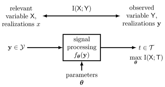
Figure 2.
Optimizing parameters in a parametrized information bottleneck like setup. The parameters shall be tuned to maximize for a given parametrized function .
As shown there, we consider a generic receiver-sided signal processing scheme that inputs an observed random variable . The observed random variable is a random vector with realizations because many signal processing components in communications process more than one scalar input variable. The system has M tunable parameters , . The design idea for tuning the parameters is choosing them, such that the mutual information is maximized. Like this, the system output shares a desired huge amount of information with the relevant random variable . We consider the system output to be from some finite set with cardinality . Only this cardinality , the mapping rule of onto t implied by and the joint probability distribution determine . In contrast, does not depend on the particular elements of . The reason is that is determined only by the probability distributions , and , as this mutual information is given by
After all, the considered system design can be understood as an instance of the information bottleneck method described in Section 2.1. In contrast to the classical information bottleneck approach from [1], however, a parametrized system design for the mapping of realizations onto t by is considered here. In addition, the choice of the output cardinality allows us to adjust an inherent compression level achieved by the system, as this cardinality determines the number of bits required to represent the system output.
The system design approach introduced in Figure 2 has very intuitive applications in the communications context. Consider, for example, the data transmission scheme sketched in Figure 3. In this example, a phase shift keying (PSK) modulation scheme is used to transmit data over a complex additive white Gaussian noise (AWGN) channel. The transmission of the complex symbol yields the channel observation at the receiving end. Obviously, the system fed with the samples in vector notation should preserve information on the transmitted modulation symbol x in this example. Considering outputs to be from a discrete set of integers , the system conducts a q bit quantization of the continuous received samples y with a minimum loss of relevant information on the transmitted modulation symbol x. In addition, each implies a conditional probability distribution . Therefore, the considered system can also be used straightforwardly for demodulation of the transmitted symbol x. The considered system will be investigated further in Section 4.
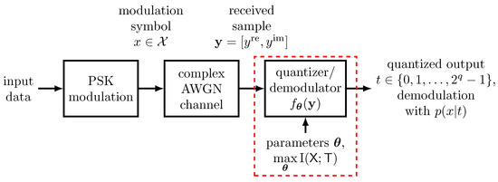
Figure 3.
Exemplary application of a parametrized mapping for the quantization and demodulation of an AWGN channel output under PSK modulation. The system output shall be highly informative about the transmitted modulation symbol .
3.1. Flexible Parametrized Mappings
Independent of the techniques used for the parameter optimization that we will describe later, the system design sketched above needs flexible classes of parametrized functions which allow to preserve significant amounts of relevant information for properly tuned parameters . We propose different ideas to implement the mapping of onto in the considered systems which are described in the following. The considered mappings are all instances of nearest neighbor search algorithms [14] which need the definition of a distance metric like the ones from Section 2.3.
3.1.1. Clustering by Simple Exact Nearest Neighbor Search
The first class of parametrized mappings of onto that we consider determines the outgoing t for an incoming as
where is some properly defined, but at the same time, arbitrary distance measure between an incoming vector and an optimized parameter vector of the same dimension N as . In this article, we will consider the Euclidean distance and the Manhattan distance from Section 2.3, but we want to stress that the proposed method can deal with arbitrary distances. This mapping is characterized by such parameter vectors which we compactly gather in a long vector . As each vector has length N, there are parameters in . Clearly, the approach is very much inspired by a vector quantizer which we aim to design with a genetic algorithm such that it maximizes the mutual information I.
In its simplest form, the considered mapping can be implemented by calculating all possible distances and choosing the vector with the smallest distance. This approach is sometimes also termed the naive nearest neighbor search [14], but for small values of it offers a quite practical solution to identifying the nearest neighbor. The integer index t of the closest found vector then is the output of the system.
3.1.2. Exact and Approximate Nearest Neighbor Clustering Using K-Dimensional Trees
The simple nearest neighbor search approach from above has the apparent disadvantage that its complexity grows linearly with . As a result, the simple nearest neighbor search is limited to moderate cardinalities in practice. Aiming for , however, often requires quite large cardinalities .
Fortunately, so-called K-dimensional tree data structures [24,25] can help to reduce the complexity of the simple nearest neighbor search algorithm for large . These data structures can often determine the nearest neighbor of without explicitly calculating all possible distances . The resulting average query complexity of a K-dimensional tree scales logarithmically with the number of vectors , hence typically resulting in a drastic reduction of required distance calculations in comparison to the simple nearest neighbor search. It shall be mentioned, however, that the worst case complexity of a search still is . K denotes the dimensionality of the data. In our case, K corresponds to the number N of inputs processed by the system from Figure 2.
Figure 4 shows an exemplary K-dimensional tree which can be used to conduct nearest neighbor search in an exemplary set of vectors with length that we have chosen randomly for illustration purposes. We consider the task of finding the node with the smallest Euclidean distance to an exemplary query vector that is also provided in Figure 4. The true nearest neighbor of is with Euclidean distance .
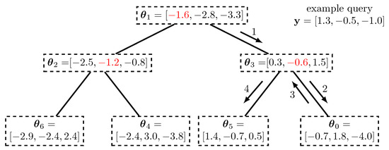
Figure 4.
Exemplary K-dimensional tree with length random vectors . The vectors are arranged according to decision thresholds given by the axis coordinate highlighted in red in the subsequent levels of the tree. Arrows indicate the processing of querying the nearest neighbor of the vector .
The general principle of the search in the K-dimensional tree is that most of the explicit distance calculations are avoided and replaced by very simple threshold decisions along the axis of the data points. As it is highlighted in red in Figure 4 in the root node, the first axis considered corresponds to the first coordinate . It is easy to see that all points in the left half of the tree underneath the root node fulfill and all the points in the right half have .
As a result, for querying the first coordinate of is compared with the first coordinate of the root node. Due to the fact that , the query goes to the right child of the root node which is indicated using the arrow labeled 1. This processing is now repeated, but in the next reached node, the axis to split is the second, i.e., , as indicated in red again. The change of the considered axis in the subsequent levels of the tree is fundamental. In each level, only the distances to the visited nodes are calculated and only their minimum is stored and tracked. At node we have the distance in our example.
Obviously, the example query follows the path labeled 2, as and the query reaches the leaf node . The distance to this node is , so stays closer.
The described processing does not guarantee finding the true nearest neighbor of which is given by so far. Fascinatingly, however, it is very easy to find out, whether the decision for a certain axis made so far went into the direction of the true nearest neighbor. In order to do that, backtracing the path taken is required. In each visited node now the distance of along the split axis of the data in that node has to be considered only. If this distance is smaller, than the minimum distance obtained so far, it follows that following the other branch could be better.
In our example, when is visited again, it is easy to find that the distance along axis in the node is , so the other branch labeled by arrow 4 is taken into account and the true nearest neighbor is found. The backtracing now can reach the root node and the processing is over.
Interestingly, the described processing can be implemented very elegantly using the programming method of recursion. The recursion for the backtracing, however also adds a significant amount of complexity. It is, therefore, mentionable that a very simple approximate nearest neighbor search algorithm with much lower complexity can be implemented in the K-dimensional tree by dismissing the backtracing. Like this, the search complexity can be fixed to . The results presented in Section 4.2 show that in the considered application no practically relevant disadvantage of using approximate instead of exact nearest neighbor search exists.
Exactly as in Section 3.1.1, the (approximate) nearest neighbor seach algorithm outputs the index t of the closest found point which is the system output from Figure 2.
3.1.3. Approximate Nearest Neighbor Clustering Using Neighborhood Graphs
Another reduced complexity approximate algorithm for the problem of finding an approximate nearest neighbor of a query point exists in the literature [14,15]. This algorithm is based on a proximity neighborhood graph of nodes that correspond to the candidate points . For simplicity, we consider neighborhood graphs, where all nodes have neighbors which correspond to the closest points under the considered distance.
The neighborhood graph-based approximate nearest neighbor search algorithm is depicted in Figure 5. When a new query point shall be located, one enters the graph from any entry node and checks whether or not there are points in the neighborhood of the entry node which are closer to the query than the entry node itself. If this is the case, the closest found neighbor becomes the novel entry node and the processing starts over. In the shown example, the processing will stop after the neighbors of the entry node have been processed. Of course, this procedure can be executed for several initial entry nodes to improve the accuracy. It is also very easy to add a complexity constraint on the maximum number of allowed distance calculations by only allowing a certain path length while jumping through the neighborhood graph. In order to achieve a desired minimum of distance calculations in the design, we define a set of entry nodes and first choose to determine the closest entry node to the query from that set. Then we only run the approximate nearest neighbor search described above from the closest found entry node. In the considered design, the worst case number of distance calculations to determine t for a given is given by
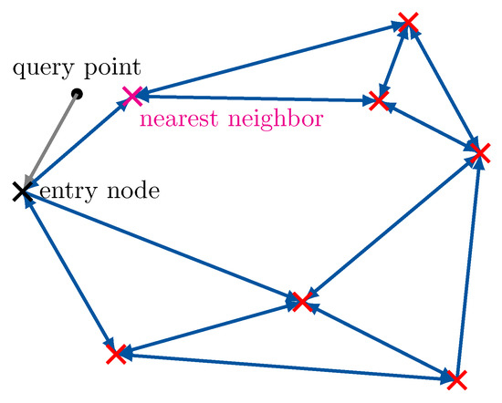
Figure 5.
Visualization of the approximate nearest neighbor search in a neighborhood graph. The algorithm traverses through the neighborhood graph greedily. × markers correspond to the parameters to be optimized, blue arrows indicate neighborhood relations.
Please note that this number is independent of . As a result, one can allow for a very large number of candidate vectors without a proportional increase in the number of required distance calculations.
Again the approximate nearest neighbor search algorithm then just outputs the integer index t of the approximate closest point to . Clearly, the possible performance of the algorithm in terms of the preservation of I and its complexity depend on the parameters , and especially on which defines the sparsity of the neighborhood graph. Moreover, the particular set of entry nodes has an impact on the preserved relevant information. We will see in the practical results in Section 4, that quite sparse graphs with few entry nodes and small path length have the ability to preserve very significant amounts of I.
3.2. Genetic Algorithm Optimization
In Section 3.1.1, Section 3.1.2 and Section 3.1.3, different approaches to the problem of finding the (approximate) nearest neighbor of the system input from Figure 2 were proposed and described. Our intention is using the described approaches to implement the mapping . In doing so, the parameters shall be tuned, such that the mutual information is maximized for a given . This naturally raises the question of how we can determine optimum parameters . We propose to perform the optimization of the parameters for the considered mappings and irrespective of the used distance function with a genetic algorithm for various reasons explained in the following. Afterwards, we describe how to perform the parameter optimization with a genetic algorithm.
3.2.1. Why Genetic Algorithms?
Standard parameter optimization problems are often tackled by the application of gradient-based methods. A very famous example for this is the parameter optimization required to train neural networks in machine learning [16].
Considering Equation (5) again, however, reveals that using a gradient-based approach is cumbersome in our context. This equation involves a min operation which causes differentiability issues. A typical way to overcome them would be to use a smooth approximation [31], e.g., the softmin operation instead of the min during optimization, but we note that like this, we would in fact not optimize the deterministic mapping rule that we aim for in Equation (5), but only some non-deterministic approximation. Genetic algorithms, however, can directly optimize the deterministic mapping rule, as will be explained soon.
Moreover, depending on the distance metric used, more issues can arise. If the Manhattan distance from Equation (3) shall be used, the non-differentiability of the absolute magnitude involved adds to the min from Equation (5) which makes a gradient approach for the optimization of the parameters very cumbersome and would require mathematical approximations and workarounds [31]. Genetic algorithms, in contrast, can easily deal with this matter.
Finally and most importantly, in Section 3.1.2 and Section 3.1.3, we have also studied approximate solutions to the nearest neighbor problem. These have drastically reduced complexity in terms of the number of distance calculations required. If such heuristic algorithms are applied, one can imagine the min operation from Equation (5) to be replaced with an approximate min. This operation is extremely hard, if not impossible, to describe analytically. Considering the greedy processing of the approximate nearest neighbor search algorithms from Section 3.1.2 and Section 3.1.3, it is intuitively clear that for both, there is no mathematical expression to adequately describe the mapping of onto t, even though it is deterministic. The mapping rules are rather given by subsequent processing steps in greedy algorithms.
As a result, the parameter optimization to maximize I with standard gradient methods is not possible in these cases. Genetic algorithms, however, can be applied easily as discussed in the following.
3.2.2. Using Genetic Algorithms to Maximize the Preserved Relevant Information
We propose to perform the optimization of the parameters for all considered mappings and irrespective of the actually used distance function with a genetic algorithm. For that purpose, we initially draw a population of individuals . As it is typically assumed in the information bottleneck setup, we assume that the joint probability distribution is known.
For any population member it is then straightforward to determine the joint probability distribution for this particular individual as
and
These distributions directly allow us to calculate the respective preserved relevant information I for this population member according to Equation (4), that is,
Note that by definition. This allows us to use the mutual information directly as fitness of the population members in the generations of the genetic algorithm. The rest of the processing then just follows the standard processing of genetic algorithms using selection, genetic crossovers and mutations over the generations as described, for example, in [19,20].
It is very important to note that all the involved equations can be evaluated totally irrespective of the actual operations performed in the signal processing block from Figure 2. The presented equations in fact work for all possible deterministic mappings of onto . The genetic algorithm just treats as a black box. Therefore, we can just use either the exact or the approximate nearest neighbor search approaches from Section 3.1.1, Section 3.1.2 and Section 3.1.3. We can also freely decide what distance measure we want to use. As a result, the presented approach is very generic.
4. Results and Discussion
This section presents results on the application of the proposed parametrized compression mappings for quantizing the output of a communications channel and demodulation with the developed system design approach. It shall be mentioned that the applications studied serve to illustrate the method and the performance of the designed mappings. They allow us a very vivid illustration that reveals insights into the working of the proposed method. However, numerous other applications can be investigated in future work, for example, in channel decoding, detection and other receiver-sided baseband signal processing tasks [5,6,7,8,9,10,11,12,13].
4.1. Quantization of the Channel Output with Minimum Loss of Relevant Information
In the following, we first consider KL-means quantization as proposed in [26]. KL-means quantization shall serve as a benchmark for the designed parametrized compression mappings. The most important figure of merit that we consider is the preserved relevant information I for a given output cardinality of the designed quantizers.
4.1.1. Information Bottleneck Quantizer Design with the KL-Means Algorithm
An intuitive application of the information bottleneck method in communications is the design of a channel output quantizer that maximizes the relevant information on the transmitted modulation symbols . As already discussed and shown in Figure 3, in this context, corresponds to the received channel output. If is continuous, for example, for an AWGN channel, it has to be very finely discretized to uniformly spaced samples on some interval of interest. is the quantized output variable of the quantizer. A q bit quantizer designed with the Information Bottleneck method maps realizations y onto quantization indices , such that and I max. I is independent of the elements in . We consider integer quantization indices that need q bits in the hardware.
As in [26], we consider complex AWGN channels and complex modulation alphabets, such that the continuous received sample at a certain time instance is
where is a realization of a complex valued, circularly symmetric Gaussian process with variance and mean 0 and is a complex modulation symbol. For a simple notation, we assume that y is already finely discretized using a large number of uniformly spaced samples in a grid on the complex plane with points for and , respectively. In addition, we define the vector representation of the received sample.
In this situation, we want to quantize to a number of quantization regions. The considered quantizers are particularly useful for phase-shift keying (PSK) signals [26]. An example for 8-PSK under AWGN with noise variance is provided in Figure 6. This figure shows the quantization regions obtained with the KL-means algorithm in the complex plane.
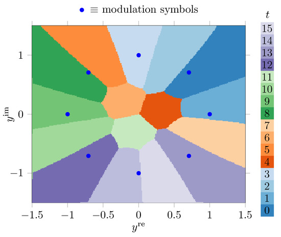
Figure 6.
Quantization regions for the output of an AWGN channel with 8-PSK modulation in the complex plane for , constructed with the KL-means algorithm. I bit, I bit.
For this example, and were both finely discretized into uniformly spaced samples on the interval with properly paying attention to clipping effects. Like this, one obtains a grid with cardinality in the complex plane. This grid was quantized to different quantization regions. This implies strong compression.
A typical application of the designed quantizer could be in a radio, where the analog-to-digital converter has a resolution of 8 bits for the real and the in-phase component of the received signal, but the signal shall be quantized to be processed further using just 4 bits per sample with minimum relevant information loss. In this example, I bit and I bit. This indicates that despite the very coarse quantization a significant amount of relevant information on the transmitted modulation symbols (that is, around ) is preserved. Hence, it illustrates that the KL-means algorithm preserves relevant information.
Note that, due to the very complicated shape of the optimized quantization regions obtained using the KL-means algorithm from Figure 6, this quantizer cannot be characterized by simple thresholds for and . The KL-means algorithm instead delivers a table which holds the respective for all of the possible vectors , such that, effectively one ends up with a lookup table of size 65,536 that characterizes the quantizer.
4.1.2. Genetic Algorithm Quantizer Design Using Exact Nearest Neighbor Search
Figure 7 shows the quantization regions obtained for a simple exact nearest neighbor search approach described in Section 3.1.1.
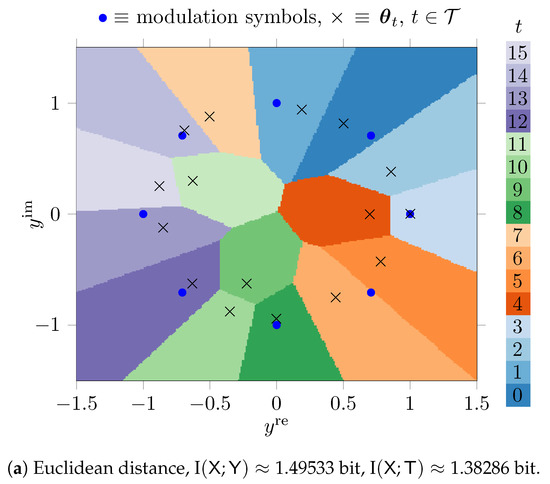
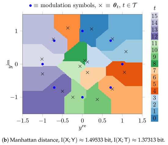
Figure 7.
Quantization regions for the output of an AWGN channel with 8-PSK modulation in the complex plane for , constructed with the genetic algorithm.
Figure 7a uses the Euclidean distance and Figure 7b uses the Manhattan distance in Equation (5). The parameters were tuned using the genetic algorithm based method from Section 3.2.2.
For the genetic algorithm optimization, we have used the configuration consolidated in Table 1. This configuration was determined experimentally and found to yield good results.

Table 1.
Overview of parameters of the genetic algorithm.
The phenotypes in this scenario hold real valued parameters that represent the real and the imaginary parts of 16 complex numbers. The optimized parameters are denoted using × markers in Figure 7 in the complex plane. As it can be seen, the genetic algorithm automatically learns favorable positions in terms of the maximum preservation of I under the respective distance . The quantizers from Figure 7a,b both can be described with parameters, but have quantization regions with very complicated shapes that allow us to preserve large amounts of relevant information. The preserved relevant mutual information is I bit (i.e., of I) for the Euclidean distance and I bit (i.e., of I) for the Manhattan distance.
The conference version of this article [23] also holds a quantitative comparison for different signal-to-noise ratios (SNRs) that we skip here for brevity.
4.1.3. Genetic Algorithm Quantizer Design with Approximate Nearest Neighbor Search
The numbers presented in the prior section illustrate that for , there is still a mentionable gap between I and I for all considered quantizers. In order to close that gap, one has to increase the output cardinality of the quantizer to further decrease the quantization loss. This, however, proportionally increases the number of distance calculations for the method from Section 3.1.1. Here we use the approximate nearest neighbor search algorithm from Section 3.1.3 to overcome that issue. Figure 8 compares the preserved relevant information I of the KL-means algorithm and the proposed genetic algorithm optimized compression mappings for an output cardinality of as a function of the SNR of the AWGN channel. Due to its simpler distance calculation, we only consider the Manhattan distance here. For this investigation, we were forced to decrease the cardinality of the grid that finely discretizes the complex plane to points for , respectively. The reason is that the time complexity of the KL-means algorithm from [26] is proportional to the product and with as used in the previous investigation and used here, it was just not possible to create the KL-means quantizers in a reasonable time, even though we have used a highly-parallel implementation of that algorithm which parallelizes the algorithm on a graphics card [32]. Please note that using a coarser grid slightly degrades I. This indicates that using the KL-means algorithm for very large cardinalities is challenging. The method proposed here, however, easily allows using such a large .
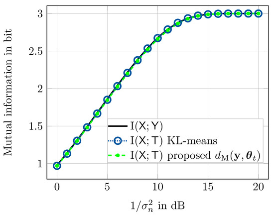
Figure 8.
Comparison of KL-means and genetic algorithm optimized quantization using approximate nearest neighbor search from Section 3.1.3 for in terms of preserved I. I serves as an ultimate upper bound.
The approximate nearest neighbor search algorithm from Section 3.1.3 used the parameters neighbors, entry nodes and a maximum path length of . These parameters were found to offer a good tradeoff between sparsity of the neighborhood graph and performance. The worst case number of distance calculations to determine t for a given in this setting is according to Equation (6) which is significantly less than . During our experiments we found out that it is even possible to reduce the maximum number of distance calculations further by decreasing or at the expense of very slight losses in I. Moreover, we have added the choice of the first entry node as a parameter to the genetic algorithm such that it is included in the optimization process. The rest of the entry nodes is chosen, such that all resulting entry nodes have possibly large distances among each other. The shown results indicate that the proposed compression mappings based on the approximate nearest neighbor search algorithm from Section 3.1.3 with parameters optimized using genetic algorithms can deal with very huge cardinalities . Such large cardinalities are required to minimize the remaining quantization loss, such that I, as it can clearly be seen in Figure 8. Moreover, the performance is virtually identical to the KL-means quantizers.
4.2. Genetic Algorithm Designed Demodulation Using K-Dimensional Trees
Next, we want to investigate an application of the proposed baseband signal processing approach illustrated in Figure 2 in a data transmission system that employs a non-binary low-density parity-check code over the Galois field with for forward error correction, but uses BPSK for signalling over an AWGN channel. A data transmission scheme similar to the one studied here was investigated for a lookup table-based information Bottleneck approach in [33]. For a deep introduction to non-binary low-density parity-check codes we kindly refer the reader to [34].
Pairing a non-binary channel code with BPSK offers a particularly interesting use case of the system illustrated in Figure 2. As it will be explained in the following, in the considered setup N received samples have to be processed for the demodulation of a symbol at the receiving end. Hence, this problem perfectly matches the architecture of the considered system.
For completeness, it shall be mentioned that it is also common to pair non-binary channel codes with -ary modulation schemes, for example, -PSK. For such a coding and modulation scheme, the demodulation problem can be conducted using the systems investigated in Section 4.1. To do so, one has to use after the quantization, as it has already been mentioned in Section 3.
The data transmission system that includes a non-binary channel code and BPSK modulation studied in this section is sketched in Figure 9.
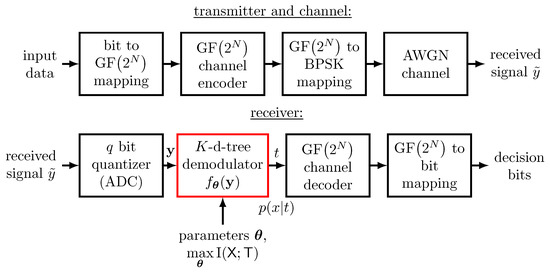
Figure 9.
Illustration of the considered data transmission scheme which employs a non-binary low-density parity-check code over GF. At the receiver, a demodulator using the nearest neighbor search from Section 3.1.2 in K-dimensional trees is employed.
The upper part of the figure shows the considered transmitter and the channel. The lower part illustrates the receiver processing including the demodulator designed with a genetic algorithm.
In the transmitter, random data bits are mapped onto GF symbols and then encoded using a non-binary low-density parity-check encoder with code rate R. In order to transmit the data over an AWGN channel using BPSK modulation, each output symbol of the encoder is mapped onto N consecutive BPSK symbols which are transmitted over the channel.
At the receiving end, first a coarse analog-to-digital conversion is performed using a q bit quantizer. N outputs from this quantizer correspond to the received samples for the transmitted BPSK symbols for a single GF output symbol of the channel encoder in this setup. The scalar channel output quantizer is designed as explained in [11].
The next crucial task of the communication receiver is to provide symbol probabilities for to the channel decoder, such that it can perform soft channel decoding. The applied channel decoder performs the iterative sum-product algorithm, also known as belief-propagation decoding, to decode the non-binary low-density parity-check code with a maximum of decoding iterations.
As a result, an output symbol of the channel encoder forms the relevant random variable for our proposed demodulator. We use a genetic algorithm optimized demodulator which conducts either approximate or exact nearest neighbor search in a K-dimensional tree. The demodulator determines the index t of the nearest neighbor as explained in Section 3.1.2 and delivers the symbol probability to the channel decoder. Please note that the distribution is obtained as a side product of the genetic algorithm optimization, as it is inherently determined to compute I (cf. Equations (7) and (8)).
After decoding, the decoded information symbols are transformed into the decision bits by reversing the transmitter-sided bit-to-symbol mapping. For brevity, we provide the parameters that characterize the data transmission scheme used in this section further in Table 2.
Table 2.
Overview of parameters of data transmission system.
We compare the bit error rate performances of the considered data transmission scheme including the proposed demodulation technique with state-of-the-art methods in a bit error rate simulation. Due to the fact that the optimum parameters depend on the channel , we have designed the proposed tree-based demodulators for different offline, stored them together with the corresponding distributions and used them in the simulation. The space complexity of storing the K-dimensional tree is linear in , i.e., . Therefore, storing the obtained demodulators for the different is technically not challenging and only needs a few kilobytes of memory. As a result, the construction costs of the tree were one-time costs that only affected the genetic algorithm optimization, but not the demodulator implementation.
We have used the same optimization settings for the genetic algorithm as in Section 4.1.2 and Section 4.1.3 (cf. Table 1). As a result, the design of the demodulators could be conducted offline, such that no on-the-fly generation was required. Conducting the genetic algorithm optimization only needed a few minutes on a standard computer.
As the toughest reference system, we consider a demodulator which has access to the continuous received samples in double floating point precision, i.e., no quantizer is involved. In this case, the a posteriori distribution is determined for each symbol in the transmitted codeword and delivered to the channel decoder for decoding. Assuming equally likely symbols , it is given by
where is a vector with the BPSK symbols transmitted over the channel for symbol and denotes the k-th element of this vector. Please note that this demodulator also requires calculating squared Euclidean distances in the argument of the exponential (one for each Galois field symbol). In addition, it needs several divisions and the evaluation of the exponential function. Especially the latter is costly in digital hardware. Our aim is to approach the performance of this non-quantized reference system with the proposed demodulation techniques as closely as possible while circumventing most of the costly signal processing operations.
For reference, we also consider a very simple demodulator. This demodulator performs a hard decision on the BPSK symbols on the channel and maps this hard decision onto the corresponding GF symbol directly. The decoder then is fed with a distribution that mimics with probability 1 for the hard decision symbol and 0 for all others. This system, of course, cannot profit from soft information from the demodulation process. We use it to illustrate the gains of using soft demodulation in the data transmission system.
Figure 10 shows bit error rate performances of the considered data transmission system over for the different applied demodulation techniques. Of course, the non-quantized soft-decision reference system (⋄-markers) has the best possible performance, as it suffers from no quantization loss at all. Comparing it to the system with hard demodulation (⊗-markers) shows that at an exemplary bit error rate of a soft demodulation gain of more than 3 dB over exists for this data transmission system with a non-binary low-density parity-check code over GF.
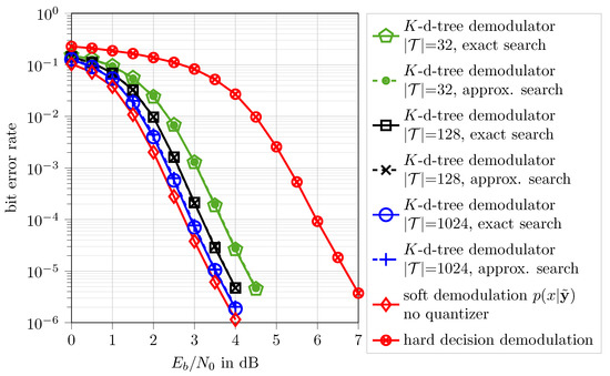
Figure 10.
Bit error rate results for non-binary GF low-density parity-check encoded data transmission over an AWGN channel with the parameters mentioned in Table 2. The proposed K-dimensional tree demodulators can achieve performance very close to the considered optimum reference system.
Interestingly, for the proposed K-dimensional tree demodulators with different cardinalities the shown results indicate that with proposed genetic algorithm optimization of the vectors , one can learn very powerful demodulators which can approach the performance of the optimum considered reference scheme up to a very slight loss over . For the demodulator with exact nearest neighbor search and (∘-markers), almost the full soft processing gain, i.e., more than 3 dB over can be realized, even though a coarse bit channel output quantizer is in place. The remaining gap to the non-quantized reference demodulator is just dB at a bit error rate of . At the same time, most of the signal processing operations inside the demodulator degenerate to simple threshold decisions along the axis of the vectors in the processing of the search in the K-dimensional tree described in Section 3.1.2. Even if the absolute number of vectors is very large, only very few distance calculations need to be performed. This goes back to the logarithmic average search complexity in the K-dimensional tree described in Section 3.1.2. As a result, using large output cardinalities like which are required to achieve performance so close to the optimum reference scheme is easily possible here. With the simple nearest neighbor search approach from Section 3.1.1, in contrast, using such a large cardinality is practically infeasible.
Another very interesting observation from Figure 10 is that the bit error rates obtained with exact and approximate nearest-neighbor search for the same output cardinalities superimpose (cf. -markers -markers, -markers). This finding is in fact very important because it highlights that the genetic algorithm automatically learns the different mapping rule applied inside the demodulator and tunes the parameters accordingly.
As it has been explained in Section 3.1.3 switching to approximate nearest neighbor search yields a fixed search complexity . In the considered case for using approximate nearest neighbor search, typically distances have to be calculated to achieve performance enormously close to the soft demodulation reference system. Please note that for a number of vectors which is a power of 2 there is the possibility that +1 distance calculations are needed. This, however only affects one of all possible paths in the tree and happens very rarely, especially if the tree is large. Therefore, the single additional distance calculation may be neglected. Anyway, we will mention it as the worst-case to be precise in the following. For the GF code used here, according to Equation (11) the soft demodulator has to determine distances to obtain the probabilities . However, it is important to note that the soft symbol demodulator reference system has a significantly higher complexity anyway.
Most importantly, the non-quantized soft demodulator uses 64 bit double floating-point values from the channel. The proposed demodulator circumvents the need of representing and processing the received samples from the channel with high precision, as it directly works on the bit output integers from the quantizer. There is no need to represent the quantized received values using real numbers as representation values, as the genetic algorithm learns to directly process the q bit quantization indices. This alone yields a significant complexity reduction of the receiver because the resolution used for the analogue-to-digital conversion of the receiver can be reduced significantly. In addition, the soft demodulator reference system requires divisions by and evaluations of the very costly exponential function in the considered case of a code. Once the right hand side of Equation (11) has been evaluated for all , one needs a normalization step to obtain a valid probability distribution which needs seven summation and eight division operations for the used GF code. All these add on top of the required eight distance calculations.
The proposed system with and approximate nearest neighbor search trades the required high precision of the analog-to-digital conversion and the numerous mentioned costly operations for typically two (worst case: three) additional distance calculations and very simple thresholding operations during the search in the K-dimensional tree. Despite this, it achieves almost identical performance as the optimum non-quantized reference scheme.
Finally, the curves for and for approximate nearest neighbor search in Figure 10 (×-markers, •-markers) reveal that even the demodulators with fewer distance calculations than the optimum soft demodulator can already realize very significant soft processing gains in comparison to the hard decision demodulator. At a bit error rate of , the demodulator with , i.e., typically just five (worst case: six) distance calculations achieves more than 2 dB soft processing gain over in comparison to the hard decision demodulator. The one for with typically seven (worst case: eight) distance calculations achieves dB and has a remaining gap of approximately dB to the non-quantized reference scheme. This illustrates that the proposed method allows to flexibly tune the trade-off between complexity and performance.
5. Conclusions
In this article, genetic algorithms were successfully applied for the optimization of parametrized compression mappings that shall preserve a maximum possible amount of relevant information. These mappings were used to build subsystems of communication receivers, i.e., channel output quantizers and demodulators. To the best of our knowledge, our conference version of this article [23] described the first application of genetic algorithms for the maximization of mutual information in this context. It investigated potential applications of this principle for distance-based channel output quantization. The results were also included in this article. The resulting distance-based quantizers can compete with quantizers designed with the KL-means information bottleneck algorithm while requiring significantly fewer parameters for their description. The graph-based approximate nearest neighbor search algorithm used in this application allows for a tunable complexity and only needs a small number of distance calculations.
As a novelty, we have developed the idea of maximizing the relevant mutual information in communication receivers with genetic algorithms further and also presented entirely new results. We have introduced the idea to apply either approximate or exact nearest neighbor search in K-dimensional trees in the receiver-sided signal processing to build signal processing blocks that aim for maximum preservation of relevant information. That technique was exemplarily used to build a novel demodulation technique for a data transmission scheme using non-binary low-density parity-check codes. The resulting demodulators can achieve the performance of a non-quantized optimum reference scheme up to a small fraction of a decibel over , even though all costly signal processing breaks down to a simple and very efficient search in a K-dimensional tree. We have also shown that using an approximate nearest neighbor search instead of an exact one does not cause significant performance degradation, but further reduces the complexity of the considered mappings based on K-dimensional trees.
The proposed method is very generic and can also be applied to other signal processing problems. A possible future application of the proposed method could be the reduced complexity decoding of non-binary low-density parity-check codes.
Author Contributions
Conceptualization, J.L., S.J.D., R.M.L.; methodology, J.L., S.J.D., R.M.L.; software, J.L., S.J.D., R.M.L.; validation, J.L., S.J.D., R.M.L.; formal analysis, J.L., S.J.D., R.M.L., M.A., M.S., P.J.; investigation, J.L., S.J.D., R.M.L., M.A., M.S., P.J.; resources, M.A.; writing—original draft preparation, J.L.; writing—review and editing, J.L., S.J.D., R.M.L., M.A., M.S., P.J.; visualization, J.L., S.J.D., R.M.L.; supervision, M.A., P.J.; project administration, M.A., M.S., P.J. All authors have read and agreed to the published version of the manuscript.
Funding
This research received no external funding.
Conflicts of Interest
The authors declare no conflict of interest.
References
- Tishby, N.; Pereira, F.C.; Bialek, W. The information bottleneck method. In Proceedings of the 37th Allerton Conference on Communication and Computation, Monticello, IL, USA, 22–24 September 1999; pp. 368–377. [Google Scholar]
- Slonim, N.; Somerville, R.; Tishby, N.; Lahav, O. Objective classification of galaxy spectra using the information bottleneck method. Mon. Not. R. Astron. Soc. 2001, 323, 270–284. [Google Scholar] [CrossRef]
- Bardera, A.; Rigau, J.; Boada, I.; Feixas, M.; Sbert, M. Image segmentation using information bottleneck method. IEEE Trans. Image Process. 2009, 18, 1601–1612. [Google Scholar] [CrossRef] [PubMed]
- Buddha, S.; So, K.; Carmena, J.; Gastpar, M. Function identification in neuron populations via information bottleneck. Entropy 2013, 15, 1587–1608. [Google Scholar] [CrossRef]
- Romero, F.J.C.; Kurkoski, B.M. LDPC decoding mappings that maximize mutual information. IEEE J. Sel. Areas Commun. 2016, 34, 2391–2401. [Google Scholar] [CrossRef]
- Lewandowsky, J.; Bauch, G.; Tschauner, M.; Oppermann, P. Design and evaluation of information bottleneck LDPC decoders for digital signal processors. IEICE Trans. Commun. 2019, E102-B, 1363–1370. [Google Scholar] [CrossRef]
- Lewandowsky, J.; Stark, M.; Bauch, G. A discrete information bottleneck receiver with iterative decision feedback channel estimation. In Proceedings of the 2018 IEEE 10th International Symposium on Turbo Codes and Iterative Information Processing (ISTC), Hong Kong, China, 25–29 November 2018. [Google Scholar]
- Hassanpour, S.; Monsees, T.; Wübben, D.; Dekorsy, A. Forward-aware information bottleneck-based vector quantization for noisy channels. IEEE Trans. Commun. 2020, 68, 7911–7926. [Google Scholar] [CrossRef]
- Kern, D.; Kühn, V. On information bottleneck graphs to design compress and forward quantizers with side information for multi-carrier transmission. In Proceedings of the 2017 IEEE International Conference on Communications (ICC), Paris, France, 21–25 May 2017. [Google Scholar]
- Steiner, S.; Kühn, V. Optimization of distributed quantizers using an alternating information bottleneck approach. In Proceedings of the 2019 23rd International ITG Workshop on Smart Antennas (WSA), Vienna, Austria, 24–26 April 2019; pp. 1–6. [Google Scholar]
- Lewandowsky, J.; Bauch, G. Information-optimum LDPC decoders based on the information bottleneck method. IEEE Access 2018, 6, 4054–4071. [Google Scholar] [CrossRef]
- Shah, S.A.A.; Stark, M.; Bauch, G. Design of quantized decoders for polar codes using the information bottleneck method. In Proceedings of the 12th International ITG Conference on Systems, Communications and Coding 2019 (SCC’2019), Rostock, Germany, 11–14 February 2019; pp. 1–6. [Google Scholar]
- Shah, S.A.A.; Stark, M.; Bauch, G. Coarsely quantized decoding and construction of polar codes using the information bottleneck method. Algorithms 2019, 12, 192. [Google Scholar] [CrossRef]
- Malkov, Y.A.; Yashunin, D.A. Efficient and robust approximate nearest neighbor search using hierarchical navigable small world graphs. IEEE Trans. Pattern Anal. Mach. Intell. 2020, 42, 824–836. [Google Scholar] [CrossRef] [PubMed]
- Prokhorenkova, L.; Shekhovtsov, A. Graph-based nearest neighbor search: From practice to theory. In Proceedings of the 37th International Conference on Machine Learning, Vienna, Austria, 12–18 July 2020; pp. 7803–7813. [Google Scholar]
- Goodfellow, I.; Bengio, Y.; Courville, A. Deep Learning; MIT Press: Cambridge, MA, USA, 2016. [Google Scholar]
- Tishby, N.; Zaslavsky, N. Deep learning and the information bottleneck principle. In Proceedings of the 2015 IEEE Information Theory Workshop (ITW), Jerusalem, Israel, 26 April–1 May 2015; pp. 1–5. [Google Scholar]
- Alemi, A.; Fischer, I.; Dillon, J.; Murphy, K. Deep variational information bottleneck. In Proceedings of the 5th International Conference on Learning Representations (ICLR) 2017, Toulon, France, 24–26 April 2017. [Google Scholar]
- Coley, D.A. An Introduction to Genetic Algorithms for Scientists and Engineers; World Scientific Publishing Co., Inc.: Singapore, 1998. [Google Scholar]
- Yu, X.; Gen, M. Introduction to Evolutionary Algorithms; Springer: London, UK, 2010. [Google Scholar]
- Elkelesh, A.; Ebada, M.; Cammerer, S.; ten Brink, S. Decoder-tailored polar code design using the genetic algorithm. IEEE Trans. Commun. 2019, 67, 4521–4534. [Google Scholar] [CrossRef]
- Wang, Y.; Li, L.; Chen, L. An advanced genetic algorithm for traveling salesman problem. In Proceedings of the 2009 Third International Conference on Genetic and Evolutionary Computing, Guilin, China, 14–17 October 2009; pp. 101–104. [Google Scholar]
- Lewandowsky, J.; Dongare, S.J.; Adrat, M.; Schrammen, M.; Jax, P. Optimizing parametrized information bottleneck compression mappings with genetic algorithms. In Proceedings of the 2020 14th International Conference on Signal Processing and Communication Systems (ICSPCS), Adelaide, Australia, 14–16 December 2020; pp. 1–8. [Google Scholar]
- Bentley, J.L. Multidimensional binary search trees used for associative searching. Commun. ACM 1975, 18, 509–517. [Google Scholar] [CrossRef]
- Brown, R.A. Building a Balanced k-d Tree in O(kn log n) Time. J. Comput. Graph. Tech. (JCGT) 2015, 4, 50–68. [Google Scholar]
- Zhang, J.A.; Kurkoski, B.M. Low-complexity quantization of discrete memoryless channels. In Proceedings of the 2016 International Symposium on Information Theory and Its Applications (ISITA), Monterey, CA, USA, 30 October–2 November 2016; pp. 448–452. [Google Scholar]
- Kurkoski, B.M. On the relationship between the KL means algorithm and the information bottleneck method. In Proceedings of the 2017 11th International ITG Conference on Systems, Communications and Coding (SCC), Hamburg, Germany, 6–9 February 2017; pp. 1–6. [Google Scholar]
- Hassanpour, S.; Wübben, D.; Dekorsy, A. A graph-based message passing approach for joint source-channel coding via information bottleneck principle. In Proceedings of the 2018 IEEE 10th International Symposium on Turbo Codes and Iterative Information Processing (ISTC), Hong Kong, China, 25–29 November 2018. [Google Scholar]
- Slonim, N. The Information Bottleneck: Theory and Applications. Ph.D. Dissertation, Hebrew University of Jerusalem, Jerusalem, Israel, 2002. [Google Scholar]
- Hassanpour, S.; Wübben, D.; Dekorsy, A.; Kurkoski, B. On the relation between the asymptotic performance of different algorithms for information bottleneck framework. In Proceedings of the 2017 IEEE International Conference on Communications (ICC), Paris, France, 21–25 May 2017. [Google Scholar]
- Lange, M.; Zühlke, D.; Holz, O.; Villmann, T. Applications of lp-norms and their smooth approximations for gradient based learning vector quantization. In Proceedings of the 22nd European Symposium on Artificial Neural Networks, Bruges, Belgium, 23–25 April 2014; pp. 271–276. [Google Scholar]
- Information Bottleneck Algorithms for Relevant-Information-Preserving Signal Processing in Python. Available online: https://collaborating.tuhh.de/cip3725/ib_base (accessed on 19 August 2020).
- Stark, M.; Bauch, G.; Lewandowsky, J.; Saha, S. Decoding of non-binary LDPC codes using the information bottleneck method. In Proceedings of the 2019 IEEE International Conference on Communications (ICC), Shanghai, China, 20–24 May 2019; pp. 1–6. [Google Scholar]
- Carrasco, R.A.; Johnston, M. Non-Binary Error Control Coding for Wireless Communication and Data Storage; Wiley: Chichester, UK, 2008. [Google Scholar]
Publisher’s Note: MDPI stays neutral with regard to jurisdictional claims in published maps and institutional affiliations. |
© 2021 by the authors. Licensee MDPI, Basel, Switzerland. This article is an open access article distributed under the terms and conditions of the Creative Commons Attribution (CC BY) license (https://creativecommons.org/licenses/by/4.0/).