Abstract
The recent growing interest in indoor positioning applications has paved the way for the development of new and more accurate positioning techniques. The envisioned applications, include people and asset tracking, indoor navigation, as well as other emerging market applications, require fast and precise positioning. To this end, the effectiveness and high accuracy and refresh rate of positioning systems based on ultrasonic signals have been already demonstrated. Typically, positioning is obtained by combining multiple ranging. In this work, it is shown that the performance of a given ultrasonic airborne ranging technique can be thoroughly analyzed using renowned academic acoustic simulation software, originally conceived for the simulation of echographic transducers and systems. Here, in order to show that the acoustic simulation software can be profitably applied to ranging systems in air, an example is provided. Simulations are performed for a typical ultrasonic chirp, from an ultrasound emitter, in a typical office room. The ranging performances are evaluated, including the effects of acoustic diffraction and air frequency dependent absorption, when the signal-to-noise ratio (SNR) decreases from 30 to −20 dB. The ranging error, computed over a point grid in the space, and the ranging cumulative error distribution is shown for different SNR levels. The proposed approach allowed us to estimate a ranging error of about 0.34 mm when the SNR is greater than 0 dB. For SNR levels down to −10 dB, the cumulative error distribution shows an error below 5 mm, while for lower SNR, the error can be unlimited.
1. Introduction
Position-based applications are attracting increasing market interest for the development of related products and systems that could lead to accurate mall navigation, path finding in large indoor buildings (e.g., conference centers, airports or hospitals) [1,2], unmanned guidance, surveillance systems [3,4], monitoring systems [5,6], and other systems able to operate indoors with high positioning accuracy. The trilateration technique has been shown to provide interesting results in indoor positioning systems, requiring at least three measurements of the distance between the reference emitters and a sensor to be positioned [7,8]. Ultrasonic signals represent a solution that combines both the requested degree of precision [9] and the low-cost implementation [10,11]. The estimation of the time of arrival (TOA) of a suitable transmitted ultrasonic signal is the building block of the commonly used ranging techniques. The analysis of the received and post-processed signal leads to the identification of a peculiar characteristic of the signal through which it is possible to estimate the TOA. For example, the maximum peak of the envelope of an ultrasonic pulse is a feature suitable for estimating the TOA. Nevertheless, this technique could be affected by acoustic disturbances, with errors in the order of wavelengths (centimeters), even in the presence of a high signal-to-noise ratio (SNR) [12,13].
Instead, the use of cross-correlation [14] allows the high accuracy estimation of the TOA [15], while showing a good immunity to acoustic disturbances [16,17]. In fact, the TOA estimation through the cross-correlation peak provides an accuracy, regarding the distance measurement, of the order of the distance covered by the ultrasound during the time sample interval, namely the current space sampling, which is much smaller than the ultrasonic wavelength. From an implementation perspective, the use of a chirp signal facilitates the detection of the cross-correlation peak, leading to a range resolution up to the order of one tenth of the wavelength used in practical systems. In [17], a range resolution of ±1.2 mm was experimentally achieved by using a 15–40 kHz chirp, with a wavelength range of 22.86–8.57 mm and a sampling frequency of 1 MHz, achieving a space sampling of 0.343 mm with a sound speed of 343 m/s. As an additional benefit of using cross-correlation, a significant increase in SNR can be achieved, provided that the signal and noise are not correlated.
Usually, the design of the acoustic section of ranging systems is carried out, adopting the approximation of the near-field and far-field acoustic field. In real systems, however, this approximation does not provide sufficiently accurate a priori information for a realistic design of ranging systems, especially when the signal shape is much more complex than pulses or sinusoidal continuous waves.
For example, the linear chirp may suffer an aberration of its shape, due to acoustic diffraction, depending on the shape and size of the transducer and the angle under which the emitter is viewed by the receiver. In the presence of such aberrations of shape, even the most robust cross correlation ranging technique provides results affected by a much larger error than expected. Therefore, great attention must be paid to the design and evaluation of the acoustic section of ultrasonic positioning systems, considering together the shape and size of the ultrasonic emitters, the shape of the acoustic signal and the specific ranging technique used. The acoustic effects, including absorption and diffraction, along with the performance of different ranging techniques, can be analyzed in detail using the renowned academic acoustic simulation software Field II [18,19]. Indeed, Field II was designed to simulate ultrasound imaging systems in the human body, mostly composed of water.
In [20], Field II was successfully employed to evaluate the spatial coverage of a given transducer in terms of quantity and quality (e.g., amplitude and shape deformation) of the received signal. By means of this software, it is possible to calculate the acoustic pressure field at any point in the space by simulating transducers, signals, and wave propagation, including diffraction and attenuation, in combination with any desired processing technique. In addition, Field II allows us to freely change the shape and size of the transducer and the signal applied to the transducer to evaluate their effects in a trial-and-error design procedure.
However, practical techniques for analyzing the effects of noise on the performance of an ultrasonic ranging system are still relatively unexplored. Additionally, it should be considered that acoustic noise varies according to the power level, type (e.g., continuous, impulsive, etc.) or specific power spectrum.
In this work, the use of an acoustic simulation software is shown to evaluate the effects of the SNR variation on the overall ranging error of an example ranging technique quantitatively. The proposed approach provides the possibility to examine the acoustic field in time and space at each point of the region of interest as a function of the shape and size of the transducer and characteristics of signal emitted (e.g., bandwidth, shape, etc.). This allows us to easily test each algorithm dedicated to estimating the TOA in various spatial positions and operating situations.
The main novelty of this work lies in the innovative application of a simulator otherwise widely used to simulate and develop transducers and algorithms for medical ultrasounds, where the human body, mostly composed of water, is the typical means of propagation of acoustic waves, to evaluate an example of ranging system working in air.
Useful information can be obtained from simulation results even if they are partially limited by the fact that phenomena caused by multipath propagation such as self-interference, typical of even a partially reflective environment, are not considered. A second limit is that the simulator calculates the propagation as if it occurred in free space without considering any obstacles and near-line-of-sight situations.
2. Simulation Setup
The acoustic simulation software Field II, which works in the MATLABTM environment, exploits the concept of spatial impulse responses [21,22,23] to compute the acoustic field. The linear systems theory is the base for the obtaining of the ultrasound field for both the pulsed and continuous wave cases. In fact, by applying to the transducer an excitation in the form of a Dirac delta function, the emitted ultrasound field at a specific point in space as a function of time is obtained using the spatial impulse response. In a second step, the field generated by an arbitrary excitation is found by the convolution of the spatial impulse response with the excitation signal. Thanks to the use of the linear systems theory, any kind of excitation can be considered. The name of this technique, “spatial impulse response”, derives from the fact that the impulse response is a function of the relative position in the 3D space of the computed acoustic field point, with respect to the transducer [24].
In detail, in order to carry out the numerical simulation, the entire surface of the transducer is divided into small rectangles. The smaller the rectangles’ size, the better the field approximation. In practice, the distance from the center of each rectangle to the field point under computation must be very large compared to the size of the rectangles. As a rule of thumb, the element size must be much smaller than the wavelength of the used signal. Every rectangular element can be seen as a rectangular piston, with a known and exact solution for the impulsive response [23]. The emission of a spherical wave by each of the small elements is combined with the impulsive responses due to each element at each desired field point [24].
To date, Field II is the only available and reliable acoustic simulator that is not based on the finite element modeling (FEM) approach (e.g., ANSYS, COMSOL, etc.). The FEM approach is computationally too onerous when dealing with spaces hundreds of times longer than the typical wavelength considered (less than a couple of cm in the band 20–50 kHz), as in the present case. The number of nodes would be huge and the calculation very heavy. Instead, the spatial impulse response approach used by Field II requires the calculation to be carried out only in the points considered and not on all nodes of a mesh extended to the whole considered environment. This makes the simulation for large spaces very efficient and entirely feasible.
The simulation presented is just an example to show the potential of the proposed approach.
The simulation setup includes diffractive acoustic phenomena, with the possibility to modify the shape and dimensions of the transducer and the emitted signal. Additionally, it allows us to test any ranging or positioning technique that is intended to be applied. In the simulations that follow, the acoustic field and the effectiveness of cross-correlation ranging in the space corresponding to a typical 4 × 4 × 3 m3 room [25] will be examined. In particular, the simulation results are computed on a grid of points belonging to the vertical section A of the room volume schematized in Figure 1. The boundary lines represent the extension of the room, but walls, the ceiling or floor are not considered, since the simulation is conducted as if the emission were in free space, as specified in the Introduction. The used transducer is a disk placed at the center of the ceiling, in position x = 0, y = 0, and z = 0, emitting towards the floor of the room. The transducer is immersed in the air and its central frequency is 40 kHz at a temperature of 20 °C, a pressure of 1 atm, and a relative humidity of 55% [26,27]. Air absorption linearization shows an acceptable error in the atmospheric conditions present in a normal room with RH between 50% and 60% and for the frequency range considered [26]. A linearized air absorption (slope 39.3 dB/m/MHz, constant term −0.26 dB/m, i.e., about 0.92 dB/m @ 20 kHz and 1.70 dB/m @ 50 kHz) was assumed at around 40 kHz.
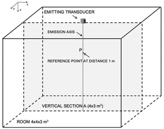
Figure 1.
Simulation setup: the vertical section of the typical 4 × 4 × 3 m3 room along which the ranging calculations using cross-correlation are computed. The SNR is considered at point P, namely at distance of 1 m from the emitter surface center and on its emission axis. Note that the simulation is carried out in a free space scenario with performances evaluated on the plane section A of 4 × 3 m2.
More in detail, the transducer is a circular and planar piston with a diameter of 8.5 mm. This diameter was shown to be able to cover the entire volume of the room using a 30–50 kHz linear chirp signal [18]. For all the simulations that follow, the transducer is divided into small square elements with sides measuring 0.125 mm by 0.125 mm. The chosen element size in this work is a good compromise between the accuracy of the solution and the computational resources involved in the simulations (see Figure 2).
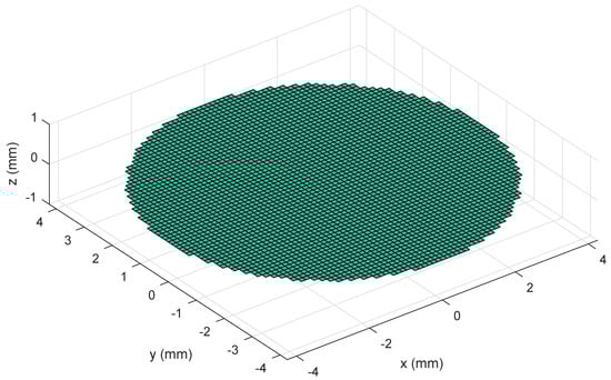
Figure 2.
Emitting transducer: circular and planar piston transducer with a diameter of 8.5 mm divided into 0.125 × 0.125 mm2 square mathematical elements.
A linear chirp with a bandwidth of 30–50 kHz and a duration of 5.12 ms was used as the emitted signal [11,25].
One of the major issues of any ultrasonic ranging system is the environmental noise in the signal band employed.
The approach here proposed allows us to include in the simulation any kind of noise, even the actual disturbance present in the environment for which the system is being designed. On the other hand, when there are no further specific indications, white noise is mostly used for the study of systems in many fields, as it uniformly covers the entire useful band of the system under examination. The use of white noise here is therefore entirely indicative and simply an example.
Uniform white noise was added to the received signal and the reference SNR was calculated at a distance of 1 m from the transducer on its emission axis (see point P in Figure 1). The simulations were carried out in a free space scenario with performances evaluated on the plane section A of 4 × 3 m2, sampling the signal at a frequency fS = 1 MHz.
For an efficient use of the computational resources, the acoustic field was calculated on a regular grid of points in the space for the time strictly necessary, i.e., for the duration of the time window compatible with the complete reception of the employed signal [24], here 15.62 ms, including the chirp duration and the traveling time to the furthest corner of section A in Figure 1.
In a first step, for each considered point in space, the numerical simulation computed the acoustic pressure over the time generated by the complete excitation signal. Subsequently, an ideal receiver, which linearly transduced the pressure signal into an electrical signal, was assumed. This signal was then cross-correlated with the emitted signal at each point and the related ranges were calculated.
The simulations were repeated for different SNR levels and the range errors were computed for increasing noise levels.
3. Numerical Results
In Figure 3, it is possible to see the range estimation error along the section A shown in Figure 1 for decreasing SNR levels from 30 dB down to −20 dB.
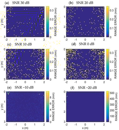
Figure 3.
Numerical results at different SNR levels using a linear chirp 30–50 kHz. A linearized air absorption around 40 kHz has been assumed. Spatial error distribution along the section A of Figure 1: (a) SNR = 30 dB, (b) SNR = 20 dB, (c) SNR = 10 dB, (d) SNR = 0 dB, (e) SNR = −10 dB, (f) SNR = −20 dB. Note the color bar error different ranges. For decreasing SNR from 30 dB down to 0 dB, the error is equal or less than 0.343 mm that is the spatial quantum. For lower SNR error rapidly increases up to more than 500 mm.
The range R is estimated using the usual technique based on finding the position of the cross-correlation peak (τMAX) [17,28]. The adopted technique, in favorable conditions, produces a good estimation of the TOA and, from this, the estimated range R, i.e.,
where τMAX is the lag of the maximum peak of the cross-correlation between the received signal and its copy stored at the receiver (proportional to TOA), TOE is the time of emission of the ultrasonic signal, and Rcal is a calibration constant including all the fixed delays of the system.
In particular, Rcal is range-independent and, together with the TOE, it is assumed to be known through some calibration operations. Finally, cair (m/s) is the speed of sound in the air, which is related to the ambient temperature T (°C) according to:
The ranging error was evaluated on a rectangular grid of points of section A, referring to Figure 1. The grid pitch is 5 cm in the x and z directions. For each point, the lag of the correlation peak (τMAX) and, from these, the distance estimations from the emitter through (1) were obtained. Finally, the ranging errors were computed by subtracting the ground-truth values at each point of the simulation grid from the values just obtained. A typical source of errors in calculating the range is given by the discretization of the τMAX value, with an uncertainty of ±TS/2 according to the time sampling of the system.
In Figure 4a, the overall ranging error at any grid point from Figure 3 is displayed as a cumulative distribution function (CDF) or cumulative error distribution, which is the percentage of readings with error less than the value of a given abscissa. Figure 4b shows a zoomed portion of the CDF in the range 0-5 mm in order to see the behavior details of the ranging mechanism for SNR levels from 30 dB down to −20 dB.
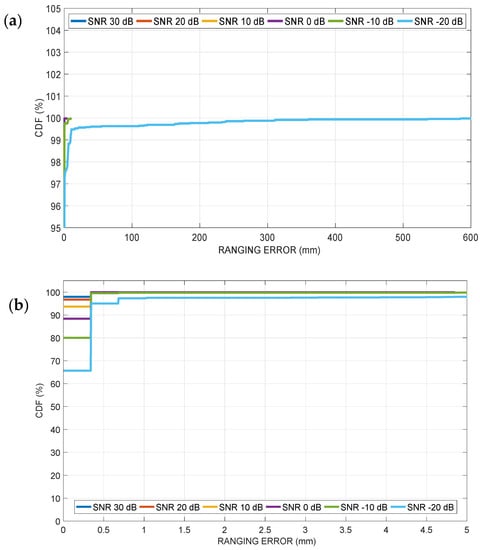
Figure 4.
Numerical results at different SNR levels using a linear chirp 30–50 kHz. A linearized air absorption around 40 kHz has been assumed: (a) cumulative distribution function (percent of readings with error less than the value of a given abscissa) of the ranging error along the vertical section A of Figure 1, for decreasing SNR levels from 30 dB down to −20 dB (y-axis zoomed), (b) x-axis zoomed portion of the cumulative distribution function in the range 0–5 mm.
4. Discussion
Figure 3 and Figure 4 show that the proposed simulative approach allows us to state that the ranging technique based on the cross-correlation achieves a ranging error less than 0.35 mm in every point of the volume in presence of a sufficient SNR level. In detail, in Figure 3a–d, there is a point error pattern, where each point error is limited to one spatial quantum, here equal to TS cair = 0.343 mm for SNR above 0 dB. However, when the SNR drops under 0 dB (Figure 3e,f), the used ranging technique is no longer able to cope with such a high noise level and the error increases up to over 500 mm. In fact, in the presence of high noise levels, the error is mainly due to an incorrect recognition of the peaks, i.e., recognition of a peak as a maximum different from the true one. This error is typically a multiple of the distance between two consecutive peaks in the cross-correlation vector. In the present case, the distance between two consecutive peaks of the cross-correlation is equal to 24 space samples, i.e., about 8.2 mm.
As a significant result, the proposed approach allows us to identify the SNR level that is capable of giving the desired level of ranging error over the entire volume of the room for the transducer and signal shape adopted. Furthermore, the simulation (just an example) shows that it is possible to check whether a particular technique achieves the required performance in the desired space already at the initial design phase.
However, the proposed approach still has significant limitations. In fact, the software tool used for the simulation of acoustic propagation does not consider some effects that are important in the field of indoor ranging. First, the reflection phenomenon is not modeled, and therefore it is not possible at the moment to simulate in a simple way the reflection of the signal, for example, by walls. In other words, phenomena caused by multipath propagation such as self-interference, typical of even a partially reflective environment, are not considered. Secondly, the simulator calculates the propagation as if it occurs in any case in free space and does not consider any obstacles and near-line-of-sight situations. It is therefore not possible to evaluate effectively many situations typical of real applications.
5. Conclusions
In this paper, an acoustic software, originally conceived for in-water simulations of echographic transducers, has been applied to the simulation of the acoustic field in air produced by a circular transducer and to the contextual evaluation of the performance of a ranging technique as a function of the signal-to-noise ratio. The simulations include diffractive and absorption effects in air as a function of the frequency. In particular, the simulations proposed to illustrate the effectiveness of this approach showed that, with a sufficient SNR level, a ranging error of less than 0.343 mm can be obtained in the volume of a typical 4 × 4 × 3 m3 room. This result was obtained using a disc transducer with a diameter of 8.5 mm, a linear chirp signal of 30–50 kHz and a peak detection technique based on cross-correlation. The ranging error is kept within the limit of 0.343 mm when the SNR is greater than 0 dB. For lower SNR levels, the maximum ranging error over the entire volume increases from approximately 0.343 mm to over 500 mm. Some work should be done to make simulation more realistic by including the reflection phenomenon. However, a number of applications and services based on ultrasonic ranging, and therefore on positioning, can already take advantage of the presented approach.
Author Contributions
Conceptualization, R.C.; methodology, R.C.; software, R.C., F.P., M.M., D.I.; investigation, R.C., F.P., M.M., D.I.; resources, R.C.; writing—original draft preparation, R.C., F.P.; writing—review and editing, R.C., F.G.D.C., F.P., M.M., D.I.; visualization, R.C., F.P., M.M.; supervision, R.C., F.P.; project administration, R.C.; funding acquisition, F.G.D.C. All authors have read and agreed to the published version of the manuscript.
Funding
This research received no external funding.
Conflicts of Interest
The authors declare no conflict of interest.
References
- Zafari, F.; Gkelias, A.; Leung, K.K. A survey of indoor localization systems and technologies. IEEE Commun. Surv. Tutor. 2019, 21, 2568–2599. [Google Scholar] [CrossRef]
- Zhang, D.; Xia, F.; Yang, Z.; Yao, L. Localization Technologies for Indoor Human Tracking. In Proceedings of the 5th International Conference on Future Information Technology, Busan, Korea, 21–23 May 2010; pp. 1–6. [Google Scholar]
- Przybyla, R.J.; Tang, H.Y.; Shelton, S.E.; Horsley, D.A.; Boser, B.E. 3D ultrasonic gesture recognition. In Proceedings of the 2014 IEEE International Solid-State Circuits Conference Digest of Technical Papers, San Francisco, CA, USA, 9–13 February 2014; Volume 57, pp. 210–211. [Google Scholar]
- Paredes, A.; Alvarez, F.J.; Aguilera, T.; Villadangos, J.M. 3D indoor positioning of UAVs with spread spectrum ultrasound and time-of-flight cameras. Sensors 2018, 18, 89. [Google Scholar] [CrossRef] [PubMed]
- Fedele, R.; Praticò, F.; Carotenuto, R.; Della Corte, F.G. Instrumented infrastructures for damage detection and management. In Proceedings of the 2017 5th IEEE International Conference on Models and Technologies for Intelligent Transportation Systems (MT-ITSO), Naples, Italy, 26–28 June 2017. [Google Scholar] [CrossRef]
- Merenda, M.; Iero, D.; Carotenuto, R.; Della Corte, F.G. Simple and Low-Cost Photovoltaic Module Emulator. Electronics 2019, 8, 1445. [Google Scholar] [CrossRef]
- Seco, F.; Jimenez, A.R.; Prieto, C.; Roa, J.; Koutsou, K. A survey of mathematical methods for indoor localization. In Proceedings of the 2009 IEEE International Symposium on Intelligent Signal Processing, Budapest, Hungary, 26–28 August 2009. [Google Scholar] [CrossRef]
- Carotenuto, R.; Tripodi, P. Touchless 3D gestural interface using coded ultrasounds. In Proceedings of the 2012 IEEE International Ultrasonics Symposium, Dresden, Germany, 7–10 October 2012; pp. 146–149. [Google Scholar]
- Filonenko, V.; Cullen, C.; Carswell, J. Indoor Positioning for Smartphones Using Asynchronous Ultrasound Trilateration. ISPRS Int. J. Geo Inf. 2013, 2, 598–620. [Google Scholar] [CrossRef]
- Ureña, J.; Hernández, Á.; García, J.J.; Villadangos, J.M. Acoustic Local Positioning with Encoded Emission Beacons. Proc. IEEE 2018, 106, 1042–1062. [Google Scholar] [CrossRef]
- Carotenuto, R.; Merenda, M.; Iero, D.; Della Corte, F.G. An indoor ultrasonic system for autonomous 3D positioning. IEEE Trans. Instrum. Meas. 2019, 68, 2507–2518. [Google Scholar] [CrossRef]
- Sabatini, A.M.; Rocchi, A. Sampled baseband correlators for in-air ultrasonic rangefinders. IEEE Trans. Ind. Electron. 1998, 45, 341–350. [Google Scholar] [CrossRef]
- Aldawi, F.J.; Longstaff, A.P.; Fletcher, S.; Mather, P.; Myers, A. A High Accuracy Ultrasound Distance Measurement System Using Binary Frequency Shift-Keyed Signal and Phase Detection. Available online: http://eprints.hud.ac.uk/id/eprint/3789/ (accessed on 28 April 2020).
- Saad, M.M.; Bleakley, C.J.; Dobson, S. Robust high-accuracy ultrasonic range measurement system. IEEE Trans. Instrum. Meas. 2011, 60, 3334–3341. [Google Scholar] [CrossRef]
- De Marziani, C.; Ureña, J.; Hernández, A.; García, J.J.; Alvarez, F.J.; Jiménez, A.; Pérez, M.C.; Villadangos, J.M.; Aparicio, J.; Alcoleas, R. Simultaneous round-trip time-of-flight measurements with encoded acoustic signals. IEEE Sens. J. 2012, 12, 2931–2940. [Google Scholar] [CrossRef]
- Carotenuto, R. A range estimation system using coded ultrasound. Sens. Actuators A Phys. 2016, 238, 104–111. [Google Scholar] [CrossRef]
- Carotenuto, R.; Merenda, M.; Iero, D.; Della Corte, F.G. Ranging RFID tags with ultrasound. IEEE Sens. J. 2018, 18, 2967–2975. [Google Scholar] [CrossRef]
- Jensen, J.A. Field: A program for simulating ultrasound systems. Med. Biol. Eng. Comp. 1996, 34, 351–352. [Google Scholar]
- Field II Home Page. Available online: https://field-ii.dk/ (accessed on 3 February 2021).
- Carotenuto, R.; Merenda, M.; Iero, D.; Della Corte, F.G. Simulating Signal Aberration and Ranging Error for Ultrasonic Indoor Positioning. Sensors 2020, 20, 3548. [Google Scholar] [CrossRef] [PubMed]
- Tupholme, G.E. Generation of acoustic pulses by baffled plane pistons. Mathematika 1969, 16, 209–224. [Google Scholar] [CrossRef]
- Stepanishen, P.R. The time-dependent force and radiation impedance on a piston in a rigid infinite planar baffle. J. Acoust. Soc. Am. 1971, 49, 841–849. [Google Scholar] [CrossRef]
- Stepanishen, P.R. Transient radiation from pistons in an infinite planar baffle. J. Acoust. Soc. Am. 1971, 49, 1629–1638. [Google Scholar] [CrossRef]
- Jensen, J.A.; Svendsen, N.B. Calculation of pressure fields from arbitrarily shaped, apodized, and excited ultrasound transducers. IEEE Trans. Ultrason. Ferroelectr. Freq. Control 1992, 39, 262–267. [Google Scholar] [CrossRef] [PubMed]
- Carotenuto, R.; Merenda, M.; Iero, D.; Della Corte, F.G. Mobile Synchronization Recovery for Ultrasonic Indoor Positioning. Sensors 2020, 20, 702. [Google Scholar] [CrossRef] [PubMed]
- Bass, H.E.; Sutherland, L.C.; Zuckerwar, A.J.; Blackstocks, D.T.; Hester, D.M. Atmospheric absorption of sound: Further developments. J. Acoust. Soc. Am. 1995, 97, 680–683. [Google Scholar] [CrossRef]
- García, E.; Holm, S.; García, J.J.; Ureña, J. Link Budget for Low Bandwidth and Coded Ultrasonic Indoor Location Systems. In Proceedings of the Indoor Positioning and Indoor Navigation, Guimaraes, Portugal, 21–23 September 2011. [Google Scholar]
- Ens, A.; Reindl, L.M.; Bordoy, J.; Wendeberg, J.; Schindelhauer, C. Unsynchronized ultrasound system for TDOA localization. In Proceedings of the in International Conference on Indoor Positioning and Indoor Navigation (IPIN)), Busan, Korea, 27–30 October 2014; pp. 601–610. [Google Scholar]
Publisher’s Note: MDPI stays neutral with regard to jurisdictional claims in published maps and institutional affiliations. |
© 2021 by the authors. Licensee MDPI, Basel, Switzerland. This article is an open access article distributed under the terms and conditions of the Creative Commons Attribution (CC BY) license (https://creativecommons.org/licenses/by/4.0/).