Article

A Lightweight Dense Connected Approach with Attention on Single Image Super-Resolution

1
College of Information and Electrical Engineering, China Agricultural University, Beijing 100083, China
2
School of Advanced Materials and Nanotechnology, Xidian University, Xian 710061, China
*
Author to whom correspondence should be addressed.
Electronics 2021, 10(11), 1234; https://doi.org/10.3390/electronics10111234
Submission received: 11 April 2021 / Revised: 15 May 2021 / Accepted: 19 May 2021 / Published: 22 May 2021
(This article belongs to the Special Issue Image Fusion and Registration for High-Resolution Image Processing)

Abstract

:
In recent years, neural networks for single image super-resolution (SISR) have applied more profound and deeper network structures to extract extra image details, which brings difficulties in model training. To deal with deep model training problems, researchers utilize dense skip connections to promote the model’s feature representation ability by reusing deep features of different receptive fields. Benefiting from the dense connection block, SRDensenet has achieved excellent performance in SISR. Despite the fact that the dense connected structure can provide rich information, it will also introduce redundant and useless information. To tackle this problem, in this paper, we propose a Lightweight Dense Connected Approach with Attention for Single Image Super-Resolution (LDCASR), which employs the attention mechanism to extract useful information in channel dimension. Particularly, we propose the recursive dense group (RDG), consisting of Dense Attention Blocks (DABs), which can obtain more significant representations by extracting deep features with the aid of both dense connections and the attention module, making our whole network attach importance to learning more advanced feature information. Additionally, we introduce the group convolution in DABs, which can reduce the number of parameters to 0.6 M. Extensive experiments on benchmark datasets demonstrate the superiority of our proposed method over five chosen SISR methods.

1. Introduction

The single image super-resolution (SISR) image processing technique is essential in computer vision and aims to recover a high-resolution image from a single low-resolution (LR) counterpart. It has been used in a large number of computer vision applications, such as medical imaging [1], surveillance imaging [2,3], object recognition [4], remote sensing imaging [5] and image registration and fusion [6,7]. For example, image registration requires high-resolution (HR) images to provide richer details to transform different sets of data into one coordinate system. However, when the upscaling factor increases, the complexity of image registration increases. As a result, it is vital to design an appropriate architecture for the SISR technique.
Traditional SISR methods can be divided into three categories: reconstruction-based methods [8,9], interpolation methods [10,11,12], and learning-based methods [13,14,15,16,17]. Recently, with the rapid development of neural networks, Convolutional Neural Network-based (CNN-based) SR methods have achieved remarkable performances [18,19,20,21,22,23,24]. In 2015, Dong et al. [18] proposed the first Super-Resolution Convolutional Neural Network (SRCNN), introducing a three-layer convolution neural network for single image super-resolution. Afterwards, a Fast Super-Resolution Convolutional Neural Network (FSRCNN) [19] was proposed to accelerate SRCNN, speeding it up by more than 40 times with better restoration quality via a modified network structure and smaller filter sizes. To deal with multi-scale SR problems, Lai et al. proposed a progressive upsampling framework named the Laplacian pyramid SR network (LapSRN) [20], which can progressively generate intermediate SR predictions. Since He et al. [25] presented a Residual Network (ResNet) to show that the network’s depth can be of great significance for various computer vision tasks, some researchers began to increase the network depth to enhance the SR effect. Kim et al. [21] proposed the very deep convolutional network for SR (VDSR). They extended the depth of the network to 20 and achieved higher performance compared with SRCNN and FSRCNN. Soon after, some works [22,23] also successfully demonstrated that deepening CNN networks could further boost SR performance. To alleviate the vanishing-gradient problem brought by the deep network structure, T. Tong et al. [24] proposed a Densely Connected Convolutional Network for SR (SRDensenet) based on dense skip connections, which achieved significant improvement in the image SR task.
SRDensenet has exhibited a good performance at ICCV 2017 due to its contribution to the effective integration of low-frequency and high-frequency features. However, as the network layer deepens, the number of model parameters grows exponentially, dramatically increasing computational complexity. In particular, SRDensenet could waste unnecessary calculations for low-frequency features. The network lacks the ability to identify and learn across feature channels in terms of staking dense blocks, ignoring the inherent feature relationship. Thus, SRDensenet will produce redundant and conflicting information in rich features, which is useless for reconstruction. To resolve the above-discussed issues, in this paper, we propose a lightweight dense connected approach with attention to single image super-resolution tasks, namely, LDCASR, which uses the attention mechanism to learn more effective channel-wise features and the group convolution structure to decrease model parameters. Experiments show that the proposed LDCASR can achieve a better reconstruction performance over the state-of-the-art SISR methods on public SR benchmarks while significantly reducing the model parameters. (About one-ninth of the parameters of SRDensenet.)
In summary, the main contributions of this paper can be summarized as follows.
  • We introduce the attention mechanism to the dense connection structure as well as the reconstruction layer, which helps to suppress the less beneficial information during model training. Extensive experiments verify the effectiveness of this attention-based structure.
  • Our model can extract the important features by using a lightweight approach. By introducing the group convolution, we reduce the number of parameters to 0.6 M, which is around 1/9 of the original SRDensenet.
The remainder of this paper is organized as follows. In Section 2, we introduce the related work of super-resolution tasks and the attention mechanism. In Section 3, we describe the proposed network LDCASR architecture, including the details of its compositions: Recursive Dense Group (RDG), Dense Attention Block (DAB), and Channel Attention Unit (CAU). The experimental results and analysis on the comparison with other methods are provided in Section 4. Finally, we draw our conclusions in Section 5.

2. Related Work

2.1. CNN-Based SISR

Dong et al. unprecedentedly introduced a three-layer CNN framework into the SISR and proposed a super-resolution convolutional neural network (SRCNN) [18], which exhibited a remarkable performance compared to the traditional works [8,9,10,11,12,13,14,15,16,17] and opened the way for neural network-based SR research. After that, plenty of approaches based on convolution neural networks were proposed. A fast super-resolution convolutional neural network (FSRCNN) [19] introduced the deconvolution operation to the CNN model. It not only accelerated the speed but also enhanced the performance of the SRCNN. To further speed up the SR, Shi et al. [26] presented an effective method called efficient subpixel convolutional neural network (ESPCN), which completed the upscaling progress with the aid of subpixel convolution. Lai et al. [20] proposed a progressive upsampling framework called the Laplacian pyramid network (LapSRN) to increase image size gradually. By further deepening the network structure, a very deep super-resolution, VDSR [21], achieved a better result using a deeper network, including almost 20 convolution layers. Afterwards, DRCN [22] and DRRN [23] also realized deep networks by employing recursive learning and sharing parameters. However, with the deepening of the network, the issue of the gradient vanishing appeared. Researchers found the skip connection [25] is a handy way to address the gradient vanishing. Regarding this problem, Ledig et al. [27] proposed residual neural network for SR (SRResNet) with more than 100 layers. They adopted the generator part of the SRGAN as the model structure and employed the residual connections between layers. After that, Lim et al. proposed two even deeper and wider networks: an enhanced deep SR network (EDSR) [28] and a multi-scale deep SR network (MDSR) [28], which both consisted of 1000 convolution layers. These deep SISR networks improve performance by simply stacking the different blocks. However, they ignore the channel-wise feature information. In fact, in addition to the dimension of length and width, the channel is another crucial dimension of an image. Channel attention assigns different weights to each channel to help the network pay attention to important features and suppress unimportant features. With channel attention, the model performance can be improved with a small amount of computation.

2.2. Dense Skip Connections in SISR

To deal with deep model training problems, researchers utilized dense skip connections to promote the model’s feature representation ability by reusing deep features of different receptive fields. The dense skip connections were first proposed in DenseNet [29], which was the subject of best paper in CVPR 2017. Afterward, SRDenseNet [24] exhibited a good performance in SISR by introducing the dense skip connections. Then, many networks employed the dense connected structure in the SR task and exhibited remarkable performances. However, the dense connected structure simultaneously introduces redundant and useless information, which is harmful to the image’s super-resolution. Different from these methods, we combined the dense connected blocks with the attention mechanism to focus on learning important information.

2.3. Attention Mechanism

The attention mechanism was derived from a study of human vision, which was first proposed in the field of visual images. Google Mind team [30] proposed Recurrent Models of Visual Attention in 2014, which used the attention mechanism for image classification on the RNN model. In recent years, attention-based methods have yielded attractive results in various tasks, for instance, image recognition [31] and natural language processing [32]. Researchers found that attention mechanism can not only reduce useless information by discriminating the effective feature information but emphasize the importance in various dimensions. Wang et al. [33] designed a stackable network structure with a trunk-and-mask attention mechanism for image classification tasks. Hu et al. presented a novel block called squeeze and excitation (SE) [34], which employs channel-wise associations using average-pooled features to increase the representational power of a CNN network and ensure accurate image classification. Specifically, the SE block was introduced to deep convolutional neural networks to enhance performance more [35]. Recently, Dai et al. [36] proposed a novel module called second-order channel attention (SOCA) to gain more useful feature expression as well as feature correlation learning. All the methods mentioned above undoubtedly obtained significant results. Inspired by these works, we introduce the attention mechanism to reinforce our network and improve the effect.

3. Our Model

In this section, we first describe the entire architecture of the proposed LDCASR. Then, we introduce the details of different components of the proposed network, including the Recursive Dense Group (RDG) and Dense Attention Block (DAB) with a Channel Attention Unit (CAU).

3.1. Network Architecture

As illustrated in Figure 1, our LDCASR mainly includes three modules: feature extraction module, upscale module, and reconstruction module. We define the original L R input as I L R and the output as I S R .

3.1.1. Feature Extraction Module

The feature extraction module includes a 3 × 3 convolutional layer for shallow feature extraction and several Recursive Dense Groups (RDGs) for deep feature extraction. First, the original low-resolution images were fed into the 3 × 3 convolutional layer straightway to extract the shallow feature. This part aims to transfer the inputs from color space to feature space. The process can be expressed as:
F 0 = H S F ( I L R ) ,
where H S F ( · ) represents the function of the shallow feature extraction process, including only one 3 × 3 convolution layer.
Then, the extracted shallow feature F 0 passed through the stacked Recursive Dense Groups, as well as a 1 × 1 convolution layer to change the number of channels. This process produces the deep image feature, denoted as:
F D F = H D F ( H R D G ( F 0 ) ) ,
where H R D G ( · ) represents the feature extraction operation by RDGs, and H D F ( · ) represents the 1 × 1 convolution operation. Each RDG applies multiple Dense Attention Blocks (DABs) with Channel Attention to suppress redundant information (see Figure 2 and Figure 3), which will be discussed in the following subsection.

3.1.2. Upscale Module

The upscale module was placed after the feature extraction module to upscale the feature maps from small size to the size of ground truth. Instead of merely performing deconvolution or subpixel convolution [26] for upscaling, as in the existing methods, we used channel attention units (shown in Figure 3) and deconvolution operations cross-wise to better capture high-frequency information. Specifically, we used one deconvolution operation in the × 2 experiment, two deconvolution operations in the × 4 experiment, and three in the × 8 experiment.
The low-level feature information includes much original image information, a lot of which will be lost during the process of forward propagation. Thus, it is important to combine the low-level features gained by bicubic-interpolation with the high-level information to obtain the final results. Considering fusing extra original image information, the upscaled features were added to the bicubic-interpolated L R image to acquire the final output of the upscale layer F u p .
The process is expressed as:
F u p = H u p ( F D F ) + B i c u b i c ( I L R ) ,
where the upscale operation is marked as H u p ( · ) .

3.1.3. Reconstruction Module

The final SR image I S R was obtained by the reconstruction module, which contains only one convolution layer of size 3 × 3. This layer aims to recover the images from the feature space to the color space. The reconstruction progress can be expressed as:
I S R = H R ( F u p ) = H L D C A S R ( I L R ) ,
where H R ( · ) denotes the reconstruction layer and H L D C A S R ( · ) denotes the whole process of LDCASR. I S R was optimized by the absolute difference between the I L R and I H R .

3.2. Dense Attention Block (DAB) with Channel Attention Unit (CAU)

As mentioned before, the recursive dense groups (RDGs) are an essential component of our model. Each RDG consists of staked Dense Attention Blocks (DABs) connected by dense connections. It is verified that a large number of dense blocks are beneficial to form a deep CNN in [24]. However, the stacked dense blocks will introduce redundant and conflicting information, causing a longer training time and unsatisfied reconstruction results. Inspired by the methods based on attention, we employed the channel-dimension attention mechanism to learn the high-frequency features and propose the Dense Attention Block (DAB) (see Figure 2), which contains two 3 × 3 convolution operations and a Channel Attention Unit (CAU). As a result, with the aids of DABs, our model is able to focus on acquiring more important and useful information. The progress of DAB can be expressed as:
F n h = f c a t ( f c a u { f c o n v ( f r e l u [ f c o n v ( F n h 1 ) ] ) } , F n h 1 ) ,
where F n h , F n h 1 denote output and input of the h t h DAB in the n t h RDG separately, the operation of convolution, Relu, concatenation and CAU as f c o n v ( · ) , f r e l u ( · ) , f c a t ( · ) , f c a u ( · ) , respectively.
We also denote the input of CAU as F i n and the output as F o u t . The specific formula is as follows:
F i n = f c o n v ( f r e l u [ f c o n v ( F n h 1 ) ] ) ,
F i n = f c a u ( F i n ) = f a v g p o o l ( F i n ) f s i g m o i d ( f c o n v { f r e l u [ f a v g p o o l ( F i n ) ] } ) ,
where f a v g p o o l ( · ) represents the operation of average pooling, f s i g m o i d ( · ) represents the function of sigmoid and ⊗ denotes the element-wise product.

3.3. Group Convolution

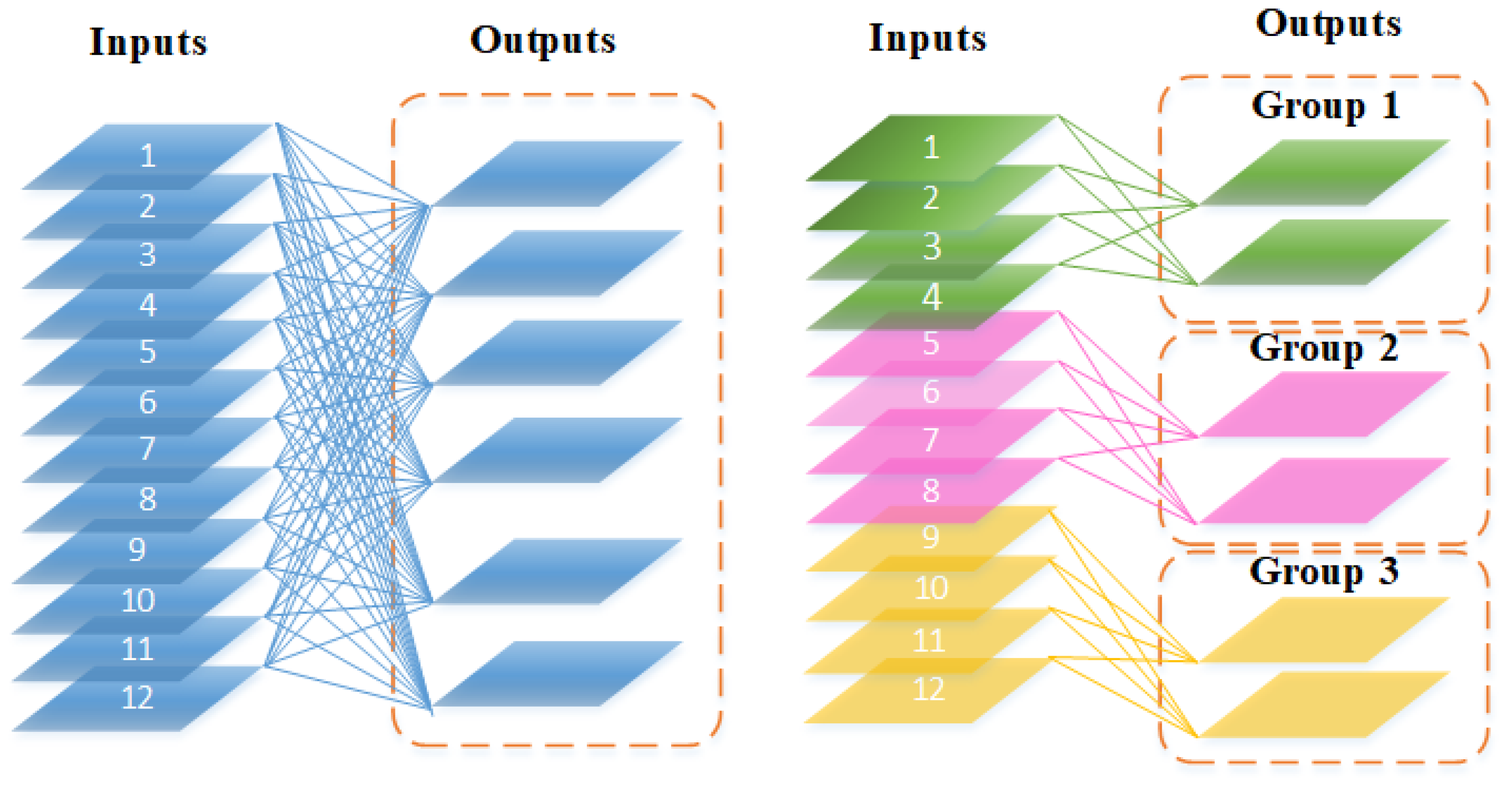
Group convolution first appeared in AlexNet [37] architecture, which is shown in Figure 4. Unlike the standard convolution operation, group convolution can divide all the R channel inputs into G groups, so each group responds to R/G channels. Then, the output is cascaded to the final output of the entire set of convolutional layers. In order to reduce the parameters of the network, we introduced group convolution in each dense attention block (DAB) to achieve a lightweight network.

3.4. Loss Functions

In SISR tasks, loss functions are used to measure reconstruction error and lead the model optimization direction.
In the previous stages, many methods [18,19,20,22,23,25] employ the L2 loss, which is also named the mean square error (MSE) loss. However, researchers found that L2 loss cannot measure the reconstruction quality precisely. Moreover, the result of the reconstruction is not satisfying using L2 loss. Afterwards, more and more researchers tend to use the L1 loss (mean absolute error), which can achieve a better effect of reconstruction. Furthermore, some researchers use the L1 Charbonnier loss function to train the models, which was first proposed in LapSRN. We mark the original high-resolution image as I H R and the loss functions can be expressed as:
L l 1 = ( I S R , I H R ) = 1 h w c n = 1 N I S R I H R ,
L l 2 = ( I S R , I H R ) = 1 h w c n = 1 N ( I S R I H R ) 2 ,
L l 3 = ( I S R , I H R ) = 1 h w c n = 1 N ( I S R I H R ) 2 + ϵ 2 .
where h, w and c represent the height, width and number of channels of the feature maps, respectively. N = h × w × c . ϵ is a constant for numerical stability.
To compare different loss functions, we employed the three loss functions mentioned above to train the LDCASR. The comparison results are displayed in Section 4.

4. Experiments and Analysis

4.1. Training and Testing Datasets

Similar to previous works, our training dataset uses the DIV2K [38]. It consists of 800 training RGB images, 100 validation RGB images, and 100 test images. Following the previous works, we employed 800 training images as our training set, which was then augmented with a 90° rotation and horizontal flip. Furthermore, we used the bicubic kernel function to down-sample the ground truth images to generate LR image counterparts. The training data were generated with Matlab Bicubic Interpolation; training files were created with https://github.com/wxywhu/SRDenseNet-pytorch/tree/master/data, accessed on 11 April 2021.
For testing, we employed four publicly standard benchmark datasets: Set5 [39], Set14 [40], BSD100 [41], and Urban100 [42]. These public datasets provide different kinds of images, which are adequate to validate the models. The test image set was generated with Matlab Bicubic Interpolation; test imageset was created with https://github.com/wxywhu/SRDenseNet-pytorch/tree/master/TestSet, accessed on 11 April 2021.
We followed the previous works by converting the test images from RGB color space to YCbCr color space for evaluation. After that, we employed the peak signal-to-noise ratio (PSNR) and structural similarity (SSIM) to evaluate the performance of our structure only on the Y channel.

4.2. Implement Details

The number of RDB and DAB was set to 8, respectively, identical to the dense blocks and single blocks in SRDensenet. Our model was trained by ADAM optimizer with β 1 = 0.9 , β 2 = 0.999 , the batch size was set to 32, the initial learning rate was 0.0001, and we set the learning rate to the initial LR decayed by momentum every 30 epochs. We conducted our experiment with the scaling factors of × 2 , × 4 , × 8 between the HR and the LR images. We used PyTorch to implement our models with one Titan Xp GPU.

4.3. Different Loss Function Analysis

We show the training results of 60 epochs to compare the training convergence curves of L1 loss, L2 loss, and L1 Charbonnier loss. During the process of gradient descent, the L1 loss was more robust than the L2 loss. Moreover, L1 loss was not easily affected by extreme feature points. This is because the L2 loss function is based on the squared error, which increases twice as much as the L1 loss. As a result, L1 loss is more stable than L2 loss. Additionally, L1 Charbonnier loss adds a variable ϵ 2 compared with L1 loss, making L1 Charbonnier loss more robust than L1 loss. Thus, the learning curve of L1 Charbonnier loss yields the best result. We chose the L1 Charbonnier loss to conduct our following experiments. As shown in Figure 5 and Figure 6, we found that the performance of the training using L1 Charbonnier loss is better than others as its curve is more stable and the average PSNR or SSIM is higher. Therefore, we chose the L1 Charbonnier loss to train our models. The equations of loss functions are shown in Equations (8)–(10).

4.4. SISR Performance Comparison

In this section, we investigate the effectiveness of LDCASR. We compare the average PSNR (dB)/SSIM values with the scale factors × 2 , × 4 , and × 8 on Set5, Set14, BSD100, Urban100.
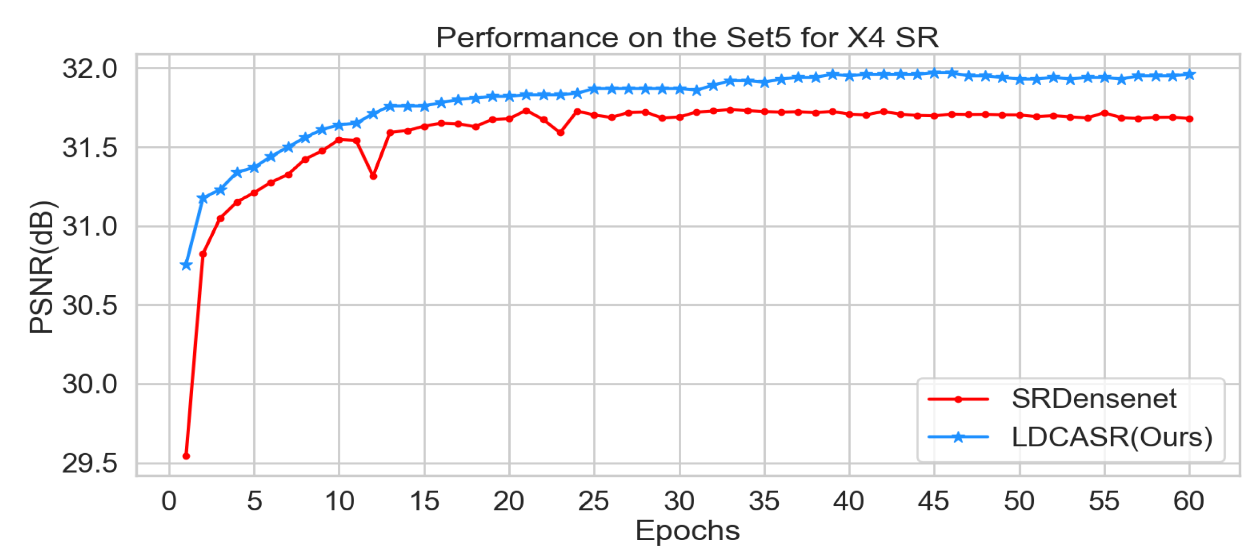
In Table 1, we compare our model with the state-of-the-art methods, including SRCNN, VDSR, LapSRN, and SRDensenet; all the mentioned methods were trained under the same condition. Bold indicates the best performance. As is shown in Table 1, our model achieved was more effective than the other methods under the scale factors of × 2 , × 4 , × 8 on the four benchmark datasets. Obviously, under the × 2 scale factor, the value of PSNR on the Urban100 dataset increased by almost 0.47 compared to SRDensenet. In Table 2, we compare the average computational time of different methods. As can be seen, our LDCASR achieved the second fastest performance for × 2 , × 4 , and × 8 SR experiments, preceded only by SRCNN, which is a simple model with only three convolution layers. Furthermore, we present the performance curve on Set5 for × 4 SR in Figure 7, which intuitively reflects that our model LDCASR is superior to SRDensent. By using the bicubic interpolation, our model exhibited a good performance from the beginning. Subsequently, as the training process continued, the PSNR value of LDCASR stayed at around 32, while the PSNR of SRDensenet stayed at approximately 31.54.
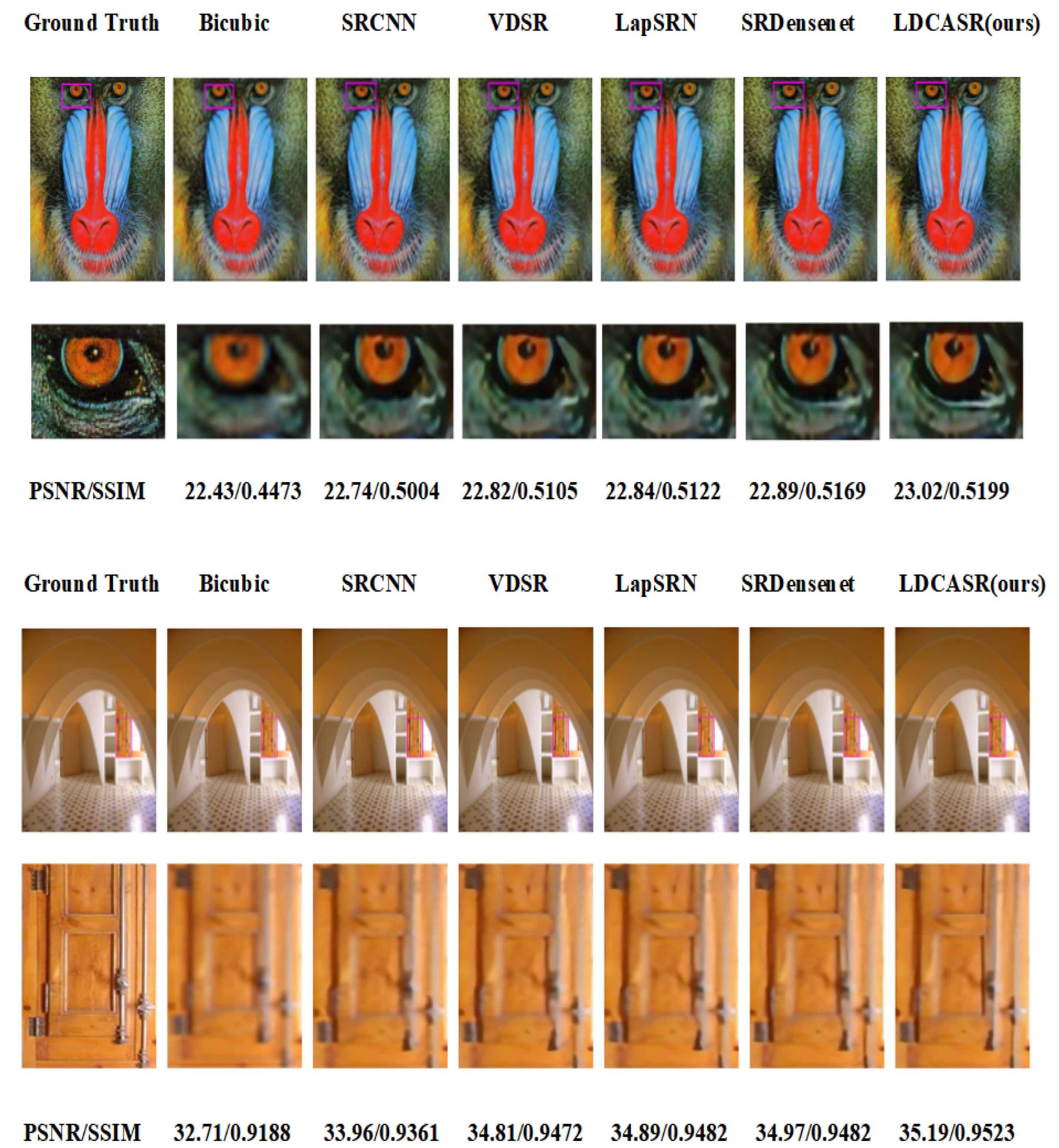
In addition, we provide the comparisons of evaluations in terms of visual quality, which are displayed in Figure 8 and Figure 9.

4.5. Model Size Comparison

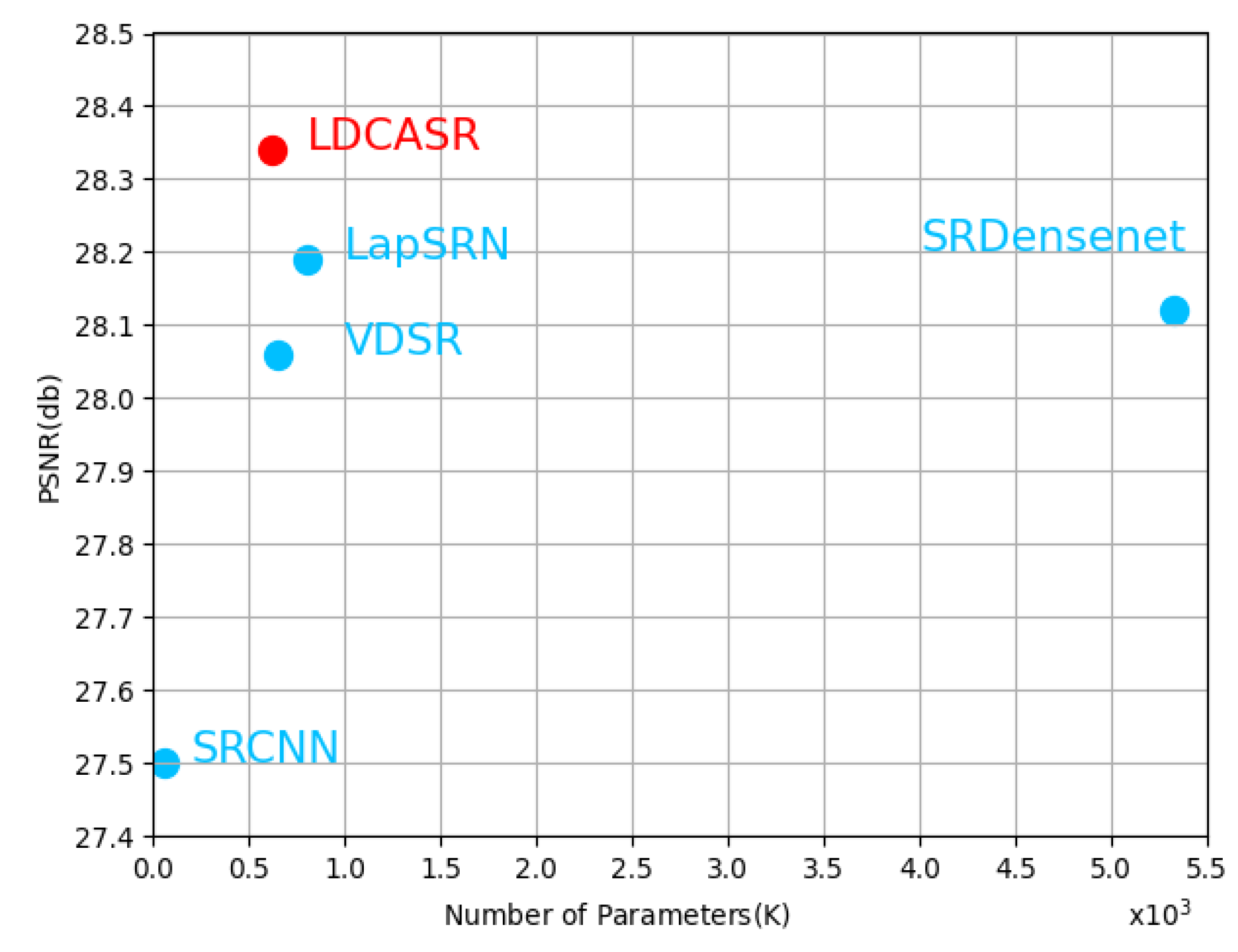
The comparisons of model size and performance are illustrated in Figure 10. It shows the model size and performance of different state-of-the-art methods. The abscissa refers to the model parameter sizes, while the ordinate denotes the image average PSNR obtained by these models, and each point represents a model. The red point represents our proposed network. As can be seen, SRCNN and VDSR exhibited lightweight but slightly lower performances. LapSRN exhibited a better performance than SRDensenet with fewer parameters. Our LDCASR had fewer parameters and exhibited a relatively better performance, which indicates our model achieves a better trade-off between parameter scale and performance.

5. Conclusions

In this paper, in order to solve the deficiency of dense network in the SR task, a lightweight dense connected approach with attention is proposed for SISR, where dense attention blocks (DABs) capture important information in the channel dimension by a channel attention unit (CAU). The design of DABs makes the whole network focus on high-frequency details and successfully suppresses useless information in smooth areas. In addition, our model achieved a lightweight effect with fewer parameters and had a relatively superior performance. The extensive experiments on four benchmark datasets illustrate that our LDCASR achieves better results than other state-of-the-art SR methods in terms of objective evaluation and subjective visual effects. In our future work, we will explore more advanced model structures, such as the model based on improving the spatial attention mechanism or multi-attention mechanism. Moreover, we will study the application of our model in other fields.

Author Contributions

Conceptualization, J.W.; methodology, L.Z. and Z.L.; writing—original draft preparation, L.Z.; writing—review and editing, L.Z. and J.W.; validation, L.Z., Y.Y. and Z.Z.; formal analysis, Y.Y. and Z.Z.; supervision, J.W.; funding acquisition, J.W. All authors have read and agreed to the published version of the manuscript.

Funding

This work was supported by the National Natural Science Foundation of China (No. 61802410).

Conflicts of Interest

The authors declare no conflict of interest.

References

  1. Huang, Y.; Shao, L.; Frangi, A.F. Simultaneous Super-Resolution and Cross-Modality Synthesis of 3D Medical Images Using Weakly-Supervised Joint Convolutional Sparse Coding. In Proceedings of the 2017 IEEE Conference on Computer Vision and Pattern Recognition (CVPR), Honolulu, HI, USA, 21–26 July 2017; pp. 5787–5796. [Google Scholar]
  2. Zhang, L.; Zhang, H.; Shen, H.; Li, P. A super-resolution reconstruction algorithm for surveillance images. Signal Process. 2010. [Google Scholar] [CrossRef]
  3. Rasti, P.; Uiboupin, T.; Escalera, S.; Anbarjafari, G. Convolutional Neural Network Super Resolution for Face Recognition in Surveillance Monitoring. In Proceedings of the International Conference on Articulated Motion and Deformable Objects, Palma de Mallorca, Spain, 12–13 July 2016. [Google Scholar]
  4. Yang, X.; Wu, W.; Liu, K.; Kim, P.W.; Sangaiah, A.K.; Jeon, G. Long-distance object recognition with image super resolution: A comparative study. IEEE Access 2018, 6, 13429–13438. [Google Scholar] [CrossRef]
  5. Mario, H.J.; Ruben, F.B.; Paoletti, M.E.; Javier, P.; Antonio, P.; Filiberto, P. A New Deep Generative Network for Unsupervised Remote Sensing Single-Image Super-Resolution. IEEE Trans. Geosci. Remote Sens. 2018, 56, 6792–6810. [Google Scholar]
  6. Bai, Z.; Li, Y.; Chen, X.; Yi, T.; Wei, W.; Wozniak, M.; Damasevicius, R. Real-Time Video Stitching for Mine Surveillance Using a Hybrid Image Registration Method. Electronics 2020, 9, 1336. [Google Scholar] [CrossRef]
  7. Huang, S.; Yang, Y.; Jin, X.; Zhang, Y.; Jiang, Q.; Yao, S. Multi-Sensor Image Fusion Using Optimized Support Vector Machine and Multiscale Weighted Principal Component Analysis. Electronics 2020, 9, 1531. [Google Scholar] [CrossRef]
  8. Xin, Y.; Yan, Z.; Dake, Z.; Ruigang, Y. An improved iterative back projection algorithm based on ringing artifacts suppression. Neurocomputing 2015, 162, 171–179. [Google Scholar] [CrossRef]
  9. Stark, H.; Oskoui, P. High-resolution image recovery from image-plane arrays, using convex projections. J. Opt. Soc. Am. A 1989, 6, 1715–1726. [Google Scholar] [CrossRef]
  10. Fattal, R. Image upsampling via imposed edge statistics. ACM Trans. Graph. (TOG) 2007, 26, 95. [Google Scholar] [CrossRef]
  11. Keys, R. Cubic convolution interpolation for digital image processing. IEEE Trans. Acoust. Speech Signal Process. 1981, 29, 1153–1160. [Google Scholar] [CrossRef] [Green Version]
  12. Aràndiga, F. A nonlinear algorithm for monotone piecewise bicubic interpolation. Appl. Math. Comput. 2016, 100–113. [Google Scholar] [CrossRef]
  13. Chang, H.; Yeung, D.-Y.; Xiong, Y. Super-resolution through neighbor embedding. Super-resolution Through Neighbor Embedding. In Proceedings of the 2004 IEEE Computer Society Conference on Computer Vision and Pattern Recognition, Washington, DC, USA, 27 June–2 July 2004; Volume 1, p. I-275. [Google Scholar] [CrossRef]
  14. Timofte, R.; De, V.; Gool, L.V. Anchored Neighborhood Regression for Fast Example-Based Super-Resolution. In Proceedings of the IEEE International Conference on Computer Vision, Columbus, OH, USA, 24–27 June 2014. [Google Scholar]
  15. Jiang, J.; Yu, Y.; Wang, Z.; Tang, S.; Hu, R.; Ma, J. Ensemble Super-Resolution With a Reference Dataset. IEEE Trans. Cybern. 2019, 1–15. [Google Scholar] [CrossRef] [Green Version]
  16. Jiang, J.; Xiang, M.; Chen, C.; Tao, L.; Ma, J. Single Image Super-Resolution via Locally Regularized Anchored Neighborhood Regression and Nonlocal Means. IEEE Trans. Multimed. 2017, 19, 15–26. [Google Scholar] [CrossRef]
  17. Yang, J.; Wright, J.; Huang, T.; Ma, Y. Image Super-Resolution Via Sparse Representation. IEEE Trans. Image Process. 2010, 19, 2861–2873. [Google Scholar] [CrossRef] [PubMed]
  18. Dong, C.; Loy, C.C.; He, K.; Tang, X. Image Super-Resolution Using Deep Convolutional Networks. IEEE Trans. Pattern Anal. Mach. Intell. 2016, 38, 295–307. [Google Scholar] [CrossRef] [PubMed] [Green Version]
  19. Dong, C.; Loy, C.C.; Tang, X. Accelerating the Super-Resolution Convolutional Neural Network. In Proceedings of the European Conference on Computer Vision, Amsterdam, The Netherlands, 8–16 October 2016; Volume 9906, pp. 391–407. [Google Scholar] [CrossRef] [Green Version]
  20. Lai, W.-S.; Huang, J.-B.; Ahuja, N.; Yang, M.-H. Deep Laplacian pyramid networks for fast and accurate super-resolution. In Proceedings of the IEEE Conference on Computer Vision and Pattern Recognition, Honolulu, HI, USA, 21–26 July 2017; pp. 624–632. [Google Scholar]
  21. Kim, J.; Lee, J.K.; Lee, K.M. Accurate Image Super-Resolution Using Very Deep Convolutional Networks. In Proceedings of the IEEE Conference on Computer Vision and Pattern Recognition (CVPR), Las Vegas, NV, USA, 27–30 June 2015. [Google Scholar]
  22. Kim, J.; Lee, J.K.; Lee, K.M. Deeply-Recursive Convolutional Network for Image Super-Resolution. In Proceedings of the 2016 IEEE Conference on Computer Vision and Pattern Recognition (CVPR), Las Vegas, NV, USA, 26 June–1 July 2016. [Google Scholar]
  23. Tai, Y.; Yang, J.; Liu, X. Image Super-Resolution via Deep Recursive Residual Network. In Proceedings of the 2017 IEEE Conference on Computer Vision and Pattern Recognition (CVPR), Honolulu, HI, USA, 21–26 July 2017; pp. 2790–2798. [Google Scholar]
  24. Tong, T.; Li, G.; Liu, X.; Gao, Q. Image Super-Resolution Using Dense Skip Connections. In Proceedings of the IEEE International Conference on Computer Vision, Venice, Italy, 22–29 October 2017. [Google Scholar]
  25. He, K.; Zhang, X.; Ren, S.; Sun, J. Deep Residual Learning for Image Recognition. In Proceedings of the 2016 IEEE Conference on Computer Vision and Pattern Recognition (CVPR), Las Vegas, NV, USA, 27–30 June 2016; pp. 770–778. [Google Scholar]
  26. Shi, W.; Caballero, J.; Huszár, F.; Totz, J.; Aitken, A.P.; Bishop, R.; Rueckert, D.; Wang, Z. Real-Time Single Image and Video Super-Resolution Using an Efficient Sub-Pixel Convolutional Neural Network. In Proceedings of the 2016 IEEE Conference on Computer Vision and Pattern Recognition (CVPR), Las Vegas, NV, USA, 27–30 June 2016; pp. 1874–1883. [Google Scholar]
  27. Ledig, C.; Theis, L.; Huszár, F.; Caballero, J.; Cunningham, A.; Acosta, A.; Aitken, A.; Tejani, A.; Totz, J.; Wang, Z.; et al. Photo-Realistic Single Image Super-Resolution Using a Generative Adversarial Network. In Proceedings of the 2017 IEEE Conference on Computer Vision and Pattern Recognition (CVPR), Honolulu, HI, USA, 21–26 July 2017; pp. 105–114. [Google Scholar]
  28. Lim, B.; Son, S.; Kim, H.; Nah, S.; Lee, K.M. Enhanced Deep Residual Networks for Single Image Super-Resolution. In Proceedings of the 2017 IEEE Conference on Computer Vision and Pattern Recognition Workshops (CVPRW), Honolulu, HI, USA, 21–26 July 2017; pp. 1132–1140. [Google Scholar]
  29. Huang, G.; Liu, Z.; van der Maaten, L.; Weinberger, K. Densely Connected Convolutional Networks. In Proceedings of the 2017 IEEE Conference on Computer Vision and Pattern Recognition (CVPR), Honolulu, HI, USA, 21–26 July 2017. [Google Scholar] [CrossRef] [Green Version]
  30. Mnih, V.; Heess, N.; Graves, A.; Kavukcuoglu, K. Recurrent Models of Visual Attention. arXiv 2014, arXiv:1406.6247. [Google Scholar]
  31. Liu, C.; Liang, Y.; Xue, Y.; Qian, X.; Fu, J. Food and Ingredient Joint Learning for Fine-Grained Recognition. IEEE Trans. Circuits Syst. Video Technol. 2020, 1. [Google Scholar] [CrossRef]
  32. Bahdanau, D.; Cho, K.; Bengio, Y. Neural Machine Translation by Jointly Learning to Align and Translate. arXiv 2016, arXiv:1409.0473. [Google Scholar]
  33. Wang, F.; Jiang, M.; Qian, C.; Yang, S.; Li, C.; Zhang, H.; Wang, X.; Tang, X. Residual Attention Network for Image Classification. In Proceedings of the 2017 IEEE Conference on Computer Vision and Pattern Recognition (CVPR), Honolulu, HI, USA, 21–26 July 2017; pp. 6450–6458. [Google Scholar]
  34. Hu, J.; Shen, L.; Sun, G. Squeeze-and-Excitation Networks. In Proceedings of the 2018 IEEE/CVF Conference on Computer Vision and Pattern Recognition, Salt Lake City, UT, USA, 18–23 June 2018; pp. 7132–7141. [Google Scholar]
  35. Zhang, Y.; Li, K.; Li, K.; Wang, L.; Zhong, B.; Fu, Y. Image Super-Resolution Using Very Deep Residual Channel Attention Networks. arXiv 2018, arXiv:1807.02758. [Google Scholar]
  36. Dai, T.; Cai, J.; Zhang, Y.; Xia, S.; Zhang, L. Second-Order Attention Network for Single Image Super-Resolution. In Proceedings of the 2019 IEEE/CVF Conference on Computer Vision and Pattern Recognition (CVPR), Long Beach, CA, USA, 15–20 June 2019; pp. 11057–11066. [Google Scholar]
  37. Krizhevsky, A.; Sutskever, I.; Hinton, G. ImageNet Classification with Deep Convolutional Neural Networks. Adv. Neural Inf. Process. Syst. 2012, 25, 1097–1105. [Google Scholar] [CrossRef]
  38. Timofte, R.; Agustsson, E.; Gool, L.V.; Yang, M.H.; Zhang, L.; Lim, B.; Son, S.; Kim, H.; Nah, S.; Lee, K.M.; et al. NTIRE 2017 Challenge on Single Image Super-Resolution: Methods and Results. In Proceedings of the 2017 IEEE Conference on Computer Vision and Pattern Recognition Workshops (CVPRW), Honolulu, HI, USA, 21–26 July 2017; pp. 1110–1121. [Google Scholar]
  39. Bevilacqua, M.; Roumy, A.; Guillemot, C.; Alberi Morel, M.-L. Low-Complexity Single-Image Super-Resolution based on Nonnegative Neighbor Embedding. In Proceedings of the British Machine Vision Conference (BMVC), Guildford, UK, 3–7 September 2012. [Google Scholar]
  40. Zeyde, R.; Elad, M.; Protter, M. On Single Image Scale-Up Using Sparse-Representations. Lecture Notes Comput. Sci. 2010, 6920, 711–730. [Google Scholar] [CrossRef]
  41. Arbelaez, P.; Maire, M.; Fowlkes, C.; Malik, J. Contour Detection and Hierarchical Image Segmentation. IEEE Trans. Pattern Anal. Mach. Intell. 2011, 33, 898–916. [Google Scholar] [CrossRef] [PubMed] [Green Version]
  42. Huang, J.; Singh, A.; Ahuja, N. Single image super-resolution from transformed self-exemplars. In Proceedings of the 2015 IEEE Conference on Computer Vision and Pattern Recognition (CVPR), Boston, MA, USA, 7–12 June 2015; pp. 5197–5206. [Google Scholar]
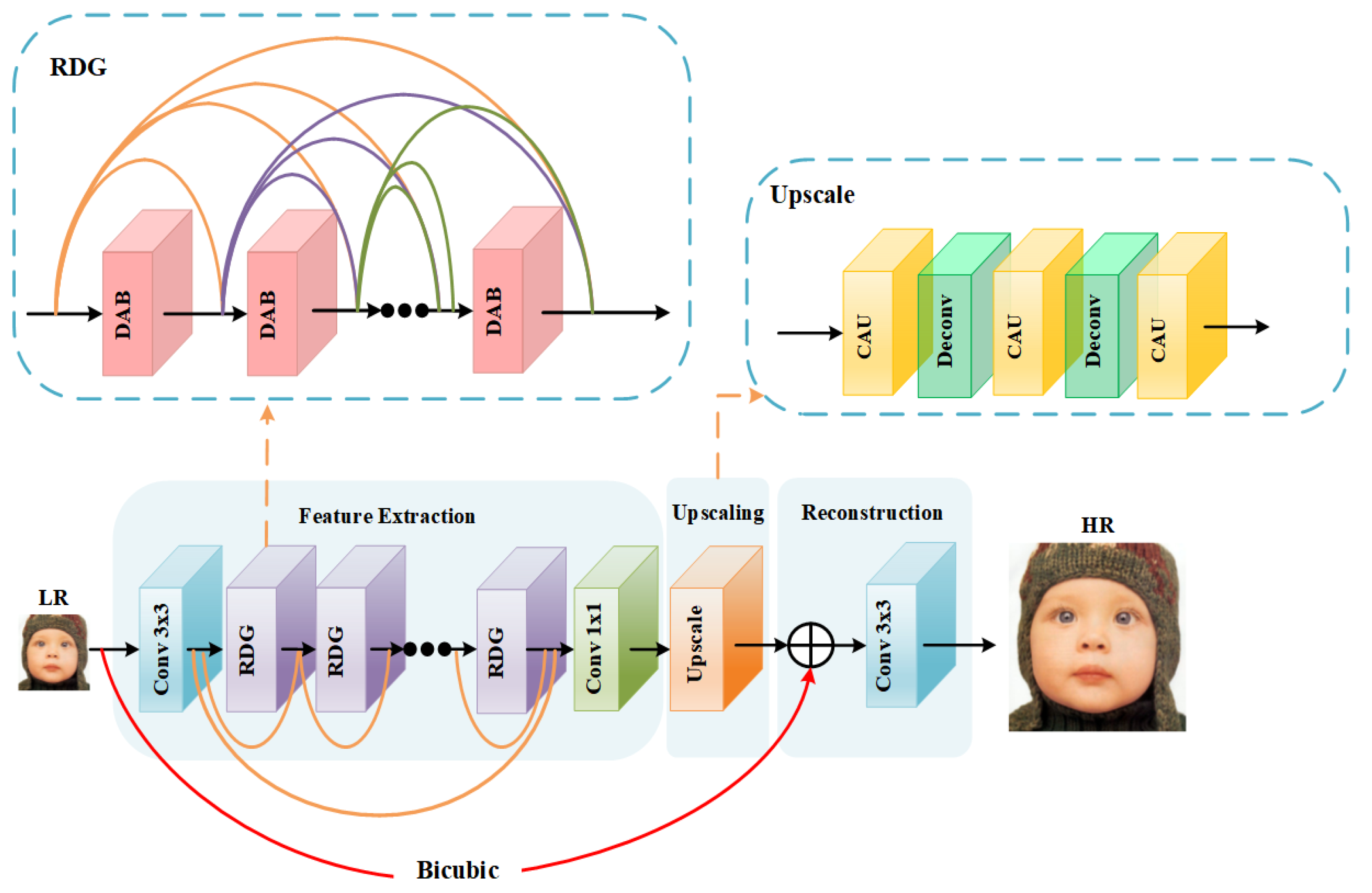
Figure 1. The overall architecture of our model. ⊕ denotes the element-wise product.
Electronics 10 01234 g001
Figure 2. The architecture of the dense attention block (DAB) in RGB. C represents the operation of Channel Concatenate.
Electronics 10 01234 g002
Figure 3. Channe attention unit (CAU). ⊗ denotes the element-wise product.
Electronics 10 01234 g003
Figure 4. Standard convolution (left) and group convolution (right).
Electronics 10 01234 g004
Figure 5. PSNR of networks training with L1, L1 Charbonnier and L2 loss function.
Electronics 10 01234 g005
Figure 6. SSIM of networks training with L1, L1 Charbonnier and L2 loss function.
Electronics 10 01234 g006
Figure 7. Comparison of the performance between SRDensenet and our model.
Electronics 10 01234 g007
Figure 8. Comparison of our models with other works on × 4 SR. The images are from Set14 and Urban100.
Electronics 10 01234 g008
Figure 9. Comparison of our models with other works on × 8 SR. The images are from Set5 and BSD100.
Electronics 10 01234 g009
Figure 10. Performance and number of parameters. Results on Set14 ( × 4 ).
Electronics 10 01234 g010
Table 1. Benchmark results of several state-of-the-art SISR methods.
MethodScaleSet5Set14BSD100Urban100
PSNR/SSIMPSNR/SSIMPSNR/SSIMPSNR/SSIM
Bicubic × 2 33.69/0.930930.33/0.870229.56/0.845126.88/0.8419
SRCNN × 2 36.65/0.954232.45/0.906731.40/0.890229.54/0.8956
VDSR × 2 37.53/0.959033.05/0.913631.95/0.896030.77/0.9140
LapSRN × 2 37.52/0.959133.08/0.913031.08/0.895030.41/0.9103
SRDensenet × 2 37.83/0.960433.26/0.916032.08/0.899431.58/0.9235
LDCASR(Ours) × 2 38.12/0.961833.56/0.918632.21/0.899832.07/0.9288
Bicubic × 4 28.42/0.810426.00/0.702725.96/0.667523.14/0.6603
SRCNN × 4 30.48/0.862827.50/0.751326.90/0.710124.52/0.7221
VDSR × 4 31.42/0.882428.06/0.768927.26/0.726525.21/0.7757
LapSRN × 4 31.54/0.885028.19/0.772027.32/0.727025.21/0.7560
SRDensenet × 4 31.54/0.883428.12/0.771227.32/0.729625.36/0.7640
LDCASR(Ours) × 4 31.94/0.889828.36/0.775827.44/0.732825.77/0.7781
Bicubic × 8 24.39/0.658223.10/0.566023.67/0.548020.75/0.5160
SRCNN × 8 25.34/0.690023.76/0.592624.15/0.566520.73/0.5540
VDSR × 8 25.93/0.724624.26/0.615024.48/0.583621.72/0.5713
LapSRN × 8 26.15/0.738023.38/0.620824.55/0.586521.83/0.5816
SRDensenet × 8 25.92/0.728424.19/0.617824.43/0.585921.73/0.5843
LDCASR(Ours) × 8 26.21/0.738324.43/0.623824.57/0.588621.89/0.5895
Table 2. The average computational time (sec) of different methods on the four benchmark datasets for × 2 , × 4 , × 8 SR. The fastest results are highlighted and our model achieved the second-fastest results.
DatasetScaleSRCNNVDSRLapSRNSRDensenetLDCASR (Ours)
Set5 × 2 0.150360.336250.273461.475260.22986
× 4 0.169080.313960.918621.090840.26533
× 8 0.109120.872210.563850.903530.33260
Set14 × 2 0.234970.654120.476732.758150.43869
× 4 0.254170.626751.039962.168030.46524
× 8 0.214971.757560.543691.139130.48765
BSD100 × 2 0.047760.438240.328611.499760.26857
× 4 0.051590.449110.719451.468240.28653
× 8 0.150371.162500.356620.762870.28375
Urban100 × 2 0.565312.546592.885413.578191.98290
× 4 0.547502.058043.677703.989651.65246
× 8 0.714153.703531.798733.800901.40827
Publisher’s Note: MDPI stays neutral with regard to jurisdictional claims in published maps and institutional affiliations.