Review

AI-Enabled Efficient and Safe Food Supply Chain

1
School of Electrical and Computer Engineering, National Technical University of Athens, 15780 Athens, Greece
2
School of Computer Science, University of Lincoln, Lincoln LN6 7TS, UK
*
Author to whom correspondence should be addressed.
Electronics 2021, 10(11), 1223; https://doi.org/10.3390/electronics10111223
Submission received: 28 April 2021 / Revised: 17 May 2021 / Accepted: 18 May 2021 / Published: 21 May 2021
(This article belongs to the Section Computer Science & Engineering)

Abstract

:
This paper provides a review of an emerging field in the food processing sector, referring to efficient and safe food supply chains, ’from farm to fork’, as enabled by Artificial Intelligence (AI). The field is of great significance from economic, food safety and public health points of views. The paper focuses on effective food production, food maintenance energy management and food retail packaging labeling control, using recent advances in machine learning. Appropriate deep neural architectures are adopted and used for this purpose, including Fully Convolutional Networks, Long Short-Term Memories and Recurrent Neural Networks, Auto-Encoders and Attention mechanisms, Latent Variable extraction and clustering, as well as Domain Adaptation. Three experimental studies are presented, illustrating the ability of these AI methodologies to produce state-of-the-art performance in the whole food supply chain. In particular, these concern: (i) predicting plant growth and tomato yield in greenhouses, thus matching food production to market needs and reducing food waste or food unavailability; (ii) optimizing energy consumption across large networks of food retail refrigeration systems, through optimal selection of systems that can be shut-down and through prediction of the respective food de-freezing times, during peaks of power demand load; (iii) optical recognition and verification of food consumption expiry date in automatic inspection of retail packaged food, thus ensuring safety of food and people’s health.

1. Introduction

Food and drink processing is one of the largest manufacturing sectors worldwide, including all processing steps ‘from farm to fork’ [1]. The economic value of the AI-enabled precision farming market is estimated to grow and reach EUR 11.8 billion by 2025 globally [2]. There are significant challenges within these processing steps, regarding waste reduction, food safety and reduced energy use [3]. Artificial Intelligence (AI) and Machine Learning (ML) technologies offer a transformative solution and recent Deep Learning (DL) approaches have innovated AI-enabled efficient yield and food production, food conservation and supply, reducing food waste and improving food safety.
This paper presents, for the first time, recent progress in the whole pipeline of food production and supply chain. It focuses on three main tasks of the ’from farm to fork’ pipeline: (a) accurate prediction of yield growth and production in greenhouses; (b) optimization of power consumption in food retailing refrigeration systems; (c) quality control in retail food packaging.
At first, accurately predicting yield and food production is of great significance for reducing food waste and achieving smooth supply of food to supermarkets. Crop growers nowadays prefer using greenhouses than field growing. By using greenhouses, growers can extend the growing season and protect crops against changes of weather and temperature. In addition, in greenhouses, environmental parameters, such as temperature, humidity, radiation, carbon dioxide, soil quality and fertilization, can be controlled, providing a safe environment for crop growing [4,5].
Prediction of yield and food production are essential for helping growers control their greenhouse environment and appropriately respond to market supply needs, while reducing operational costs [6,7]. Greenhouse farming operations, yield and production prediction still rely heavily on human expertise. Automated yield and production prediction systems can let growers effectively anticipate weekly fluctuations and avoid problems of both over-demand and over-production arising if the yield cannot be accurately predicted [8,9], constituting an important open research problem [10,11].
According to [12,13] there are two types of approaches, which are based either on the use of existing knowledge, or on extracting correlations directly from data. The former type includes biophysical models for specific species and plants [14,15]. The latter type is based on analysis of large amounts of data aggregated over farms, or greenhouses [16]. In this paper, we focus on recently developed deep learning models, which learn to analyze data, such as humidity, CO2, radiation, outside and inside temperature, together with yield measurements and other plant characteristics, so as to accurately predict the yield, or these characteristics.
In the following phase of the pipeline, food enters the retailing phase, during which it is stored in refrigeration systems of supermarkets. Food refrigeration accounts for a large percentage of electricity demands in developed countries, e.g., it is over 14% of the UK’s electricity demand, and mass refrigeration is responsible for a large percentage of carbon emissions, e.g., around 12% in the UK. When energy consumption exceeds certain limits, this can cause unmanageable spikes in energy usage, with unpredictable problems [17,18]. To reduce load, countries impose response times on large retail energy consumers, requiring them to react urgently, or face high financial penalties. For large companies, with thousands of refrigerators, meeting this requirement relies on staff reactiveness, a highly manualized, resource intensive, non-synchronous procedure.
A procedure to cope with such cases is to turn off some of the refrigerators in such cases for some period of time [19,20]. Using AI and machine learning, it is possible to predict which refrigerators to select and for how long to turn them off, whilst maintaining food quality and safety. In this paper we focus on a deep learning approach that has been recently developed for coping with such situations.
In the third phase of the pipeline, after assuring a safe and efficient storage of food in retailing refrigeration systems, the food is packaged and delivered to the shelves of supermarkets, so that customers can buy and consume it. Serious problems are also met in this phase as well, due to large amounts of food that remain unsold beyond their expiration date. Up to 30% of food is wasted each year, and food poisoning (including over 64,000 annual incidents in the UK from Campylobacter alone) is costly for national healthcare systems and affected individuals [21].
Food manufacturing faces the risk of product recalls and emergency product withdrawals caused by human error on packaging lines; if the expiry date is incorrectly listed as too early, consumers may believe that the product has reached the end of its shelf life and not consume, i.e., waste it. Conversely, if the expiry date exceeds the actual date, consumers may use the product beyond its safe timeframe, risking illness or potential fatality.
Due to prevalence of inkjet printers in food industry, characterized by high degree of quality variability, traditional Optical-Character-Recognition-based vision systems have not been widely implemented, as they struggle with varied or distorted text. In this paper we focus on state-of-the-art deep learning systems that can perform expiry date verification and recognition on photos captured while packaged food passes along production lines [22,23].
The current study is the first to focus on significant problems met within the whole pipeline of food production and supply chain. It presents the use of state-of-the-art machine and deep learning methods for producing an efficient and safe pipeline implementation. It focuses on prediction and recognition tasks of great significance, illustrating the benefits achieved through the use of the machine and deep learning methods. It paves the way for large adoption of AI technologies by growers, retailing organizations and policy makers.
Section 2 presents the methods developed and used to implement the above described frameworks. Section 3 describes the application of the developed deep learning methodologies to real life environments and the achieved performance in all three phases of the pipeline. Discussion of the results that were obtained and description of the future directions are provided in Section 4.

2. Materials and Methods

2.1. Fully Convolutional Networks

Fully Convolutional Networks (FCN) [24] do not contain dense layers, like typical Convolutional Neural Networks (CNN), but contain 1 × 1 convolutions that perform the task of fully connected layers. They are used in the experimental Section for text detection in images. Their architecture includes three parts: a feature extractor stem part, a feature merging branch part and the output part.
The feature extractor stem part is a PVANet [25], including convolutional and pooling layers. In our implementation, four feature maps are extracted from an input image through the convolutional layers, enabling multi-scale detection of text regions of different sizes. Moreover, each pooling layer down-samples a corresponding feature map by a factor of 2.
The extracted four feature maps, f i , i = 1 , , 4 , are then fed in the feature-merging branch part. In the i-th merging stage, the feature map f i 1 obtained in the former stage is fed to an unpooling layer for size doubling and then concatenated with the feature map f i into a new feature map. A convolutional 1 × 1 operator is then applied, followed by a convolutional 3 × 3 operator that produces the merging stage output. Finally, a convolutional 3 × 3 layer produces the merging output and feeds it to the output layer. Multiple convolutional 1 × 1 operations are then used to produce the network outputs.

2.2. Long Short-Term Memories

Long Short-Term Memories (LSTM) are a variation of the Recurrent Neural Network (RNN) architecture [26]. Networks composed of LSTM units have been able to solve the gradient vanishing problem met in long-term time series analysis.
To achieve this, the LSTM structure contains three modules: the forget gate, the input gate and the output gate. The forget and input gates control which part of the information should be removed, or reserved to the network; the output gate uses the processed information to generate the provided output. LSTM units also include a Cell State, which allows the information to be saved for a long time.

2.3. Convolutional–Recurrent Neural Networks

Convolutional–Recurrent Neural Networks (CRNN) are lightweight networks, which are used in the experimental section for text recognition. They include three parts, i.e., a feature extraction part, a bidirectional LSTM-RNN part and a transcription layer part.
The feature extraction part consists of a VGG network [27]. An input image is divided into T different image patches; feature vectors x 1 , x 2 , , x T are extracted from the different patches through convolutional and pooling layers. These feature vectors are then fed to a deep bidirectional Recurrent Neural Network (RNN) composed of recurrent layers with LSTM units. The RNN part can capture contextual dependencies between text in consecutive image patches. It is also able to operate on arbitrary lengths of text sequences.
The final layer in the CRNN is used for transcription, converting the text predictions made by the bidirectional LSTM-RNN into a label sequence. This is achieved through maximization of a conditional probability given the bidirectional LSTM-RNN predictions [28].

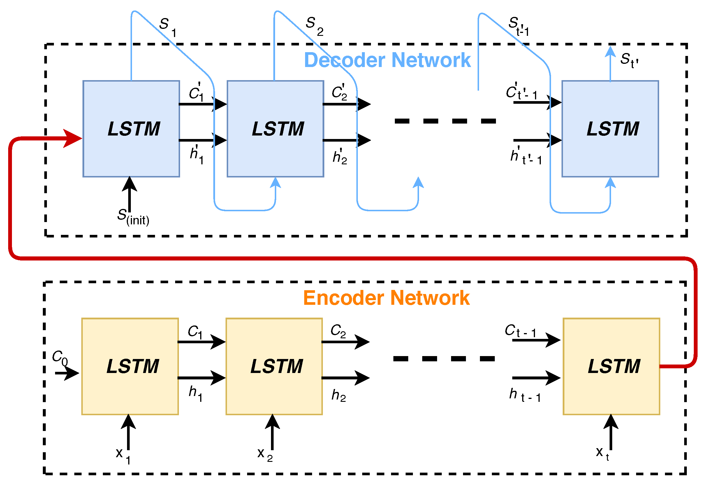
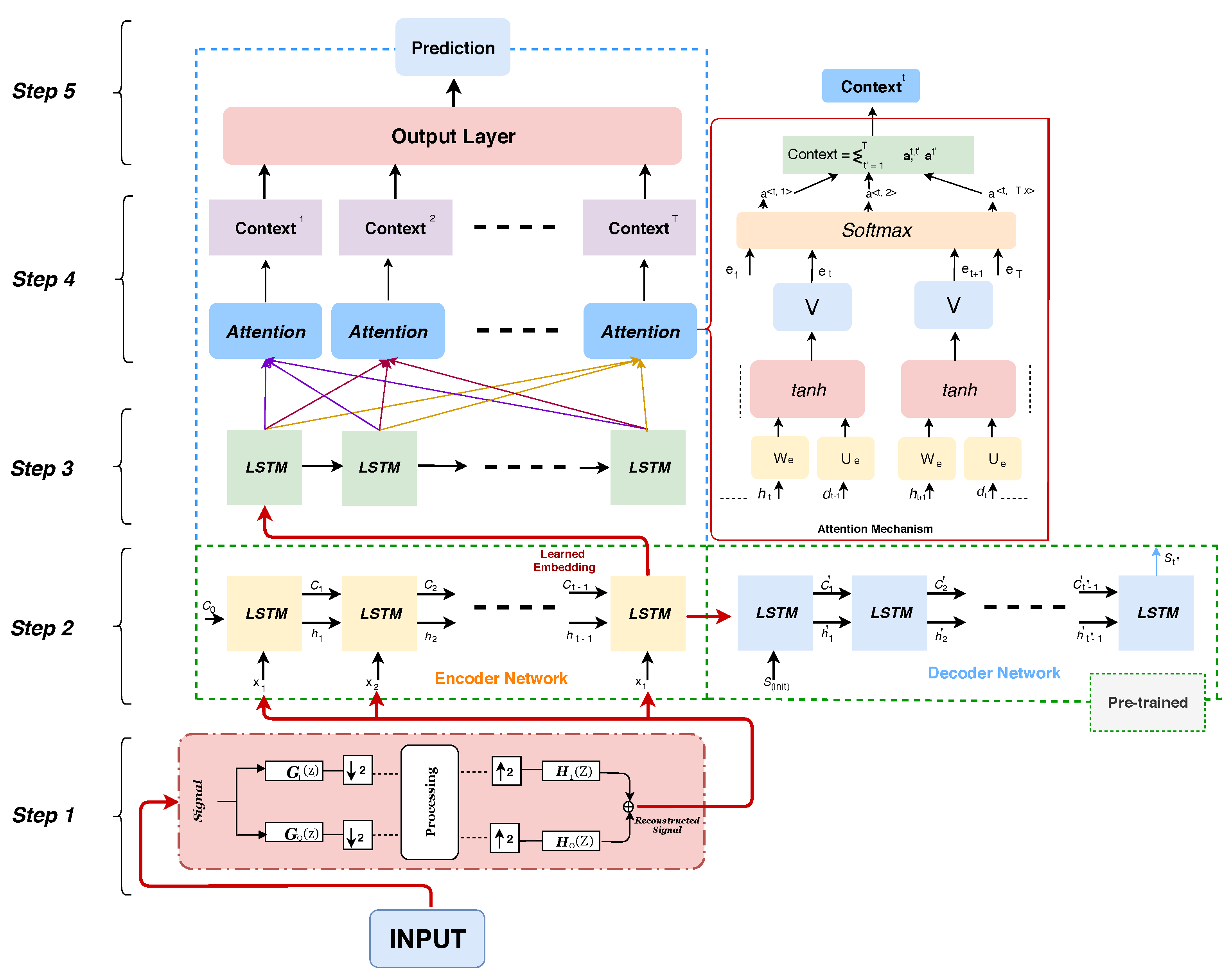
2.4. Encoder–Decoder Model

In LSTM-based encoder–decoder models, the encoder part compresses the information from the entire input sequence into a vector composed of the sequence of the LSTM hidden states. Consequently, the encoder summarizes the whole input sequence ( x 1 , , x t ) into the cell ( C 0 , , C t 1 ) and memory ( h 1 , , h t 1 ) state vectors and passes them to the decoder [29]. The latter uses this representation as initial state to reconstruct the time series ( S t ). The architecture employs two LSTM networks called the encoder and decoder, as shown in Figure 1.

2.5. Attention Mechanisms

Attention mechanisms help to focus on feature segments of high significance [30]. An attention mechanism [31] models long-term dependencies by computing context vectors as weighted sums of all provided information. Such dependencies can be computed across the different internal LSTM layers, as well as over the LSTM output layers.
Output Predictions can be derived using the conditional probability distribution of the input signal and of the previous samples of the output. These are computed in terms of available information (state and input).

2.6. Performance Visualization

Two methodologies are examined in the paper for visualization of the performance of the developed prediction models. These are based on either on class activation maps, or latent variable extraction from trained deep models and adaptive clustering.

2.6.1. Class Activation Mapping

Deep neural networks are usually viewed as black boxes which do not provide means to visualize, or explain, the decision making process. Class activation mapping (CAM) [32] and Gradient-weighted CAM [33] are efficient ways to visualize the significance of various parts of an input image for network training and decision making.
CAM-based methods provide such visualization by generating heat maps for each input image, focusing on the areas that influence the network’s prediction. In practice, they highlight the image pixels which are mainly used for classifying each image to a specific category.

2.6.2. Latent Variable Adaptive Clustering

Extraction of latent variables from trained deep neural networks and generation of concise representations through clustering has been recently used as a means for visualising and explaining the network decision making process [34,35,36].
Let us assume that for each input k, we extract M neuron outputs, as latent variables, from the trained deep neural network, forming a vector v ( k ) . In total, we get:
V = ( v ( k ) , k = 1 , , N
where N is the number of available training data.
We generate a concise representation of the v vectors, that can be used as a backward model, to trace the most representative inputs for the performed prediction. This can be achieved using a clustering algorithm, e.g., k-means, which generates, say, L clusters Q = { q 1 , , q L } by minimizing the following criterion:
Q ^ k - means = arg   min Q i = 1 L v V | | v μ i | | 2
where μ i is the mean of v values included in cluster i.
Then, we compute each cluster center c ( i ) , generating the set C, which constitutes the targeted concise representation:
C = ( c ( i ) , i = 1 , , L
This representation can be used to provide analysis of variability between distributions and adapt information across different food datasets [37].

2.7. Domain Adaptation

Most of the deep learning models are developed through supervised learning over large annotated datasets. However, labeling large datasets constitute a very expensive and time-consuming procedure. Furthermore, in deep learning, it is generally assumed that the training and test statistical characteristics, i.e., distributions, are similar. However, this assumption is not valid in real life environments. This domain shift causes serious problems in the network’s generalisation, requiring model adaptation; this is obtained through Domain Adaptation methods [38].
Many domain adaptation methods have been proposed in the last few years. Three types of approaches, based on Discrepancy, Adversarial and Reconstruction, constitute the means for achieving domain adaptation [38]. The first type aims to align training and test data distributions, minimizing their divergence. This type includes Correlation Alignment (CORAL) [39], Maximum Mean Discrepancy (MMD) [40] and Kullback–Leibler divergence [41] methods. Adversarial methods, based on Generative Adversarial Networks (GANs) [42], aim to achieve the same goal by minimizing domain confusiond [43,44]. The third type of techniques aim to generate shared representations between training and test data, while retaining each domain’s characteristics [45,46].
In the experimental Section we focus on the use of domain adaptation for ensuring safety and waste reduction in the food supply chain. In particular, we target minimization of the discrepancy among features and among class boundaries, as well as minimization of the classification loss, so as to achieve good generalization of the model [22].
The model jointly adapts features combining CORAL and MMD criteria, aligning the underlying distributions. MMD considers the source and target mean embeddings in the Kernel Hilbert Space. The CORAL Loss minimizes the distance between the second order statistics (covariances) of the source and target features.
The total feature discrepancy loss is computed as follows:
L o s s F D = L o s s M M D + L o s s C O R A L
In case we are considering domain adaptation from more than one source domain, the respective models may classify wrongly target data that are close to class boundaries. In such cases, we also minimize the class discrepancy loss among classifiers, L o s s C D [22], making their probabilistic outputs similar. Finally, the classification cross-entropy loss, L o s s C L is additionally minimized during training.
L o s s T O T A L = L o s s F D + L o s s C D + L o s s C L

3. Experimental Study

Figure 2 shows the described AI-enabled Food Supply Chain, including three pillars, which span food production, food storage and maintenance and food distribution and consumption:
-
Food production in greenhouse environments, with a focus on predicting yield and optimizing crop growth and harvesting.
-
Food storage and maintenance in retailing refrigerator systems, with a focus on reducing energy consumption and CO2 production, whilst keeping food safe.
-
Food distribution and consumption with a focus on quality control of retail packaging, through visual inspection of the food expiry date, while aiming to reduce food waste and avoid public health problems.

3.1. Food Production in Greenhouse Environments

3.1.1. Plant Growth Prediction

Machine learning methods are shown to be able to predict growth of Ficus plants using data collected from four cultivation tables in a greenhouse compartment of the Ornamental Plant Research Centre in Destelbergen, Belgium. Greenhouse microclimate was continuously monitored and controlled, through window opening, air heating, assimilation light and CO2 adding. In particular, ficus stem diameter was continuously monitored on three plants and data were collected corresponding to its hourly variation rate, i.e., as the difference between the current stem diameter and the stem diameter recorded one hour earlier. The environmental data were also continuously recorded on an hourly basis.
The prediction problem concerns one-step, two-step and three-step forecasting of the stem diameter [47,48]. In one-step forecasting, stem diameter measurements and environmental data collected, in a time window of the previous 15 h, are used to predict the stem diameter value in the current hour. In two-step-ahead (6 h) forecasting, the above data are used to predict the stem diameter six h ahead. Three-step-ahead (12 h) forecasting makes a stem diameter prediction 12 h ahead.
Figure 3 presents an effective stem diameter prediction method, based on combination of the Encoder–Decoder (ED) model described in Section 2.4, the LSTM model described in Section 2.2 and the attention model (AM) described in Section 2.5 [49].
At first (Step 1), a denoising filter is applied to the input data, composed of the former stem diameter values and the respective environmental parameters. The filter is based on the Wavelet Transform (WT) of the input data, removing the WT high frequency component, and generating a smoothed version of the input data [50]. The ED model is then applied (Step 2). The encoder is pre-trained to extract useful and representative embeddings from the reconstructed time series data. A two-layer LSTM (128 and 32 neurons, respectively) is used in the encoder shown in Figure 1. The decoder learns to generate the (reconstructed) input signal from the embeddings, thus optimizing this feature extraction procedure. Then, the LSTM network, with 128 neurons (Step 3), with an attention mechanism (Step 4), is trained to model respective long-term dependencies, using the learned embedding as input features. A single layer neural network (Step 5) provides the final one-step, or multi-step ahead prediction provided by this WT-ED-LSTM-AM architecture.
In the accomplished experiments, the first 70% of data samples constituted the training set, the next 10% of data samples were the validation set and the remaining 20% of data samples formed the test set. Min–max normalization was applied to the input data, scaling their values in the range [0, 1].
The experimental results illustrate the very good performance of the described method. Table 1 shows that the method outperforms all standard machine learning techniques, including a Support Vector Regressor (SVR), a Random Forest Regressor (RFR), a two-layer LSTM and a Multilayer Perceptron (MLP) with Stochastic Gradient Descent; a learning rate ls = 0.001 and a batch size of 32 were adopted. All models were trained for 100 epochs, using the same training, as well as validation and test data sets. The Root Mean Squared Error (RMSE) was used as performance evaluation criterion. To illustrate the contribution of the WT and AM steps, Table 1 also illustrates that the achieved performance becomes worse, if either of these two steps is not included in the prediction approach.
Figure 4 shows the accuracy of Ficus growth one-step prediction by all methods for about 600 data samples. It can be seen that the described model successfully performs one-step ahead prediction, outperforming the other methods and providing accurate estimates of almost all peak values in the original data.

3.1.2. Yield Prediction

Modeling the growth of tomato crops in greenhouse environments has been the topic of some related research [51,52]. These models are physics-dependent and are based on large numbers of related parameters. They are rather complex, with difficulty in estimating initial parameter values and need calibration in every environment.
The Tompousse model [14] was developed taking into account the fruit weight and linearly relating it flowering rate. Another tomato yield model [15] represented weekly yield fluctuations in terms of fruit size and harvest rate [53].
Machine learning models have been recently developed for tomato yield prediction [54]. Their training was conducted with data aggregated from Greenhouses in United Kingdom, over a period of two years. The data contained environmental parameters and actual yield values.
Environmental data were collected every hour, while yield values were collected once per week. To make the data consistent in terms of time of occurrence, data augmentation was accomplished, using interpolation, on the yield measurements. This resulted in yield values on a daily basis. Moreover, by averaging the environmental data, we generated environemntal data on a daily basis as well.
The experimental study on these data illustrated the ability of the above-described ED-LSTM-AM model (WT did not provide any significant improvement in this case) to provide accurate prediction of tomato yield. Figure 5 shows that this model outperforms standard ML methods, including SVR and RFR, in tomato yield prediction. The MSE in actual yield prediction was 0.015 for SVR, 0.040 for RFR and only 0.002 for ED-LSTM-AM.

3.2. Food Retailing Refrigeration Systems

Applying deep learning methods in distributed environments is still an open research and development problem. Examples of current distributed frameworks include TensorFlow-distribute, or IBM distributed DL. Sharing data in distributed environments, while implementing, for example, the LSTM networks described in Section 2.2, is a critical bottleneck, despite the prevalence of databases providing very mature and advanced functionalities, such as MongoDB’s aggregate pipeline. There are different types of parallelism in deep learning implementations [55], as listed below:
-
Model parallelism (TensorFlow, Microsoft CNTK), where a single deep model is trained using a group of hardware instances and a single data set.
-
Data parallelism, where each hardware instance is trained across different data.
-
Hybrid parallelism, where a group of hardware trains a single model, but multiple groups can be trained simultaneously with independent data sets.
-
Automatic selection, where different parts of the training/test process are tiled, with different forms of parallelism between tiles.
In the food supply chain, machine learning methods can be effectively used in a hybrid parallel framework for controlling massive amounts of food retailing refrigeration systems. This was shown in a recent implementation [56], in which multiple LSTM models were coupled with a MongoDB database [57] and were trained, using 110,000 real-life datasets—from about 1000 refrigerators.
The generated Nemesyst system [58] has been capable of predicting which refrigerators to select and how long to turn them off, whilst maintaining food quality and safety. This was implemented in a Demand Side Response setting that modified power demand load proportionally to available energy, in the National Grid of the United Kingdom [59,60]. The target of the research was to show how to optimise refrigeration systems with machine learning at scale, whilst assuring that food temperature did not exceed certain thresholds.
The Nemesyst system simultaneously wrangles, learns, and infers various models, over different data sets, within a network of refrigerator systems. In such systems the thermal inertia/mass of food acts as a store of cold energy. However, the thermal inertia in a retail refrigeration case changes, if food is actively shopped by consumers and then refilled, if the ambient temperature changes, if networks of stores possess multiple refrigeration systems, or if different types of food need specific control mechanisms [61,62].
Deep learning models, such as LSTMs, can model thousands of assets simultaneously, whilst being retrained to decide which refrigerators to turnoff, within a large network of refrigerator systems. This requires an algorithm that can predict the thermal inertia in individual cases and therefore how long they can be shutdown (typically up to a maximum of up to 30 min), ensuring food safety and contributing to decarbonisation.
As shown in Figure 6, a backend deep learning framework aggregates data from a distributed global database layer and trains with them multiple deep models, such as LSTMs. It then stores the trained models in the database layer. The latter interacts with each local store and its refrigerator systems, which share local database instances and retrieve the best deep network from the global database layer.
In the experimental study the target was to predict the time that each refrigerator’s temperature needed to rise from the turn-off time until reaching a critical, for food safety, temperature. This time was different in different cases, ranging from 8 °C for high temperature refrigerators to −183 °C in low temperature freezers. The threshold for each fridge was not a-priori known. To face this problem, a two-layer LSTM network was trained to predict the defrost time point, since this point was the most appropriate for the task.
A number of 110,000 refrigerators was selected from the whole population and used in the experimental study. Predicting how long the refrigerators could remain off, before reaching this threshold, identified the best candidates so as to reduce the power consumption and minimize the number of affected refrigerators and potentially affected food. The 110,000 defrost examples were split such that 10,000 were used for final testing, 10,000 were selected each time for validation and the rest were used for training the system.
Figure 7 illustrates that an excellent prediction of the defrost time was achieved in four different cases. The time for defrosting before reaching the temperature of 8 °C was computed as the difference between the last “observed” and final “defrost” value. In cases (a) and (b), prediction defined exactly the point of defrost; in cases (c) and (d), prediction took place two minutes before defrost.

3.3. Quality Control in Retail Food Packaging

The requirement for food high quality and safety of food and the public is a very important issue throughout the whole food supply chain [63]. The food product information printed on the food package is very important for food safety. Incorrectly labelled product information on food packages, such as the expiry date, can cause food safety incidents, such as food poisoning. Moreover, such faults will incur high reputational and financial cost to food manufacturers, also causing large product recalls. As a consequence, verification of the correctness of the expiry date printed on food packages is of great significance.
In the following, it is shown that, instead of relying on operators to check the date code, an automated solution, taking photos of each date code, can verify the programmed date code for that product run, allowing food processing businesses to introduce unmanned operations and achieve very high inspection with full traceability, without compromising product safety. The production line will stop if the date code is incorrect, ensuring that the respective products are not released into the supply chain, protecting consumers, business margins and their brand, while reducing labour costs and food waste.
The Food Packaging Image dataset used next consists of more than 30,000 images classified in two categories (existing valid date and non-existing or non-valid date) from six different locations in the Midlands in the United Kingdom. A total of 70% of the data were used for training the model; 10% were used for validation and 20% formed the test set. Representative images are shown in Figure 8, showing a complete date (a), partial dates (b,c), an unreadable date (d) and no existing date (e).

3.3.1. The FCN-CRNN Approach for Expiry Date Recognition

Optical character recognition (OCR) systems [64,65] can be applied to automatically recognize expiry date characters based on food package images captured by RGB cameras. However, existing OCR systems can not achieve high performance in real-world expiry date recognition scenarios, which include high variability, different fonts/angles, complicated designs with rich colours/textures, blurred characters poor lighting conditions in food manufacturing/retailer sites. Deep neural networks have been recently used as a means to tackle such problems [66,67].
In the following we present an approach composed of the FCN network described in Section 2.1 and the CRNN network described in Section 2.3. Both networks are lightweight and have achieved good performance in text detection and recognition `in-the-wild’. Thus, they were fine-tuned and combined together to detect and recognize the expiry date. Fine-tuning is performed through transfer learning [68], by adapting the model, pre-trained for recognition of text, to recognition of the expiry date.
The FCN-RCNN architecture is shown in Figure 9. It includes the FCN part, which is responsible for the detection of the Region-Of-Interest (ROI) of the expiry date. This acts as a filter to identify the image patch including the ROI from a whole food package photograph, so that the recognition task is performed on that specific small image patch, instead of the whole image. The second part includes the CRNN network, which performs date character recognition on the image patch obtained from the first network. Multiple levels of features are extracted from equally divided regions in the expiry date ROI, so as to recognize the characters within each region, while contextual relationships between characters in consecutive regions are modelled by the recurrent layers of CRNN.
The accuracy of expiry date detection by the fine-tuned FCN model reaches 98.2%. It is higher than the accuracy obtained with two other similarly fine-tuned popular deep neural networks, i.e., CTPN [69] and Seglink [70], while providing much fewer false alarms and missed detections, as shown in Table 2.
Then the CRNN part of the method was fine-tuned using annotated (rectangular) image patches extracted by the FCN part. As shown in Table 3, the achieved recognition accuracy was 95.44%, much higher than that provided by the Tesseract OCR tool [71] and higher than the performance of the TPS-ResNet-BiLSTM-Att network [72], which is much more complex (containing six times more parameters than the CRNN model).

3.3.2. Latent Variable Based Expiry Date Verification

A high variability exists in the image characteristics captured in different environments. As a consequence, an FCN model trained with images from a dataset collected in one location did not perform well when applied to images collected in another location. A method to cope with this problem is by extracting latent variables from each trained FCN, clustering them as described in Section 2.6.2 to produce respective cluster centroids and using these centroids as an equivalent model for evaluating images from other locations through nearest neighbour classification [37].
It has been shown that best results were achieved in this way, if latent variables were extracted by the dense layer preceding the output network layer [35,36,73]. For this reason, some dense layers were included on top of the FCN network, as shown in Figure 10. In particular, an averaging pooling and two dense layers, each containing 2048 ReLU units were added and the 2048 neuron outputs of the last dense layer were clustered using the k-means algorithm.
Let us consider the case of two datasets obtained from different locations. Seven clusters were generated per dataset [37], after applying the above procedure to each dataset. The respective 14 centroids were then merged, following an algorithm based on [35,74], which iteratively removed the lowest performing cluster, resulting in adaptation of some of the remaining centroids, until the expiry date verification stopped improving.
Figure 11 shows the effect of the algorithm on the 14 original cluster centoids. Two of them (black stars) were excluded; four centroids (red squares) in class 1 and two (green circles) in class 2 were adapted and the rest of the CNN centroids remained unaffected. It should be mentioned that this produced an improvement in the verification accuracy of 13.8% in total accuracy over the datasets of the two locations.

3.3.3. Domain Adaptation for Multi-Source Expiry Date Recognition

The problem of high variability across datasets collected in different environments, which was tackled in the former subsection, as well as the general lack of labeled data for the whole food supply chain, was further examined next, using the domain adaptation approach described in Section 2.7.
Figure 12 shows the developed domain adaptation procedure. It included a feature extraction and a classification part. The feature extraction part and its sub-networks were trained to learn features that represented every source–target relation. The classification part was trained to learn domain-specific attributes for every image in the target set. A Class Activation Map was included, as described in Section 2.6.1, to provide visualization of which parts of the input images most affected the provided predictions.
Experiments were conducted using a labeled single source dataset and an unlabeled single target dataset for all six locations. The goal of this experiment was to establish a baseline for images that would be classified as readable and acceptable according to human standards. Further experiments were conducted using the multi-source domain adaptation approach, in two settings, i.e., of two source and one target, or three source and one target datasets.
For comparison purposes, more experiments were implemented, in which the two, or three source datasets were combined in a single source dataset; this was then used for domain adaptation to the target dataset. In the experiments, either the FCN—or the ResNet-50 [75] pretrained on ImageNet [76]—was the backbone network, by adding a dense layer and fine-tuning all convolutional and pooling layers.
Table 4 presents the average classification accuracy for all examined domain adaptation methods. As shown in the Table, combining two, or three sources provided better results than single source methods. This can be justified by considering this case as data enrichment. Moreover, the multi-source domain adaptation method significantly outperformed both other methods. The improvement of the average classification accuracy was over 6%.

4. Discussion

The presented experimental studies illustrated that the use of AI and ML methodologies can provide the food supply chain with efficiency and safety, reducing food waste and environment pollution; this is the main target of the data platforms required for food systems [77,78]. Most of the presented work has taken advantage of the recent progress in deep learning and deep neural networks.

4.1. Food Production in Greenhouses

In the first case study, DL systems were trained to predict growth and yield in time series data collected in greenhouses, taking into account environmental data and historical growth, or yield data. It has been shown that RNN/LSTM models combined with autoencoding, or attention mechanisms, were able to provide state-of-the-art performance compared with existing methods for multi-step prediction of stem diameter-based growth of plants, as well as of tomato yield weekly prediction. Similar approaches can be used for prediction of yield of other categories, for example fruits, and in particular strawberry yield and their harvesting using robots [79,80]. In addition, simultaneous maximization of yield and minimization of the consumed energy in greenhouses can be tackled through dynamic multi-objective optimization [81,82].
Based on the presented analysis, we can foresee the following future developments, relating market dynamics with food supply–demand balance.
It is crucial for greenhouse farmers to harvest their produce in perfect condition at the right time and make them onto the food market to maximise profit while helping stabilise the supply chain. Normally, farmers pick their produce while they are still green and induce the ripening process afterwards by spraying the fruits or vegetables with ethylene gas when they reach their destination. These post-harvest practices have drawbacks; fruits harvested prematurely may result in poor taste and quality despite appearing as fully ripened ones, particularly for ethylene-sensitive vegetables including broccoli, cabbage, and lettuce. This is further compounded by high aesthetic standards in today’s market—only the best-looking produce makes it on to supermarket shelves. Fruit and vegetables of low quality cannot be sold, which creates waste and unnecessary expense for farmers. On the other hand, natural ripening processes in greenhouses are costly, due to extra heating and lighting at the end of the season.
Improvement of natural ripening processes can be achieved by optimising climate parameters in greenhouses, so that crops are harvested at the best time to meet market demand and maximise profit. To reach this aim, we will need to perform more research on: modelling correlation of natural crop ripening with greenhouse climate parameters, such as temperature, humidity, CO2 and soil environment parameters; using market dynamics to inform ripening control; optimising climate control in ripening processes to maximise profit and minimise carbon footprint simultaneously.
This research will include: using the deep learning models presented in the paper to elucidate the relationship between crop ripening and greenhouse climate and soil environment parameters; integrating market demand forecast into greenhouse climate control during crop ripening process; using machine learning for dynamic multi-objective optimization of greenhouse climate control during crop ripening processes to maximally increase profit and lower CO2 emission.
Other multi-objective optimization models can be related to these developments. Such a model is the linear programming model developed in [83] for designing a citrus three-echelon supply chain network. This model minimizes waste, transportation and inventory holding costs, while maximizing profit. Another model [84] considers a four-echelon citrus supply chain, including gardeners, distribution centers, citrus storage and fruit market. This is a mixed integer non-linear programming model, which minimizes total cost and maximizes profit.

4.2. Food Storage and Maintenance in Refrigeration Systems

In the second case study, it has been shown that control of the energy consumed by big food suppliers, e.g., large supermarket companies, is feasible, using deep learning based prediction. A large scale study, for automatic control, i.e., temporary shutdown of retailing refrigerator systems in peak energy demand hours, has been implemented, based on prediction of the specific refrigerator defrost period in each considered location. RNN/LSTM models were mainly used to perform the prediction task; GAN models were also successfully used to perform data augmentation and prediction. Similar methods have been used to predict anomalies, i.e., instances when the power demand load becomes higher than the available power in a country [85].
Current targets related to food supply chain, worldwide, include [3]: cutting of greenhouse gas emissions by at least 55% by 2030; development and use of energy-efficient approaches; optimization of connectivity to energy; analysis of production data; efficient management of resources, such as energy, water, soil, biodiversity. The presented approaches illustrate how AI and DL can be used to contribute towards these goals.
Achieving this goal requires setting up of a respective policy, which can be achieved through a combined top-down and bottom-up procedure. On the one hand, states should encourage the use of AI-enabled energy control approaches by big players in the food supply food market. On the other hand, smaller and larger food market players should adopt such solutions, so as to maximize efficiency and safety of the food production and supply chain. The outcome of this dual adoption of AI-enabled procedures will be creation of a complete food production and supply pipeline that takes into account health and environmental constraints, as well as the information and economic needs of all involved stakeholders, including farmers, retailers and customers. In this framework, design of a complete interactive interface system that can integrate all these needs, while creating a good user experience, is of major importance.
The presented model can be combined with other types of models, such as the hub location-vehicle scheduling model [86], which considers perishability of products for distribution in a food supply chain and total CO2 emission of the hub, simultaneously. The underlying multi-objective optimization takes into account total transportation costs, freshness and quality of foods at the time of delivery and total carbon emissions of vehicles. Another model that can be taken into account [87] refers to environmental sustainable issues connected with agro-food supply chain from farmer to final distribution centers. This model minimizes the total transportation cost and carbon emission tax in gathering food grains from farmers to the hubs and later to the selected demand points (warehouses).

4.3. Food Distribution and Consumption

The third case study illustrated that automatic recognition of expiry date in retail food packaging can also be successfully implemented through deep learning methodologies. It was shown that FCN and CRNN models can be used to effectively recognize the expiry date on real life food packaging. Verification of the expiry date, with visualization of the decision making procedure can be achieved through latent variable extraction of the trained deep neural architectures and a related clustering procedure. Moreover, domain adaptation of the deep neural architectures can be performed so as to achieve expiry date verification and recognition across different retail environments.
The impact of this task is also crucial for ensuring food safety and consumers’ health, whilst reducing food waste and related financial loss. Supermarkets can be automatically informed and perform respective early warning pushes, or notifications before the expiration dates, combined with retail sales and other activities to reduce food waste.
The presented deep learning approaches may be applied to other significant tasks in monitoring retail food packaging. In particular, they can provide verification and recognition of the allergen labeling barcode, or other nutritional information. These can create a further impact towards people’s safety, by automatically informing customers which allergens are included in the food products they are thinking of buying in retail supermarkets.
All the above experiments used the state-of-the-art in deep learning methodologies. In future research, the developments will focus on extending the described frameworks, with a target to combine deep learning with AI knowledge representation and reasoning, as well as multi-objective optimization technologies [88,89].
In this context, the methodologies that were presented in this paper for achieving an efficient and safe food supply chain will be extended, so as to create trustworthy AI-enabled food chain supply, that offer transparency and explainability to their users, i.e., food producers and farmers, retail supermarket owners, customers and the general public.
In particular, the deep neural architectures, especially the approach deriving the backward model of extracted cluster characteristics, described in Section 3.3.2, can be interweaved with ontological representation [90] of this backward model, so as to provide explainable cues of the decision making procedure by using query answering techniques [91,92].
Justification and explanation of the decision making procedure is of great significance for creating trust of stakeholders in the developed AI-enabled predictions and suggestions. For example, in the case of farmers, if the AI system predictions conflict with their experiences, the system should be able to provide visualization and explanation of the input characteristics on which its prediction was based. Moreover, it should be able to link this justification with former experiences of the specific farmer, or of other farmers in similar contexts, so that the farmer continues to believe and use the system. In this framework, the derived models should be able to adapt and contextualize across different environments; general-purpose methodologies developed for other classification and prediction fields [93,94] can be used to achieve this capability.

Author Contributions

The individual contributions of the authors are as follows: conceptualization, S.K.; methodology, I.K.; software, J.S.; validation, S.K., J.S.; formal analysis, I.K.; writing—original draft preparation, I.K. and J.S.; writing—review and editing, S.K. All authors have read and agreed to the published version of the manuscript.

Funding

This research received no external funding.

Conflicts of Interest

The authors declare no conflict of interest.

References

  1. European Commission Communication. A ‘Farm to Fork’ Strategy for a Fair, h. Environmentally-Friendly Food System (COM (2020) 81 Final). Available online: https://eur-lex.europa.eu/legal-content/EN/TXT/?uri=CELEX:52020DC0381 (accessed on 27 April 2021).
  2. European Commission Sectoral Watch. Technological Trends of the Agri-Food Industry. Available online: https://ati.ec.europa.eu/reports/sectoral-watch/technological-trends-agri-food-industry (accessed on 27 April 2021).
  3. European Commission Coordinated Plan on Artificial Intelligence 2021 Review. Available online: https://digital-strategy.ec.europa.eu/en/library/coordinated-plan-artificial-intelligence-2021-review (accessed on 27 April 2021).
  4. Vandegehuchte, M.W.; Guyot, A.; Hubau, M.; De Groote, S.R.; De Baerdemaeker, N.J.; Hayes, M.; Welti, N.; Lovelock, C.E.; Lockington, D.A.; Steppe, K. Long-term versus daily stem diameter variation in co-occurring mangrove species: Environmental versus ecophysiological drivers. Agric. For. Meteorol. 2014, 192, 51–58. [Google Scholar] [CrossRef]
  5. Cohen, S.; Gijzen, H. The implementation of software engineering concepts in the greenhouse crop model hortisim1. Acta Hortic. 1998, 456, 431–440. [Google Scholar] [CrossRef]
  6. Kamilaris, A.; Prenafeta-Boldú, F.X. Deep learning in agriculture: A survey. Comput. Electron. Agric. 2018, 147, 70–90. [Google Scholar] [CrossRef] [Green Version]
  7. Liakos, K.G.; Busato, P.; Moshou, D.; Pearson, S.; Bochtis, D. Machine Learning in Agriculture: A Review. Sensors 2018, 18, 2674. [Google Scholar] [CrossRef] [Green Version]
  8. Chlingaryan, A.; Sukkarieh, S.; Whelan, B. Machine learning approaches for crop yield prediction and nitrogen status estimation in precision agriculture: A review. Comput. Electron. Agric. 2018, 151, 61–69. [Google Scholar] [CrossRef]
  9. Daniel, J.; Andrés, P.U.; Héctor, S.; Miguel, B.; Marco, T. A survey of artificial neural network-based modeling in agroecology. In Soft Computing Applications in Industry; Springer: Berlin/Heidelberg, Germany, 2008; pp. 247–269. [Google Scholar]
  10. Kanai, S.; Adu-Gymfi, J.; Lei, K.; Ito, J.; Ohkura, K.; Moghaieb, R.; El-Shemy, H.; Mohapatra, R.; Mohapatra, P.; Saneoka, H.; et al. N-deficiency damps out circadian rhythmic changes of stem diameter dynamics in tomato plant. Plant Sci. 2008, 174, 183–191. [Google Scholar] [CrossRef]
  11. Moon, J.G.; Berglund, L.J.; Domire, Z.; An, K.N.; O’Driscoll, S.W. Stem diameter and micromotion of press fit radial head prosthesis: A biomechanical study. J. Shoulder Elb. Surg. 2009, 18, 785–790. [Google Scholar] [CrossRef]
  12. Todorovski, L.; Džeroski, S. Integrating knowledge-driven and data-driven approaches to modeling. Ecol. Model. 2006, 194, 3–13. [Google Scholar] [CrossRef]
  13. Atanasova, N.; Todorovski, L.; Džeroski, S.; Kompare, B. Application of automated model discovery from data and expert knowledge to a real-world domain: Lake Glumsø. Ecol. Model. 2008, 212, 92–98. [Google Scholar] [CrossRef]
  14. Abreu, J.F.P.; Meneses, C.G. Tompousse, a model of yield prediction for tomato crops: Calibration study for unheated plastic greenhouses. In Proceedings of the XXV International Horticultural Congress, Part 9: Computers and Automation, Electronic Information in Horticulture, Brussels, Belgium, 2–7 August 1998; pp. 141–150. [Google Scholar]
  15. Abreu, J.F.P.; Meneses, C.G. Predicting the weekly fluctuations in glasshouse tomato yields. In Proceedings of the IV International Symposium on Models for Plant Growth and Control in Greenhouses: Modeling for the 21st Century—Agronomic and Greenhouse Crop Models, Beltsville, MD, USA, 1998; pp. 19–23. [Google Scholar]
  16. Fan, X.R.; Kang, M.Z.; Heuvelink, E.; de Reffye, P.; Hu, B.G. A knowledge-and-data-driven modeling approach for simulating plant growth: A case study on tomato growth. Ecol. Model. 2015, 312, 363–373. [Google Scholar] [CrossRef]
  17. Zhang, Q.; Yang, L.T.; Yan, Z.; Chen, Z.; Li, P. An Efficient Deep Learning Model to Predict Cloud Workload for Industry Informatics. IEEE Trans. Ind. Inf. 2018, 14, 3170–3178. [Google Scholar] [CrossRef]
  18. Granell, R.; Axon, C.; Wallom, D.; Layberry, R. Power-use profile analysis of non-domestic consumers for electricity tariff switching. Energy Effic. 2016, 9, 825–841. [Google Scholar] [CrossRef] [Green Version]
  19. Pallonetto, F.; De Rosa, M.; Milano, F.; Finn, D.P. Demand response algorithms for smart-grid ready residential buildings using machine learning models. Appl. Energy 2019, 239, 1265–1282. [Google Scholar] [CrossRef]
  20. Panagiotidis, P.; Effraimis, A.; Xydis, G.A. An R-based forecasting approach for efficient demand response strategies in autonomous micro-grids. Energy Environ. 2019, 30, 63–80. [Google Scholar] [CrossRef] [Green Version]
  21. Pearson, S.; May, D.; Leontidis, G.; Swainson, M.; Brewer, S.; Bidaut, L.; Frey, J.G.; Parr, G.; Maull, R.; Zisman, A. Are Distributed Ledger Technologies the panacea for food traceability? Glob. Food Secur. 2019, 20, 145–149. [Google Scholar] [CrossRef]
  22. Thota, M.; Kollias, S.; Swainson, M.; Leontidis, G. Multi-source domain adaptation for quality control in retail food packaging. Comput. Ind. 2020, 123, 103293. [Google Scholar] [CrossRef]
  23. Gong, L.; Thota, M.; Yu, M.; Duan, W.; Swainson, M.; Ye, X.; Kollias, S. A novel unified deep neural networks methodology for use by date recognition in retail food package image. Signal Image Video Process. 2021, 15, 449–457. [Google Scholar] [CrossRef]
  24. Zhou, X.; Yao, C.; Wen, H.; Wang, Y.; Zhou, S.; He, W.; Liang, J. EAST: An Efficient and Accurate Scene Text Detector. In Proceedings of the 2017 IEEE Conference on Computer Vision and Pattern Recognition (CVPR), Honolulu, HI, USA, 21–26 July 2017; pp. 2642–2651. [Google Scholar]
  25. Kim, K.; Cheon, Y.; Hong, S.; Roh, B.; Park, M. PVANET: Deep but Lightweight Neural Networks for Real-time Object Detection. arXiv 2016, arXiv:1608.08021. [Google Scholar]
  26. Hochreiter, S.; Schmidhuber, J. Long Short-Term Memory. Neural Comput. 1997, 9, 1735–1780. [Google Scholar] [CrossRef] [PubMed]
  27. Simonyan, K.; Zisserman, A. Very Deep Convolutional Networks for Large-Scale Image Recognition. In Proceedings of the 3rd International Conference on Learning Representations (ICLR 2015), San Diego, CA, USA, 7–9 May 2015. [Google Scholar]
  28. Shi, B.; Bai, X.; Yao, C. An End-to-End Trainable Neural Network for Image-Based Sequence Recognition and Its Application to Scene Text Recognition. IEEE Trans. Pattern Anal. Mach. Intell. 2017, 39, 2298–2304. [Google Scholar] [CrossRef] [Green Version]
  29. Srivastava, N.; Mansimov, E.; Salakhudinov, R. Unsupervised Learning of Video Representations using LSTMs. In Proceedings of the 32nd International Conference on Machine Learning, Lille, France, 6–11 July 2015; Proceedings of Machine Learning Research. Bach, F., Blei, D., Eds.; PMLR: Lille, France, 2015; Volume 37, pp. 843–852. [Google Scholar]
  30. Geng, Z.; Chen, G.; Han, Y.; Lu, G.; Li, F. Semantic relation extraction using sequential and tree-structured LSTM with attention. Inf. Sci. 2020, 509, 183–192. [Google Scholar] [CrossRef]
  31. Bahdanau, D.; Cho, K.; Bengio, Y. Neural machine translation by jointly learning to align and translate. arXiv 2014, arXiv:1409.0473. [Google Scholar]
  32. Zhou, B.; Khosla, A.; Lapedriza, A.; Oliva, A.; Torralba, A. Learning Deep Features for Discriminative Localization. In Proceedings of the IEEE Conference on Computer Vision and Pattern Recognition (CVPR), Las Vegas, NV, USA, 26 June–1 July 2016. [Google Scholar]
  33. Selvaraju, R.R.; Cogswell, M.; Das, A.; Vedantam, R.; Parikh, D.; Batra, D. Grad-CAM: Visual Explanations from Deep Networks via Gradient-Based Localization. In Proceedings of the 2017 IEEE International Conference on Computer Vision (ICCV), Venice, Italy, 22–29 October 2017; pp. 618–626. [Google Scholar] [CrossRef] [Green Version]
  34. Kollias, D.; Tagaris, A.; Stafylopatis, A.; Kollias, S.; Tagaris, G. Deep neural architectures for prediction in healthcare. Complex Intell. Syst. 2018, 4, 119–131. [Google Scholar] [CrossRef] [Green Version]
  35. Wingate, J.; Kollia, I.; Bidaut, L.; Kollias, S. Unified deep learning approach for prediction of Parkinson’s disease. IET Image Process. 2020, 14, 1980–1989. [Google Scholar] [CrossRef]
  36. Kollias, D.; Vlaxos, Y.; Seferis, M.; Kollia, I.; Sukissian, L.; Wingate, J.; Kollias, S.D. Transparent Adaptation in Deep Medical Image Diagnosis. In Proceedings of the Trustworthy AI—Integrating Learning, Optimization and Reasoning—First International Workshop, TAILOR 2020, Virtual Event, 4–5 September 2020; Revised Selected Papers; Lecture Notes in Computer Science. Heintz, F., Milano, M., O’Sullivan, B., Eds.; Springer: Berlin/Heidelberg, Germany, 2020; Volume 12641, pp. 251–267. [Google Scholar]
  37. Ribeiro, F.D.S.; Calivá, F.; Swainson, M.; Gudmundsson, K.; Leontidis, G.; Kollias, S.D. Deep Bayesian Self-Training. Neural Comput. Appl. 2020, 32, 4275–4291. [Google Scholar] [CrossRef] [Green Version]
  38. Wang, M.; Deng, W. Deep visual domain adaptation: A survey. Neurocomputing 2018, 312, 135–153. [Google Scholar] [CrossRef] [Green Version]
  39. Sun, B.; Saenko, K. Deep coral: Correlation alignment for deep domain adaptation. In Proceedings of the European Conference on Computer Vision, Amsterdam, The Netherlands, 8–16 October 2016; pp. 443–450. [Google Scholar]
  40. Long, M.; Cao, Y.; Wang, J.; Jordan, M.I. Learning Transferable Features with Deep Adaptation Networks. arXiv 2015, arXiv:1502.02791. [Google Scholar]
  41. Zhuang, F.; Cheng, X.; Luo, P.; Pan, S.J.; He, Q. Supervised Representation Learning: Transfer Learning with Deep Autoencoders. In Proceedings of the 24th International Conference on Artificial Intelligence, IJCAI’15, Buenos Aires, Argentina, 25–31 July 2015; pp. 4119–4125. [Google Scholar]
  42. Goodfellow, I.J.; Pouget-Abadie, J.; Mirza, M.; Xu, B.; Warde-Farley, D.; Ozair, S.; Courville, A.; Bengio, Y. Generative Adversarial Nets. In Proceedings of the 27th International Conference on Neural Information Processing Systems—Volume 2, Montreal, QC, Canada, 8–13 December 2014; NIPS’14. MIT Press: Cambridge, MA, USA, 2014; pp. 2672–2680. [Google Scholar]
  43. Ganin, Y.; Lempitsky, V. Unsupervised Domain Adaptation by Backpropagation. In Proceedings of the 32nd International Conference on International Conference on Machine Learning—Volume 37, JMLR.org, ICML’15, Lille, France, 6–11 July 2015; pp. 1180–1189. [Google Scholar]
  44. Shen, J.; Qu, Y.; Zhang, W.; Yu, Y. Wasserstein Distance Guided Representation Learning for Domain Adaptation. In Proceedings of the Thirty-Second AAAI Conference on Artificial Intelligence, (AAAI-18), the 30th Innovative Applications of Artificial Intelligence (IAAI-18), and the 8th AAAI Symposium on Educational Advances in Artificial Intelligence (EAAI-18), New Orleans, LO, USA, 2–7 February 2018; McIlraith, S.A., Weinberger, K.Q., Eds.; AAAI Press: Palo Alto, CA, USA, 2018; pp. 4058–4065. [Google Scholar]
  45. Ghifary, M.; Kleijn, W.B.; Zhang, M.; Balduzzi, D.; Li, W. Deep reconstruction-classification networks for unsupervised domain adaptation. In Proceedings of the 14th European Conference on Computer Vision (ECCV 2016), Computer Vision—ECCV 2016, Amsterdam, The Netherlands, 11–14 October 2016; Leibe, B., Matas, J., Sebe, N., Welling, M., Eds.; Springer: Berlin, Germany, 2016; Volume 9908, pp. 597–613. [Google Scholar] [CrossRef] [Green Version]
  46. Kollias, D.; Zafeiriou, S. Training Deep Neural Networks with Different Datasets In-the-wild: The Emotion Recognition Paradigm. In Proceedings of the 2018 International Joint Conference on Neural Networks, IJCNN 2018, Rio de Janeiro, Brazil, 8–13 July 2018; pp. 1–8. [Google Scholar]
  47. Ben Taieb, S.; Bontempi, G.; Atiya, A.; Sorjamaa, A. A review and comparison of strategies for multi-step ahead time series forecasting based on the NN5 forecasting competition. Expert Syst. Appl. 2011, 39, 7067–7083. [Google Scholar] [CrossRef] [Green Version]
  48. Duchesne, L.; Houle, D. Modelling day-to-day stem diameter variation and annual growth of balsam fir (Abies balsamea (L.) Mill.) from daily climate. For. Ecol. Manag. 2011, 262, 863–872. [Google Scholar] [CrossRef]
  49. Alhnaity, B.; Kollias, S.; Leontidis, G.; Jiang, S.; Schamp, B.; Pearson, S. An autoencoder wavelet based deep neural network with attention mechanism for multi-step prediction of plant growth. Inf. Sci. 2021, 560, 35–50. [Google Scholar] [CrossRef]
  50. Tsapatsoulis, N.; Kollias, S. Face detection in color images and video sequences. In Proceedings of the 2000 10th Mediterranean Electrotechnical Conference, Information Technology and Electrotechnology for the Mediterranean Countries, MeleCon 2000 (Cat. No.00CH37099), Lemesos, Cyprus, 29–31 May 2000; Volume 1296, pp. 498–502. [Google Scholar]
  51. Jones, J.; Kenig, A.; Vallejos, C. Reduced State-Variable Tomato Growth Model. Trans. ASABE 1999, 42, 255–265. [Google Scholar] [CrossRef]
  52. Heuvelink, E. Tomato Growth and Yield: Quantitative Analysis and Synthesis; Oxford University Press: Oxford, UK, 1996. [Google Scholar]
  53. Qaddoum, E.K.; Hines, D.I. Yield Prediction for Tomato Greenhouse Using EFuNN. ISRN Artif. Intell. 2013, 2013, 430986. [Google Scholar] [CrossRef]
  54. Alhnaity, B.; Pearson, S.; Leontidis, G.; Kollias, S. Using Deep Learning to Predict Plant Growth and Yield in Greenhouse Environments. In Proceedings of the International Symposium on Advanced Technologies and Management for Innovative Greenhouses: GreenSys2019, Angers, France, 16–20 June 2019; Volume 1296, pp. 425–431. [Google Scholar]
  55. Panda, D.; Awan, A.A.; Subramoni, H. High performance distributed deep learning: A beginner’s guide. In Proceedings of the 24th Symposium on Principles and Practice of Parallel Programming, Washington, DC, USA, 16–20 February 2019; pp. 452–454. [Google Scholar]
  56. Onoufriou, G.; Bickerton, R.; Pearson, S.; Leontidis, G. Nemesyst: A hybrid parallelism deep learning-based framework applied for internet of things enabled food retailing refrigeration systems. Comput. Ind. 2019, 113, 103133. [Google Scholar] [CrossRef] [Green Version]
  57. Dede, E.; Govindaraju, M.; Gunter, D.; Canon, R.S.; Ramakrishnan, L. Performance Evaluation of a MongoDB and Hadoop Platform for Scientific Data Analysis. In Proceedings of the 4th ACM Workshop on Scientific Cloud Computing, Science Cloud ’13, New York, NY, USA, 17 June 2013; Association for Computing Machinery: New York, NY, USA, 2013; pp. 13–20. [Google Scholar]
  58. Nemesyst. Available online: https://github.com/DreamingRaven/Nemesyst (accessed on 27 April 2021).
  59. Bradley, P.; Coke, A.; Leach, M. Financial incentive approaches for reducing peak electricity demand, experience from pilot trials with a UK energy provider. Energy Policy 2016, 98, 108–120. [Google Scholar] [CrossRef] [Green Version]
  60. Grünewald, P.; Torriti, J. Demand response from the non-domestic sector: Early UK experiences and future opportunities. Energy Policy 2013, 61, 423–429. [Google Scholar] [CrossRef]
  61. Albayati, I.; Postnikov, A.; Bingham, C.; Bickerton, R.; Zolotas, A.; Pearson, S. Aggregated power profile of a large network of refrigeration compressors following FFR DSR events. In Proceedings of the Internationak Conference on Energy Engineering, Cambridge, UK, 25–26 June 2018. [Google Scholar]
  62. Saleh, I.M.; Postnikov, A.; Arsene, C.; Zolotas, A.C.; Bingham, C.; Bickerton, R.; Pearson, S. Impact of Demand Side Response on a Commercial Retail Refrigeration System. Energies 2018, 11, 371. [Google Scholar] [CrossRef] [Green Version]
  63. The Food and Agriculture Organization (FAO). Available online: http://www.fao.org/home/en/ (accessed on 27 April 2021).
  64. Mori, S.; Suen, C.; Yamamoto, K. Historical review of OCR research and development. Proc. IEEE 1992, 80, 1029–1058. [Google Scholar] [CrossRef]
  65. Ribeiro, F.D.S.; Gong, L.; Calivá, F.; Swainson, M.; Gudmundsson, K.; Yu, M.; Leontidis, G.; Ye, X.; Kollias, S.D. An End-to-End Deep Neural Architecture for Optical Character Verification and Recognition in Retail Food Packaging. In Proceedings of the 2018 IEEE International Conference on Image Processing, ICIP 2018, Athens, Greece, 7–10 October 2018; pp. 2376–2380. [Google Scholar]
  66. Suh, S.; Lee, H.; Lee, Y.O.; Lukowicz, P.; Hwang, J. Robust Shipping Label Recognition and Validation for Logistics by Using Deep Neural Networks. In Proceedings of the 2019 IEEE International Conference on Image Processing, ICIP 2019, Taipei, Taiwan, 22–25 September 2019; pp. 4509–4513. [Google Scholar]
  67. Katyal, N.; Kumar, M.; Deshmukh, P.; Ruban, N. Automated Detection and Rectification of Defects in Fluid-Based Packaging using Machine Vision. In Proceedings of the IEEE International Symposium on Circuits and Systems, ISCAS 2019, Sapporo, Japan, 26–29 May 2019; pp. 1–5. [Google Scholar]
  68. Pan, S.J.; Yang, Q. A Survey on Transfer Learning. IEEE Trans. Knowl. Data Eng. 2010, 22, 1345–1359. [Google Scholar] [CrossRef]
  69. Tian, Z.; Huang, W.; He, T.; He, P.; Qiao, Y. Detecting Text in Natural Image with Connectionist Text Proposal Network. In Proceedings of the 14th European Conference, Amsterdam, The Netherlands, 11–14 October 2016. [Google Scholar]
  70. Shi, B.; Bai, X.; Belongie, S. Detecting Oriented Text in Natural Images by Linking Segments. In Proceedings of the 2017 IEEE Conference on Computer Vision and Pattern Recognition (CVPR), Honolulu, HI, USA, 21–26 July 2017; pp. 3482–3490. [Google Scholar]
  71. Tesseract-ocr. 2018. Available online: https://github.com/tesseract-ocr/tesseract (accessed on 27 April 2021).
  72. Baek, J.; Kim, G.; Lee, J.; Park, S.; Han, D.; Yun, S.; Oh, S.J.; Lee, H. What Is Wrong With Scene Text Recognition Model Comparisons? Dataset and Model Analysis. In Proceedings of the 2019 IEEE/CVF International Conference on Computer Vision (ICCV), Seoul, Korea, 27 October–2 November 2019; pp. 4714–4722. [Google Scholar]
  73. Kollias, D.; Bouas, N.; Vlaxos, Y.; Brillakis, V.; Seferis, M.; Kollia, I.; Sukissian, L.; Wingate, J.; Kollias, S. Deep Transparent Prediction through Latent Representation Analysis. arXiv 2020, arXiv:2009.07044. [Google Scholar]
  74. Kollias, S.D.; Anastassiou, D. A unified neutral network approach to digital image halftoning. IEEE Trans. Signal Process. 1991, 39, 980–984. [Google Scholar] [CrossRef]
  75. He, K.; Zhang, X.; Ren, S.; Sun, J. Identity Mappings in Deep Residual Networks. In Proceedings of the Computer Vision—ECCV 2016, Amsterdam, The Netherlands, 11–14 October 2016; Leibe, B., Matas, J., Sebe, N., Welling, M., Eds.; Springer International Publishing: Cham, Switzerland, 2016; pp. 630–645. [Google Scholar]
  76. Russakovsky, O.; Deng, J.; Su, H.; Krause, J.; Satheesh, S.; Ma, S.; Huang, Z.; Karpathy, A.; Khosla, A.; Bernstein, M.; et al. ImageNet Large Scale Visual Recognition Challenge. Int. J. Comput. Vis. IJCV 2015, 115, 211–252. [Google Scholar] [CrossRef] [Green Version]
  77. Martindale, W.; Duong, L.; Hollands, T.; Swainson, M. Testing the data platforms required for the 21st century food system using an industry ecosystem approach. Sci. Total Environ. 2020, 724, 137871. [Google Scholar] [CrossRef]
  78. Martindale, W.; Wright, I.; Korir, L.; Opiyo, A.M.; Karanja, B.; Nyalala, S.; Kumar, M.; Pearson, S.; Swainson, M. Framing food security and food loss statistics for incisive supply chain improvement and knowledge transfer between Kenyan, Indian and United Kingdom food manufacturers. Emerald Open Res. 2020, 2, 12. [Google Scholar] [CrossRef]
  79. Kirk, R.; Cielniak, G.; Mangan, M. L*a*b*Fruits: A Rapid and Robust Outdoor Fruit Detection System Combining Bio-Inspired Features with One-Stage Deep Learning Networks. Sensors 2020, 20, 275. [Google Scholar] [CrossRef] [Green Version]
  80. Xiong, Y.; Ge, Y.; Grimstad, L.; From, P.J. An autonomous strawberry-harvesting robot: Design, development, integration, and field evaluation. J. Field Robot. 2020, 37, 202–224. [Google Scholar] [CrossRef] [Green Version]
  81. Jiang, S.; Kaiser, M.; Yang, S.; Kollias, S.D.; Krasnogor, N. A Scalable Test Suite for Continuous Dynamic Multiobjective Optimization. IEEE Trans. Cybern. 2020, 50, 2814–2826. [Google Scholar] [CrossRef] [PubMed]
  82. Jiang, S.; Yang, S. A Strength Pareto Evolutionary Algorithm Based on Reference Direction for Multiobjective and Many-Objective Optimization. IEEE Trans. Evol. Comput. 2017, 21, 329–346. [Google Scholar] [CrossRef] [Green Version]
  83. Optimization of Multi-period Three-echelon Citrus Supply Chain Problem. J. Optim. Ind. Eng. 2020, 13, 39–53.
  84. Fakhrzad, M.B.; Goodarzian, F. A new multi-objective mathematical model for a Citrus supply chain network design: Metaheuristic algorithms. J. Optim. Ind. Eng. 2020, 14, 111–128. [Google Scholar]
  85. Kollia, I.; Kollias, S.D. A Deep Learning Approach for Load Demand Forecasting of Power Systems. In Proceedings of the IEEE Symposium Series on Computational Intelligence, SSCI 2018, Bangalore, India, 18–21 November 2018; pp. 912–919. [Google Scholar]
  86. Musavi, M.; Bozorgi-Amiri, A. A multi-objective sustainable hub location-scheduling problem for perishable food supply chain. Comput. Ind. Eng. 2017, 113, 766–778. [Google Scholar] [CrossRef]
  87. Dwivedi, A.; Jha, A.; Prajapati, D.; Sreenu, N.; Pratap, S. Meta-heuristic algorithms for solving the sustainable agro-food grain supply chain network design problem. Mod. Supply Chain. Res. Appl. 2020, 2, 161–177. [Google Scholar] [CrossRef]
  88. Trustworthy AI—Integrating Learning, Optimisation and Reasoning. Available online: https://tailor-network.eu (accessed on 27 April 2021).
  89. Claire Network. Available online: https://claire-ai.org/network/ (accessed on 27 April 2021).
  90. Kollia, I.; Simou, N.; Stamou, G.; Stafylopatis, A. Interweaving Knowledge Representation and Adaptive Neural Networks. In Proceedings of the Workshop on Inductive Reasoning and Machine Learning on the Semantic Web, Heraklion, Greece, 1 June 2009. [Google Scholar]
  91. Glimm, B.; Kazakov, Y.; Kollia, I.; Stamou, G.B. Using the TBox to Optimise SPARQL Queries. In Proceedings of the 26th International Workshop on Description Logics, Ulm, Germany, 23–26 July 2013; Eiter, T., Glimm, B., Kazakov, Y., Krötzsch, M., Eds.; CEUR: Aachen, Germany, 2013; Volume 1014, pp. 181–196. [Google Scholar]
  92. Kollia, I.; Glimm, B.; Horrocks, I. Answering Queries over OWL Ontologies with SPARQL. In Proceedings of the 8th International Workshop on OWL: Experiences and Directions (OWLED 2011), San Francisco, CA, USA, 5–6 June 2011; Dumontier, M., Courtot, M., Eds.; CEUR: Aachen, Germany, 2011; Volume 796. [Google Scholar]
  93. Kollias, D.; Yu, M.; Tagaris, A.; Leontidis, G.; Stafylopatis, A.; Kollias, S.D. Adaptation and contextualization of deep neural network models. In Proceedings of the 2017 IEEE Symposium Series on Computational Intelligence, SSCI 2017, Honolulu, HI, USA, 27 November–1 December 2017; pp. 1–8. [Google Scholar]
  94. Devlin, J.; Chang, M.W.; Lee, K.; Toutanova, K. BERT: Pre-training of Deep Bidirectional Transformers for Language Understanding. arXiv 2018, arXiv:1810.04805. [Google Scholar]
Figure 1. LSTM encoder–decoder architecture.
Electronics 10 01223 g001
Figure 2. Food Supply Chain.
Electronics 10 01223 g002
Figure 3. Deep architecture (WT-ED-LSTM-AM) for stem diameter prediction.
Electronics 10 01223 g003
Figure 4. Performance comparison in one-step prediction (described and standard ML methods).
Electronics 10 01223 g004
Figure 5. Performance comparison in tomato yield prediction (by ED-LSTM-AM and standard ML methods).
Electronics 10 01223 g005
Figure 6. The Nemesyst system for AI-enabled power supply control of retailing refrigerators.
Electronics 10 01223 g006
Figure 7. Prediction of the defrost time in four different refrigerator cases (ad): in each case “Observed” (light blue) denotes training data; “defrost” (orange) is the ground truth; “prediction” (×) is the prediction of the final ground truth (orange) value.
Electronics 10 01223 g007
Figure 8. Representative examples of food packaging images: (a) complete date (day and month visible); (b) partial date (no day visible); (c) partial date (no month visible); (d) unreadable; (e) uo date.
Electronics 10 01223 g008
Figure 9. Architecture of the FCN-CRNN system.
Electronics 10 01223 g009
Figure 10. FCN part followed by dense layers—clustering the last layer neurons outputs.
Electronics 10 01223 g010
Figure 11. 3-D visualization of the adapted, constant and excluded cluster centroids; class 1 (2) includes good (bad) quality images.
Electronics 10 01223 g011
Figure 12. The Multi-source Domain Adaptation architecture.
Electronics 10 01223 g012
Table 1. Performance comparison of the WT-ED-LSTM-AM method to standard machine learning methods and the ablation study.
RMSE
Method One Step Prediction Two Step Prediction Three Step Prediction
SVR0.650.700.82
RFR0.740.660.72
MLP0.00340.00450.0048
LSTM0.00310.00330.0054
WT-ED-LSTM0.00280.00330.0042
ED-LSTM-AM0.00340.00300.0046
WT-ED-LSTM-AM0.00260.00280.0029
Table 2. Performance of the FCN detection sub-system.
MethodMissing Detection (%)False Alarm (%)Accuracy (%)
FCN1.670.2898.20
CTPN [69]2.7916.5792.20
Seglink [70]5.7112.5393.73
Table 3. Performance of the CRNN recognition sub-system.
MethodAccuracy (%)
CRNN95.44
TPS-ReSNet-BiLSTM-Att [72]94.57
Tesseract OCR [71]31.12
Table 4. Comparison of Performance of Domain Adaptation (DA) Methods.
MethodAccuracy (%)
Single-Source DA84.14
Two-Source Combined DA85.05
Three-Source Combined DA86.13
Multi(2)-Source DA90.53
Multi(3)-Source DA92.50
Publisher’s Note: MDPI stays neutral with regard to jurisdictional claims in published maps and institutional affiliations.

