
Review on Generative Adversarial Networks: Focusing on Computer Vision and Its Applications


Abstract
1. Introduction
- A concept that first emerged in relation to a specific topic;
- It is not the first model to appear, but it shows a remarkable performance improvement compared to the existing model;
- Papers with higher citation index than existing models of similar concept.
2. Preliminaries
2.1. Notation
2.2. Data Distributions
3. GAN Models
3.1. Objective Function
3.1.1. WGAN (Wasserstein Generative Adversarial Networks)
3.1.2. WGAN-GP (Wasserstein GAN-Gradient Penalty)
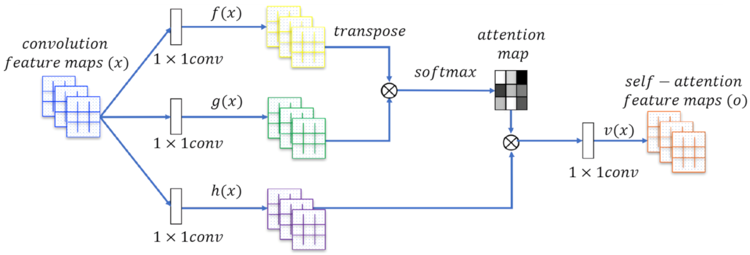
3.1.3. SAGAN (Self-Attention Generative Adversarial Networks)
3.2. Structure
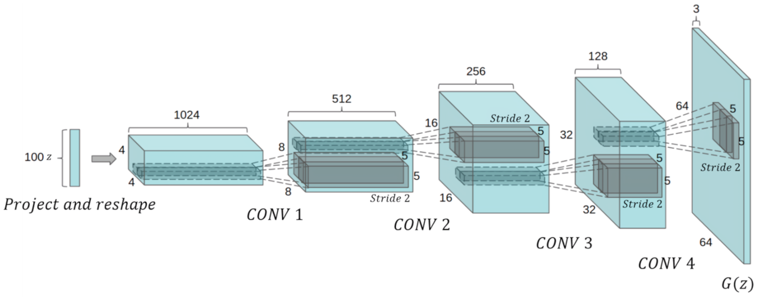
3.2.1. DCGAN (Deep Convolutional Generative Adversarial Networks)
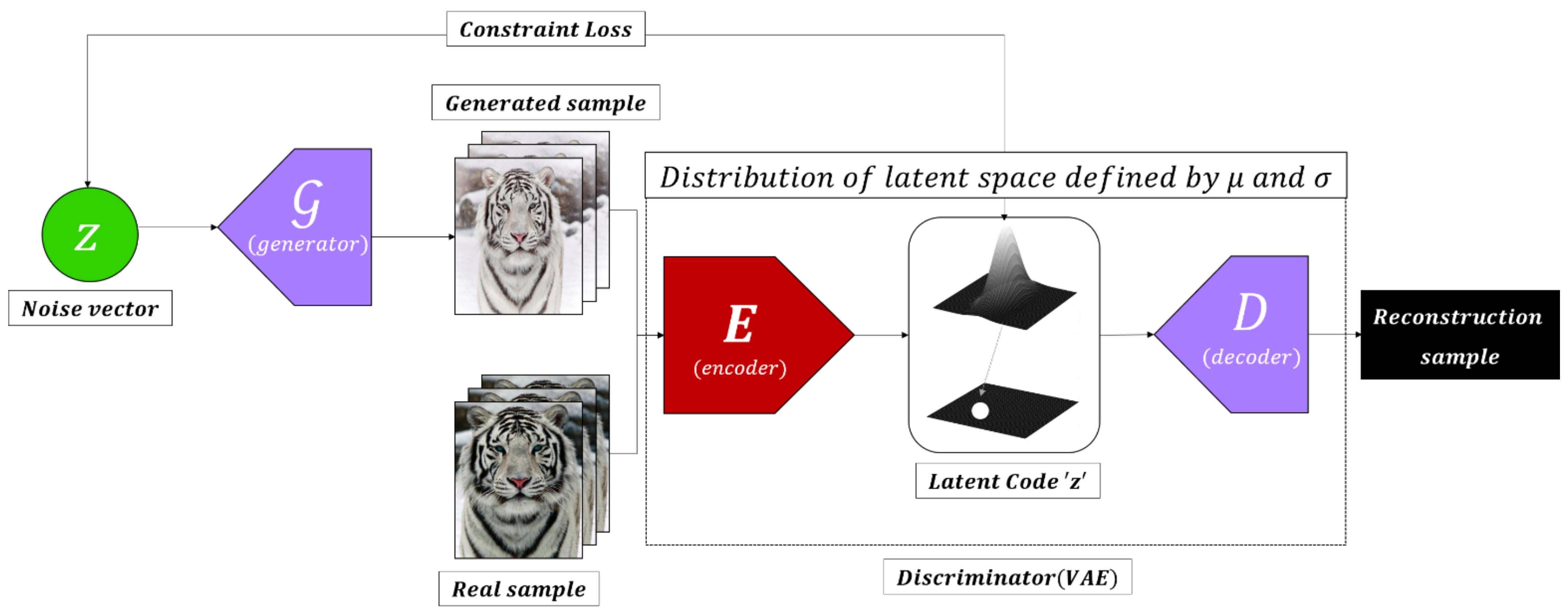
3.2.2. BEGAN (Boundary Equilibrium Generative Adversarial Networks)
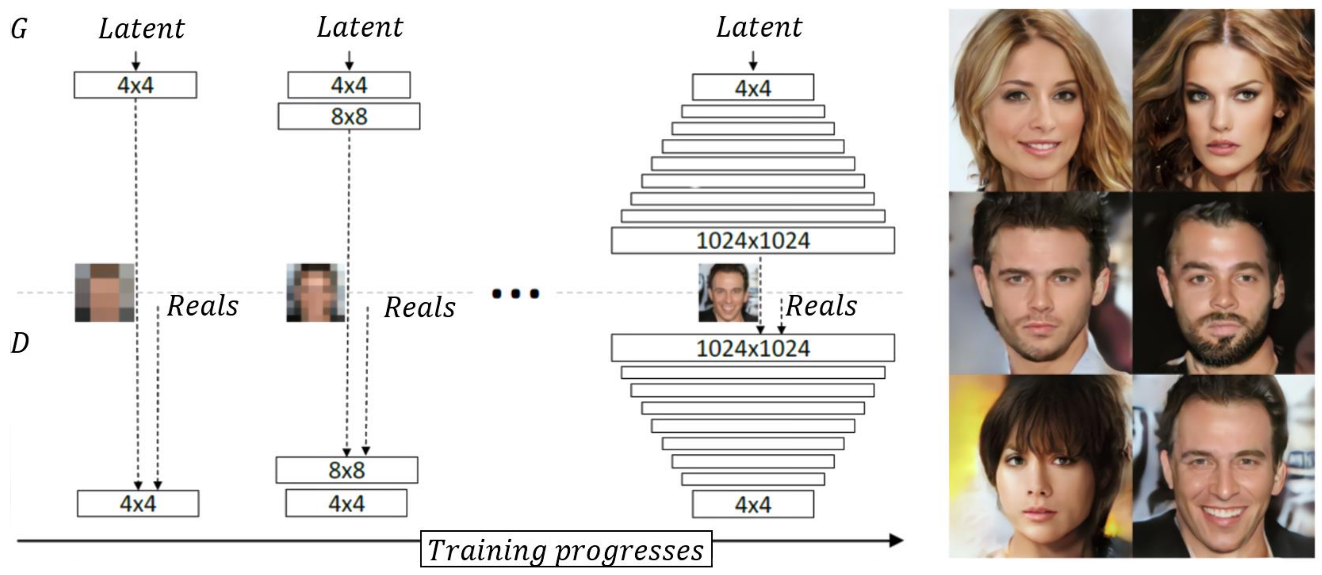
3.2.3. PGGAN (Progressive Growing of Generative Adversarial Networks)
3.3. Condition
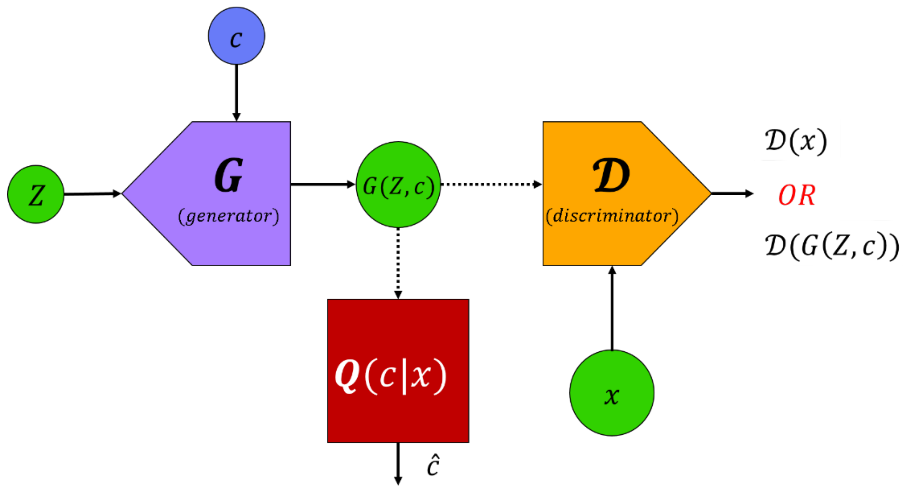
3.3.1. Info and Conditional GAN
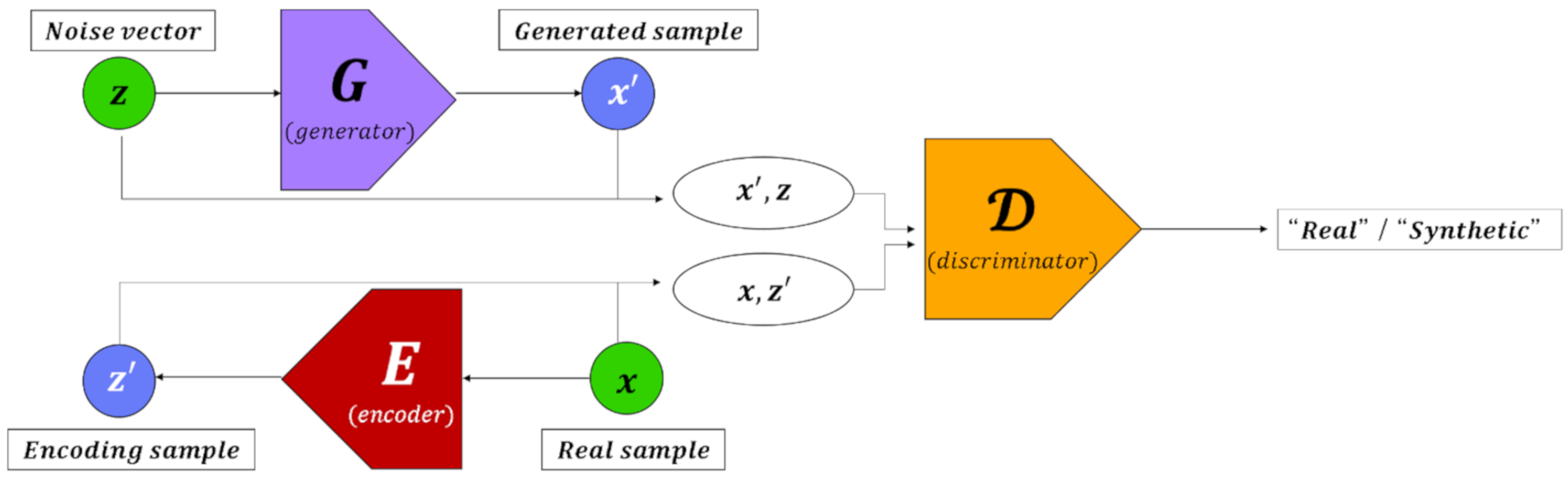
3.3.2. Inference Model Based on GAN
3.3.3. AAE (Adversarial Autoencoder)
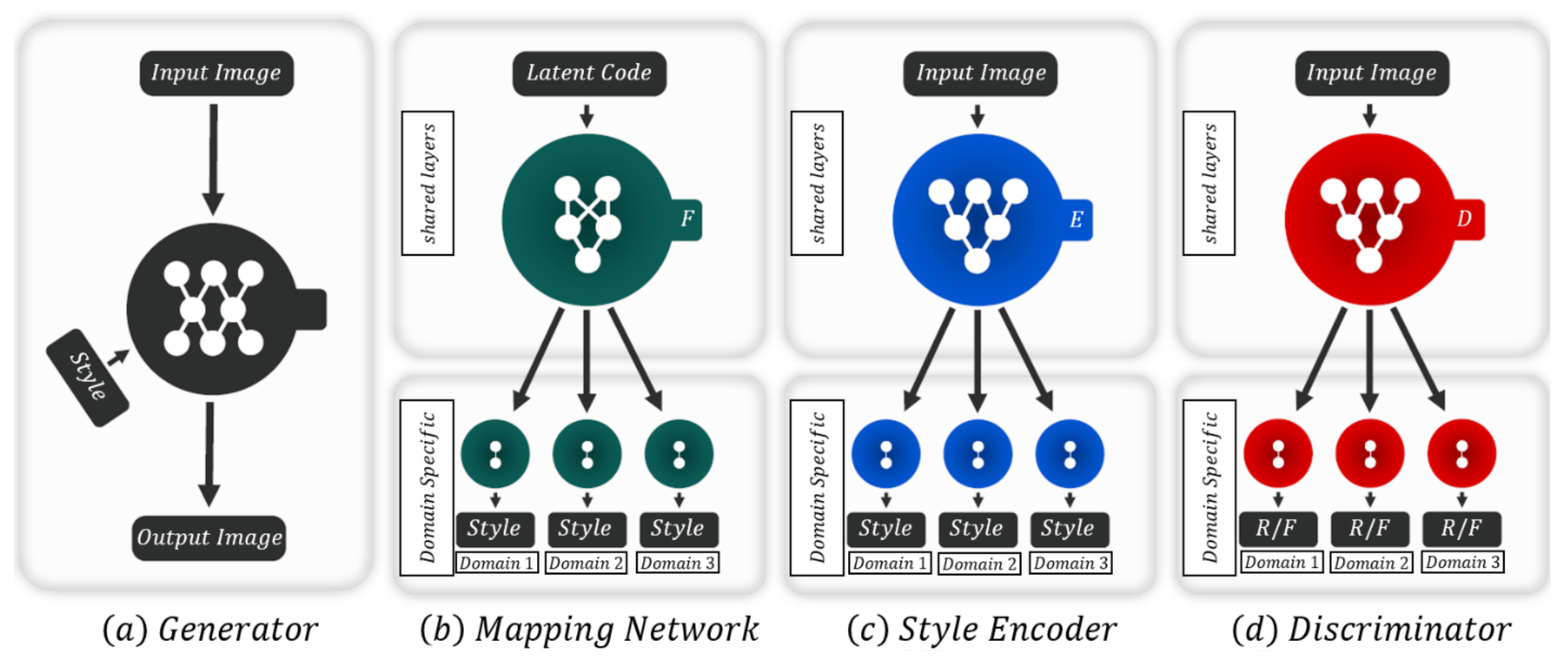
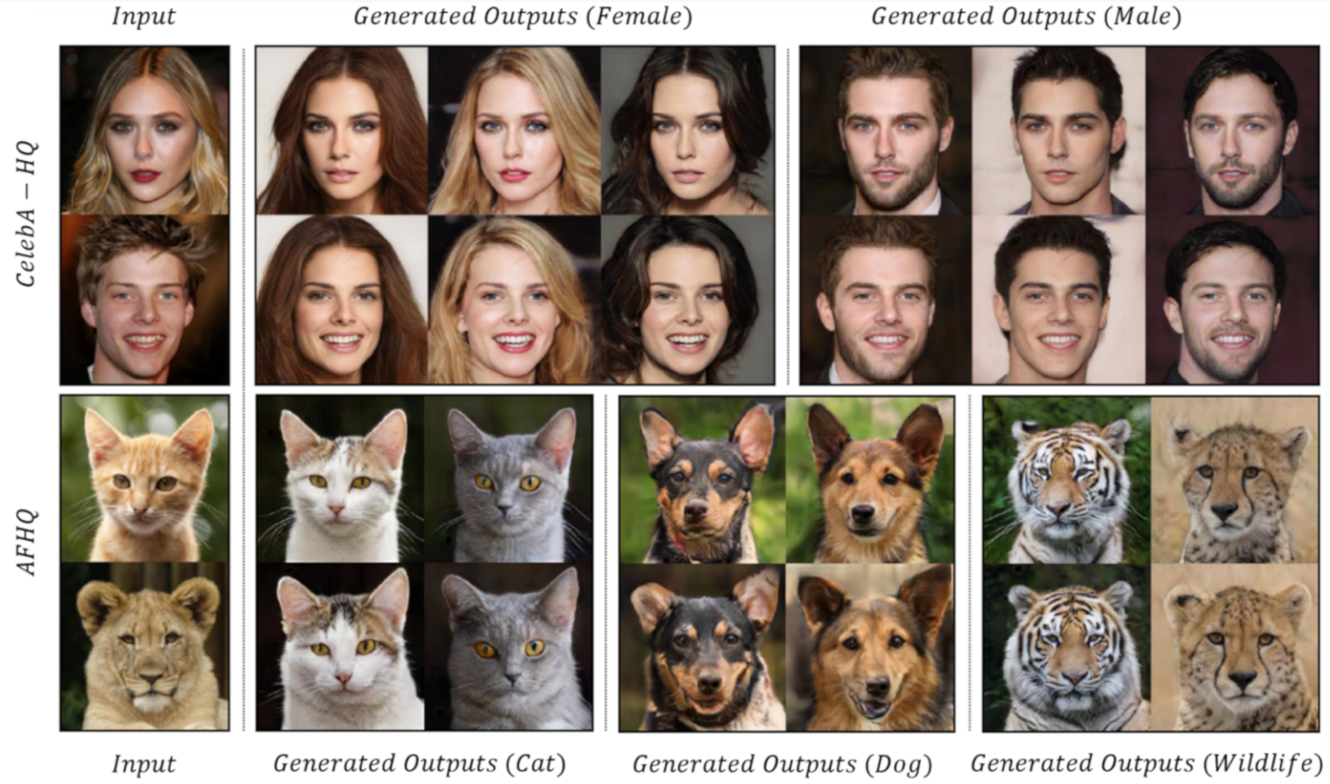
3.3.4. StarGAN
3.4. Mixing
3.4.1. BigGAN
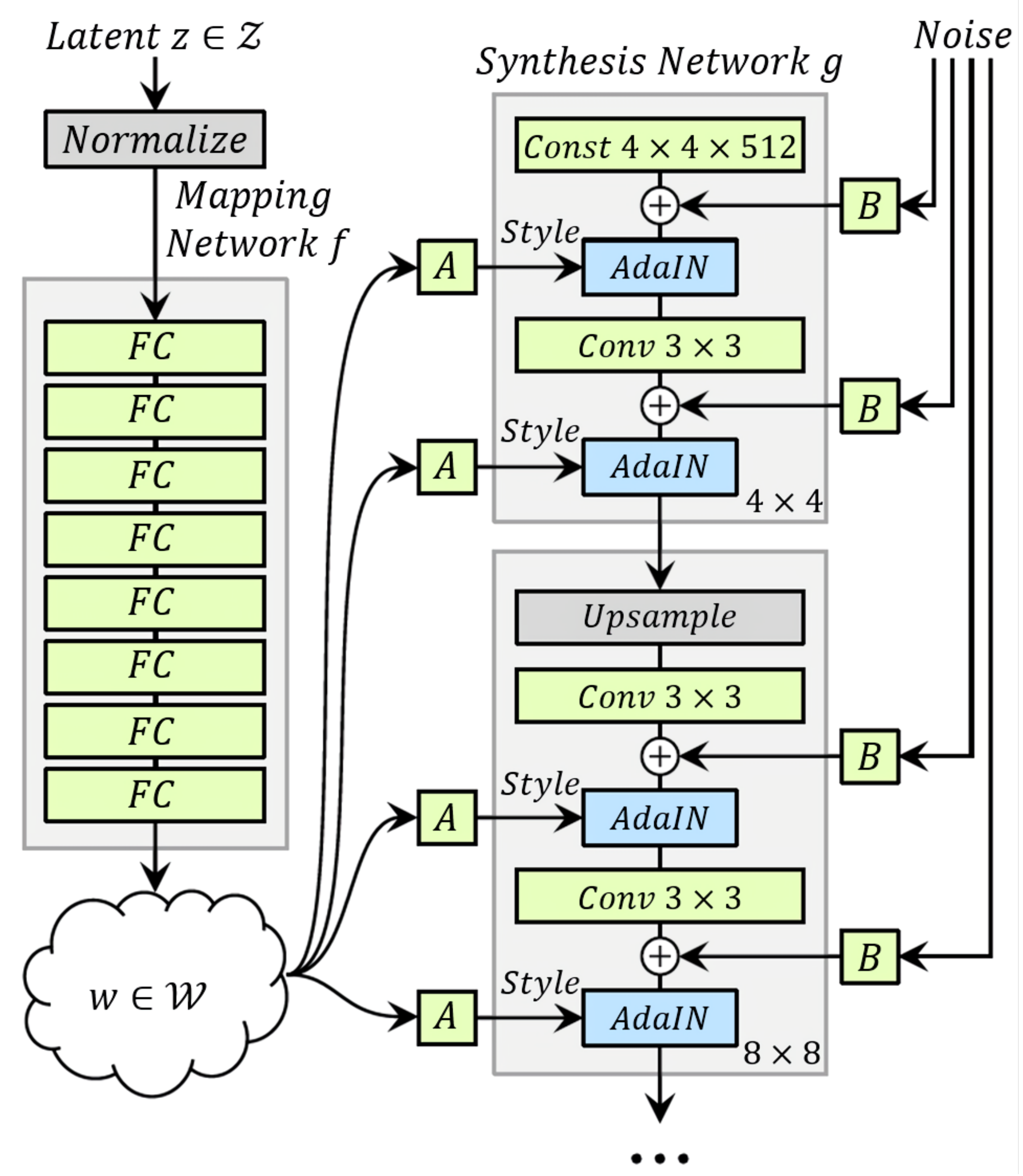
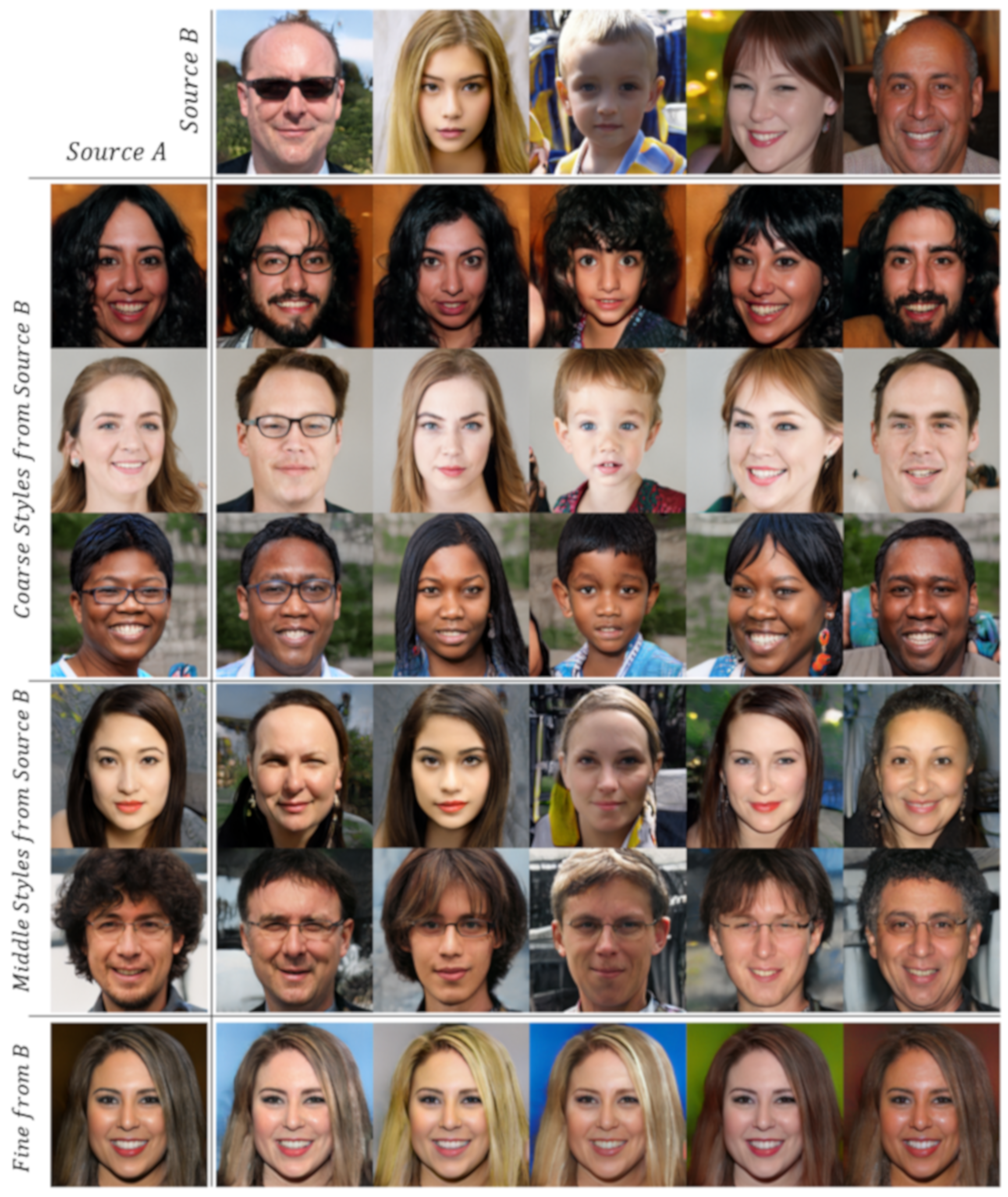
3.4.2. StyleGAN
4. Theory Analysis of GAN
4.1. Training Methods
4.2. Alternative Formulations
4.3. Disentangled Representation
4.4. Variants of GAN
4.5. Latent Space of GAN
5. Applications of GAN
5.1. Classification and Regression
5.2. Synthesis and Inpainting
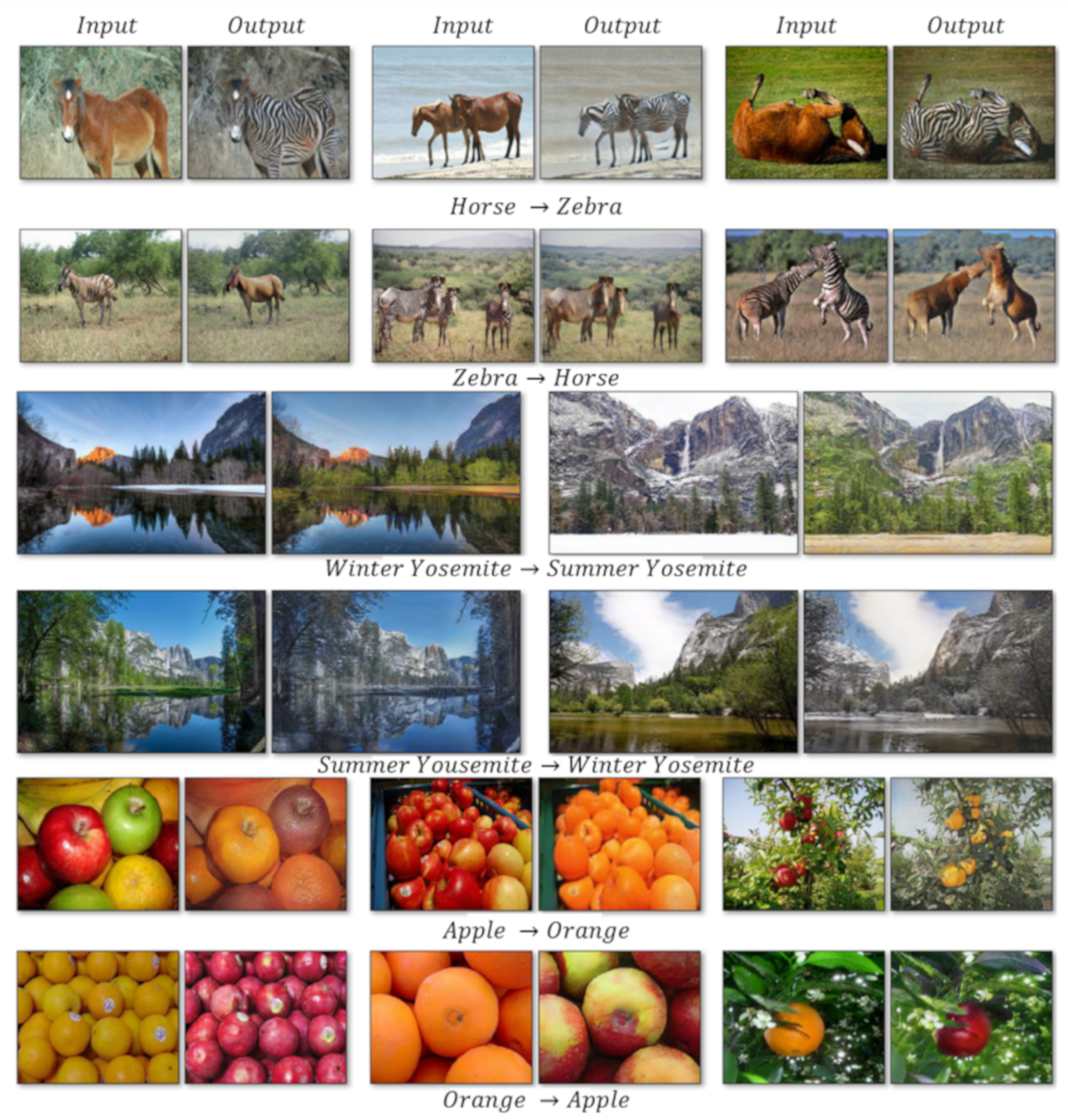
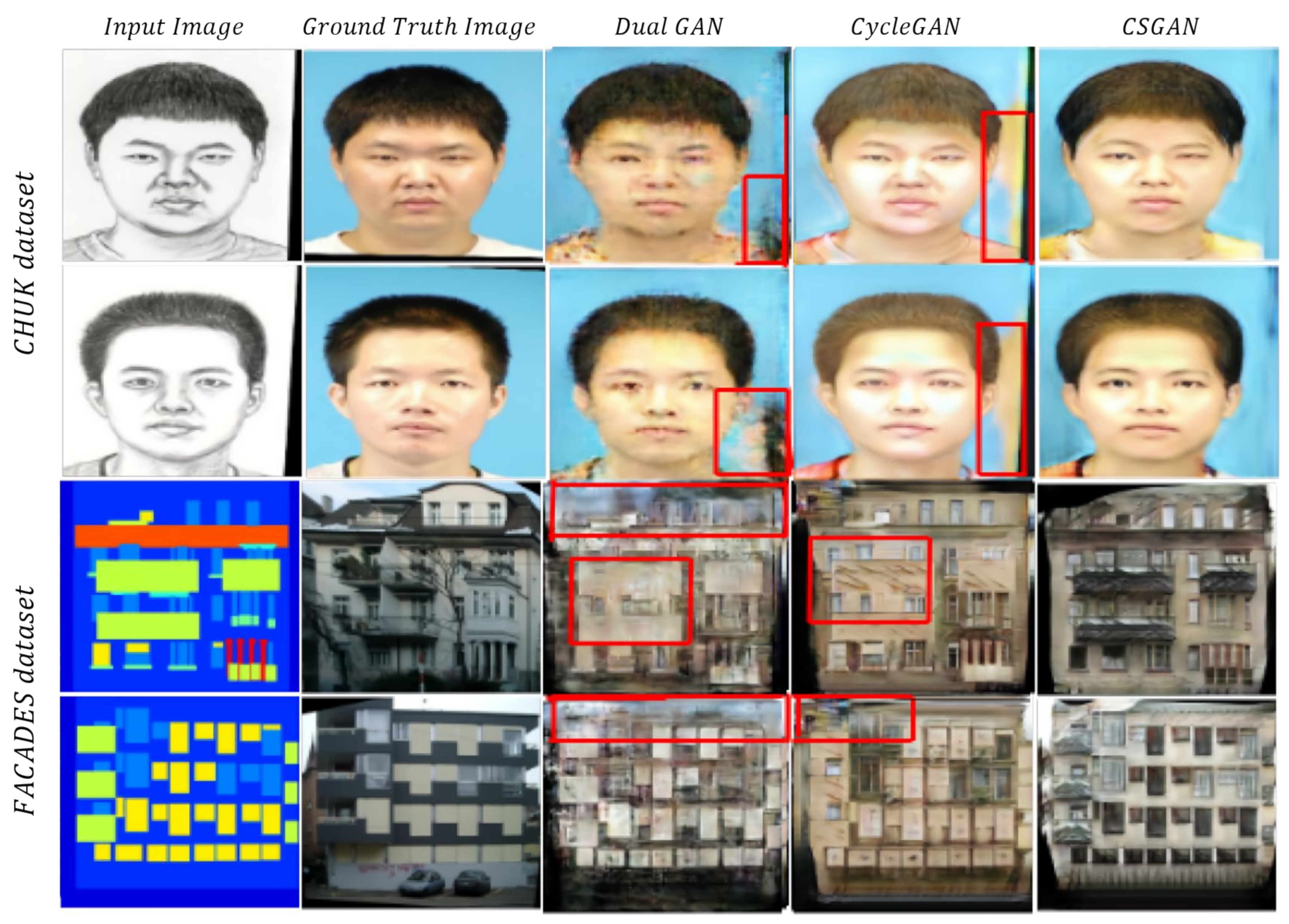
5.3. Image-to-Image Translation
5.4. Super-Resolution
5.5. Point Registration
6. Discussion
6.1. Mode Collapse
6.2. Training Instability
6.3. Evaluation Matrixs
6.4. Performance Comparisons
6.4.1. Qualitative Comparisons

| cGAN (Mirza et al., 2014) [33] | DCGAN (Radford et al., 2015) [20] | InfoGAN (Chen et al., 2016) [32] | BigGAN (Brock et al., 2018) [10] | |
| MNIST |  |  |  |  |
| DCGAN (Radford et al., 2015) [20] | WGAN (Arjovsky et al., 2017) [15] | WGAN-GP (Gulrajani et al., 2017) [17] | PGGAN (Karras et al., 2018) [8] | |
| LSUN Bedroom |  |  |  |  |
| DCGAN (Radford et al., 2015) [20] | SAGAN (Zhang et al., 2018) [9] | BigGAN (Brock et al., 2018) [10] | |
| ImageNet |  |  |  |
| ALI (Dumoulin et al., 2016) [36] | AVB (Mescheder et al., 2017) [41] | ALICE (Li et al., 2017) [38] | BEGANv3 (Park et al., 2020) [27] | |
| CelebA |  |  |  |  |
| PGGAN (Karras et al., 2017) [8] | StarGANv2 (Choi et al., 2019) [44] | MSG-StyleGAN (Karnewar et al., 2020) [95] | |
| CelebA-HQ |  |  |  |


6.4.2. Quantitative Comparisons
7. Conclusions
Author Contributions
Funding
Conflicts of Interest
References
- Yann, L.; Yoshua, B.; Geoffrey, H. Deep Learning. Nature 2015, 521, 436–444. [Google Scholar]
- Goodfellow, I.; Pouget-Abadie, J.; Mirza, M.; Xu, B.; Warde-Farley, D.; Ozair, S.; Bengio, Y. Generative adversarial nets. arXiv 2020, arXiv:1406.2661. Available online: https://arxiv.org/abs/1406.2661 (accessed on 21 April 2020).
- Vaswani, A.; Shazeer, N.; Parmar, N.; Uszkoreit, J.; Jones, L.; Gomez, A.N.; Polosukhin, I. Attention is all you need. arXiv 2020, arXiv:1706.03762. Available online: https://arxiv.org/abs/1706.03762 (accessed on 21 April 2020).
- Devlin, J.; Chang, M.W.; Lee, K.; Toutanova, K. Bert: Pre-Training of Deep Bidirectional Transformers for Language Understanding. arXiv 2020, arXiv:1810.04805. Available online: https://arxiv.org/abs/1810.04805 (accessed on 22 April 2020).
- Brown, T.B.; Mann, B.; Ryder, N.; Subbiah, M.; Kaplan, J.; Dhariwal, P.; Amodei, D. Language Models Are Few-Shot Learners. arXiv 2020, arXiv:2005.14165. Available online: https://arxiv.org/abs/2005.14165 (accessed on 22 August 2020).
- Payne, C. MuseNet. Available online: https://openai.com/blog/musenet (accessed on 23 April 2020).
- Yamamoto, R.; Song, E.; Kim, J.M. Parallel WaveGAN: A fast waveform generation model based on generative adversarial networks with multi-resolution spectrogram. In Proceedings of the ICASSP 2020–2020 IEEE International Conference on Acoustics, Speech and Signal Processing, Barcelona, Spain, 4–8 May 2020; IEEE: Piscataway, NJ, USA, 2020; pp. 6199–6203. [Google Scholar]
- Karras, T.; Aila, T.; Laine, S.; Lehtinen, J. Progressive Growing of Gans for Improved Quality, Stability, and Variation. arXiv 2020, arXiv:1710.10196. Available online: https://arxiv.org/abs/1710.10196 (accessed on 16 May 2020).
- Zhang, H.; Goodfellow, I.; Metaxas, D.; Odena, A. Self-Attention Generative Adversarial Networks. arXiv 2020, arXiv:1805.08318. Available online: https://arxiv.org/abs/1805.08318 (accessed on 17 May 2020).
- Brock, A.; Donahue, J.; Simonyan, K. Large Scale Gan Training for High Fidelity Natural Image Synthesis. arXiv 2020, arXiv:1809.11096. Available online: https://arxiv.org/abs/1809.11096 (accessed on 20 May 2020).
- Karras, T.; Laine, S.; Aila, T. A style-based generator architecture for generative adversarial networks. In Proceedings of the IEEE Conference on Computer Vision and Pattern Recognition, Long Beach, CA, USA, 16–20 June 2019; IEEE: Piscataway, NJ, USA, 2019; pp. 4401–4410. [Google Scholar]
- Nwankpa, C.; Ijomah, W.; Gachagan, A.; Marshall, S. Activation Functions: Comparison of Trends in Practice and Research for Deep Learning. arXiv 2020, arXiv:1811.03378. Available online: https://arxiv.org/abs/1811.03378 (accessed on 22 May 2020).
- LeCun, Y.; Touresky, D.; Hinton, G.; Sejnowski, T. A theoretical framework for back-propagation. In Proceedings of the 1988 Connectionist Models Summer School, San Mateo, CA, USA, 1 June 1988; Volume 1, pp. 21–28. [Google Scholar]
- Triola, M.F. Bayes’ Theorem. Available online: http://faculty.washington.edu/tamre/BayesTheorem.pdf (accessed on 10 January 2020).
- Arjovsky, M.; Chintala, S.; Bottou, L. Wasserstein Gan. arXiv 2020, arXiv:1701.07875. Available online: https://arxiv.org/abs/1701.07875 (accessed on 25 May 2020).
- Gouk, H.; Frank, E.; Pfahringer, B.; Cree, M. Regularisation of Neural Networks by Enforcing Lipschitz Continuity. arXiv 2020, arXiv:1804.04368. Available online: https://arxiv.org/abs/1804.04368 (accessed on 26 May 2020).
- Gulrajani, I.; Ahmed, F.; Arjovsky, M.; Dumoulin, V.; Courville, A.C. Improved training of wasserstein gans. In Proceedings of the Advances in Neural Information Processing Systems, Long Beach, CA, USA, 4–9 December 2017; Curran Associates Inc.: Red Hook, NY, USA, 2018; pp. 5767–5777. [Google Scholar]
- Ioffe, S.; Szegedy, C. Batch normalization: Accelerating Deep Network Training by Reducing Internal Covariate Shift. arXiv 2020, arXiv:1502.03167. Available online: https://arxiv.org/abs/1502.03167 (accessed on 28 May 2020).
- Krizhevsky, A.; Sutskever, I.; Hinton, G.E. Imagenet classification with deep convolutional neural networks. In Proceedings of the Advances in Neural Information Processing Systems, Lake Tahoe, NV, USA, 3–6 December 2012; Curran Associates Inc.: Red Hook, NY, USA, 2013; pp. 1097–1105. [Google Scholar]
- Radford, A.; Metz, L.; Chintala, S. Unsupervised Representation Learning with Deep Convolutional Generative Adversarial Networks. arXiv 2020, arXiv:1511.06434. Available online: https://arxiv.org/abs/1511.06434 (accessed on 29 May 2020).
- Kingma, D.P.; Welling, M. Auto-Encoding Variational Bayes. arXiv 2020, arXiv:1312.6114. Available online: https://arxiv.org/abs/1312.6114 (accessed on 1 June 2020).
- Kingma, D.P.; Ba, J. Adam: A Method for Stochastic Optimization. arXiv 2020, arXiv:1412.6980. Available online: https://arxiv.org/abs/1412.6980 (accessed on 2 June 2020).
- Yeh, R.; Chen, C.; Lim, T.Y.; Hasegawa-Johnson, M.; Do, M.N. Semantic Image Inpainting with Perceptual and Contextual Losses. arXiv 2020, arXiv:1607.07539. Available online: https://arxiv.org/abs/1607.07539 (accessed on 3 June 2020).
- Berthelot, D.; Schumm, T.; Metz, L. Began: Boundary Equilibrium Generative Adversarial Networks. arXiv 2020, arXiv:1703.10717. Available online: https://arxiv.org/abs/1703.10717 (accessed on 4 June 2020).
- Baldi, P. Autoencoders, unsupervised learning, and deep architectures. In Proceedings of the ICML Workshop on Unsupervised and Transfer Learning; Proceedings of Machine Learning Research, New York City, NY, USA, 19–24 June; 2016; pp. 37–49. [Google Scholar]
- Chang, C.C.; Hubert Lin, C.; Lee, C.R.; Juan, D.C.; Wei, W.; Chen, H.T. Escaping from collapsing modes in a constrained space. In Proceedings of the European Conference on Computer Vision, Munich, Germany, 8–14 September 2018; Springer: New York, NY, USA, 2019; pp. 204–219. [Google Scholar]
- Park, S.W.; Huh, J.H.; Kim, J.C. BEGAN v3: Avoiding Mode Collapse in GANs Using Variational Inference. Electronics 2020, 9, 688. [Google Scholar] [CrossRef]
- Clevert, D.A.; Unterthiner, T.; Hochreiter, S. Fast and Accurate Deep Network Learning by Exponential Linear Units (Elus). arXiv 2020, arXiv:1511.07289. Available online: https://arxiv.org/abs/1511.07289 (accessed on 5 June 2020).
- Maas, A.L.; Hannun, A.Y.; Ng, A.Y. Rectifier nonlinearities improve neural network acoustic models. Proc. ICML 2013, 30, 3. [Google Scholar]
- Pérez-Cruz, F. Kullback-Leibler divergence estimation of continuous distributions. In Proceedings of the 2008 IEEE International Symposium on Information Theory, Toronto, ON, Canada, 8 August 2008; IEEE: New York, NY, USA, 2008; pp. 1666–1670. [Google Scholar]
- Yu, F.; Seff, A.; Zhang, Y.; Song, S.; Funkhouser, T.; Xiao, J. Lsun: Construction of a Large-Scale Image Dataset Using Deep Learning with Humans in the Loop. arXiv 2020, arXiv:1506.03365. Available online: https://arxiv.org/abs/1506.03365 (accessed on 6 June 2020).
- Chen, X.; Duan, Y.; Houthooft, R.; Schulman, J.; Sutskever, I.; Abbeel, P. Infogan: Interpretable representation learning by information maximizing generative adversarial nets. In Proceedings of the Advances in Neural Information Processing Systems, Barcelona, Spain, 5–10 December 2016; Curran Associates Inc.: Red Hook, NY, USA, 2016; pp. 2172–2180. [Google Scholar]
- Mirza, M.; Osindero, S. Conditional Generative Adversarial Nets. arXiv 2020, arXiv:1411.1784. Available online: https://arxiv.org/abs/1411.1784 (accessed on 9 June 2020).
- Creswell, A.; Bharath, A.A. Inverting the Generator of a Generative Adversarial Network. IEEE Trans. Neural Networks Learn. Syst. 2019, 30, 1967–1974. [Google Scholar] [CrossRef] [PubMed]
- Lipton, Z.C.; Tripathi, S. Precise Recovery of Latent Vectors from Generative Adversarial Networks. arXiv 2020, arXiv:1702.04782. Available online: https://arxiv.org/abs/1702.04782 (accessed on 10 June 2020).
- Dumoulin, V.; Belghazi, I.; Poole, B.; Mastropietro, O.; Lamb, A.; Arjovsky, M.; Courville, A. Adversarially Learned Inference. arXiv 2020, arXiv:1606.00704. Available online: https://arxiv.org/abs/1606.00704 (accessed on 11 June 2020).
- Donahue, J.; Krähenbühl, P.; Darrell, T. Adversarial Feature Learning. arXiv 2020, arXiv:1605.09782. Available online: https://arxiv.org/abs/1605.09782 (accessed on 12 June 2020).
- Li, C.; Liu, H.; Chen, C.; Pu, Y.; Chen, L.; Henao, R.; Carin, L. Alice: Towards understanding adversarial learning for joint distribution matching. In Proceedings of the Advances in Neural Information Processing Systems, Long Beach, CA, USA, 4–9 December 2017; Curran Associates Inc.: Red Hook, NY, USA, 2017; pp. 5495–5503. [Google Scholar]
- Bengio, Y.; Yao, L.; Alain, G.; Vincent, P. Generalized Denoising Auto-Encoders as Generative Models. In Proceedings of the Advances in Neural Information Processing Systems, Lake Tahoe, NV, USA, 5–10 December 2013; Curran Associates Inc.: Red Hook, NY, USA, 2013; pp. 899–907. [Google Scholar]
- Makhzani, A.; Shlens, J.; Jaitly, N.; Goodfellow, I.; Frey, B. Adversarial Autoencoders. arXiv 2020, arXiv:1511.05644. Available online: https://arxiv.org/abs/1511.05644 (accessed on 15 June 2020).
- Mescheder, L.; Nowozin, S.; Geiger, A. Adversarial variational bayes: Unifying variational autoencoders and generative adversarial networks. In Proceedings of the 34th International Conference on Machine Learning, Sydney, Australia, 6–11 August 2017; Volume 70, pp. 2391–2400. [Google Scholar]
- Goodfellow, I. NIPS 2016 tutorial: Generative Adversarial Networks. arXiv 2020, arXiv:1701.00160. Available online: https://arxiv.org/abs/1701.00160 (accessed on 18 June 2020).
- Choi, Y.; Choi, M.; Kim, M.; Ha, J.W.; Kim, S.; Choo, J. Stargan: Unified generative adversarial networks for multi-domain image-to-image translation. In Proceedings of the IEEE Conference on Computer Vision and Pattern Recognition, Salt Lake City, UT, USA, 18–22 June 2018; Curran Associates Inc.: Red Hook, NY, USA, 2018; pp. 8789–8797. [Google Scholar]
- Choi, Y.; Uh, Y.; Yoo, J.; Ha, J.W. Stargan v2: Diverse image synthesis for multiple domains. In Proceedings of the IEEE/CVF Conference on Computer Vision and Pattern Recognition, Online, 14–19 June 2020; IEEE: New York, NY, USA, 2020; pp. 8188–8197. [Google Scholar]
- He, K.; Zhang, X.; Ren, S.; Sun, J. Identity Mappings in Deep Residual Networks. In Proceedings of the European Conference on Computer Vision, Amsterdam, The Netherlands, 8–16 October 2016; Springer: Cham, Switzerland, 2016; pp. 630–645. [Google Scholar]
- Liu, Z.; Luo, P.; Wang, X.; Tang, X. Deep Learning Face Attributes in the Wild. In Proceedings of the International Conference on Computer Vision, Araucano Park, Las Condes, Chile, 11–18 December 2015; IEEE Computer Society: Washington, DC, USA, 2015; pp. 3730–3738. [Google Scholar]
- Khan, M.H.; McDonagh, J.; Khan, S.; Shahabuddin, M.; Arora, A.; Khan, F.S.; Tzimiropoulos, G. AnimalWeb: A Large-Scale Hierarchical Dataset of Annotated Animal Faces. In Proceedings of the IEEE/CVF Conference on Computer Vision and Pattern Recognition, Online, 14–19 June 2020; IEEE: New York, NY, USA, 2020; pp. 6939–6948. [Google Scholar]
- Deng, J.; Dong, W.; Socher, R.; Li, L.J.; Li, K.; Fei-Fei, L. Imagenet: A large-scale hierarchical image database. In Proceedings of the 2009 IEEE Conference on Computer Vision and Pattern Recognition, Miami Beach, FL, USA, 20–26 June 2009; Curran Associates Inc.: Red Hook, NY, USA, 2009; pp. 248–255. [Google Scholar]
- Gatys, L.A.; Ecker, A.S.; Bethge, M. A neural Algorithm of Artistic Style. arXiv 2020, arXiv:1508.06576. Available online: https://arxiv.org/abs/1508.06576 (accessed on 1 July 2020). [CrossRef]
- Salimans, T.; Goodfellow, I.; Zaremba, W.; Cheung, V.; Radford, A.; Chen, X. Improved techniques for training gans. In Proceedings of the Advances in Neural Information Processing Systems, Barcelona, Spain, 5–10 December 2016; Curran Associates Inc.: Red Hook, NY, USA, 2016; pp. 2234–2242. [Google Scholar]
- Arjovsky, M.; Bottou, L. Towards Principled Methods for Training Generative Adversarial Networks. arXiv 2020, arXiv:1701.04862. Available online: https://arxiv.org/abs/1701.04862 (accessed on 2 July 2020).
- Long, J.; Shelhamer, E.; Darrell, T. Fully convolutional networks for semantic segmentation. In Proceedings of the IEEE Conference on Computer Vision and Pattern Recognition, Boston, MA, USA, 7–12 June 2015; IEEE: New York, NY, USA, 2016; pp. 3431–3440. [Google Scholar]
- Nair, V.; Hinton, G.E. Rectified linear units improve restricted boltzmann machines. In Proceedings of the 27th International Conference on Machine Learning, Haifa, Israel, 21–24 June 2010; Omnipress: Madison, WI, USA, 2010; pp. 807–814. [Google Scholar]
- Sønderby, C.K.; Caballero, J.; Theis, L.; Shi, W.; Huszár, F. Amortised Map Inference for Image Super-Resolution. arXiv 2020, arXiv:1610.04490. Available online: https://arxiv.org/abs/1610.04490 (accessed on 21 July 2020).
- Mescheder, L.; Nowozin, S.; Geiger, A. The Numerics of Gans. In Proceedings of the Advances in Neural Information Processing Systems, Long Beach, CA, USA, 4–9 December 2017; Curran Associates Inc.: Red Hook, NY, USA, 2017; pp. 1825–1835. [Google Scholar]
- Theis, L.; Oord, A.V.D.; Bethge, M. A Note on the Evaluation of Generative Models. arXiv 2020, arXiv:1511.01844. Available online: https://arxiv.org/abs/1511.01844 (accessed on 24 April 2020).
- Siddharth, N.; Paige, B.; Van de Meent, J.W.; Desmaison, A.; Goodman, N.; Kohli, P.; Torr, P. Learning disentangled representations with semi-supervised deep generative models. In Proceedings of the Advances in Neural Information Processing Systems, Long Beach, CA, USA, 4–9 December 2017; Curran Associates Inc.: Red Hook, NY, USA, 2017; pp. 5925–5935. [Google Scholar]
- Mikolov, T.; Chen, K.; Corrado, G.; Dean, J. Efficient Estimation of Word Representations in Vector Space. arXiv 2020, arXiv:1301.3781. Available online: https://arxiv.org/abs/1301.3781 (accessed on 18 May 2020).
- Gurumurthy, S.; Kiran Sarvadevabhatla, R.; Venkatesh Babu, R. Deligan: Generative adversarial networks for diverse and limited data. In Proceedings of the IEEE Conference on Computer Vision and Pattern Recognition, Honolulu, HI, USA, 21–26 July 2017; IEEE: New York, NY, USA, 2017; pp. 166–174. [Google Scholar]
- Ledig, C.; Theis, L.; Huszár, F.; Caballero, J.; Cunningham, A.; Acosta, A.; Shi, W. Photo-realistic single image super-resolution using a generative adversarial network. In Proceedings of the IEEE Conference on Computer Vision and Pattern Recognition, Honolulu, HI, USA, 21–26 July 2017; IEEE: New York, NY, USA, 2017; pp. 4681–4690. [Google Scholar]
- Yu, X.; Porikli, F. Ultra-resolving face images by discriminative generative networks. In Proceedings of the European Conference on Computer Vision, Amsterdam, The Netherlands, 8–16 October 2016; Springer: Cham, Switzerland, 2016; pp. 318–333. [Google Scholar]
- Yu, X.; Porikli, F. Hallucinating very low-resolution unaligned and noisy face images by transformative discriminative autoencoders. In Proceedings of the IEEE Conference on Computer Vision and Pattern Recognition, Honolulu, HI, USA, 21–26 July 2017; IEEE: New York, NY, USA, 2017; pp. 3760–3768. [Google Scholar]
- Shrivastava, A.; Pfister, T.; Tuzel, O.; Susskind, J.; Wang, W.; Webb, R. Learning from simulated and unsupervised images through adversarial training. In Proceedings of the IEEE Conference on Computer Vision and Pattern Recognition, Honolulu, HI, USA, 21–26 July 2017; IEEE: New York, NY, USA, 2017; pp. 2107–2116. [Google Scholar]
- Zhang, M.; Teck Ma, K.; Hwee Lim, J.; Zhao, Q.; Feng, J. Deep future gaze: Gaze anticipation on egocentric videos using adversarial networks. In Proceedings of the IEEE Conference on Computer Vision and Pattern Recognition, Honolulu, HI, USA, 21–26 July 2017; IEEE: New York, NY, USA, 2017; pp. 4372–4381. [Google Scholar]
- Bousmalis, K.; Silberman, N.; Dohan, D.; Erhan, D.; Krishnan, D. Unsupervised pixel-level domain adaptation with generative adversarial networks. In Proceedings of the IEEE Conference on Computer Vision and Pattern Recognition, Honolulu, HI, USA, 21–26 July 2017; IEEE: New York, NY, USA, 2017; pp. 3722–3731. [Google Scholar]
- Liu, M.Y.; Tuzel, O. Coupled generative adversarial networks. In Proceedings of the Advances in Neural Information Processing Systems, Barcelona, Spain, 5–10 December 2016; Curran Associates Inc.: Red Hook, NY, USA, 2016; pp. 469–477. [Google Scholar]
- Denton, E.L.; Chintala, S.; Fergus, R. Deep generative image models using a laplacian pyramid of adversarial networks. In Proceedings of the Advances in Neural Information Processing Systems, Barcelona, Spain, 5–10 December 2016; Curran Associates Inc.: Red Hook, NY, USA, 2016; pp. 1486–1494. [Google Scholar]
- Huang, X.; Li, Y.; Poursaeed, O.; Hopcroft, J.; Belongie, S. Stacked generative adversarial networks. In Proceedings of the IEEE Conference on Computer Vision and Pattern Recognition, Honolulu, Hawaii, USA, 21–26 July 2017; IEEE: New York, NY, USA, 2017; pp. 5077–5086. [Google Scholar]
- Reed, S.; Akata, Z.; Yan, X.; Logeswaran, L.; Schiele, B.; Lee, H. Generative Adversarial Text to Image Synthesis. arXiv 2020, arXiv:1605.05396. Available online: https://arxiv.org/abs/1605.05396 (accessed on 23 May 2020).
- Reed, S.E.; Akata, Z.; Mohan, S.; Tenka, S.; Schiele, B.; Lee, H. Learning what and where to draw. In Proceedings of the Advances in Neural Information Processing Systems, Barcelona, Spain, 5–10 December 2016; Curran Associates Inc.: Red Hook, NY, USA, 2016; pp. 217–225. [Google Scholar]
- Zhu, J.Y.; Krähenbühl, P.; Shechtman, E.; Efros, A.A. Generative visual manipulation on the natural image manifold. In Proceedings of the European Conference on Computer Vision, Amsterdam, The Netherlands, 8–16 October 2016; Springer: Cham, Switzerland, 2016; pp. 597–613. [Google Scholar]
- Brock, A.; Lim, T.; Ritchie, J.M.; Weston, N. Neural Photo Editing with Introspective Adversarial Networks. arXiv 2020, arXiv:1609.07093. Available online: https://arxiv.org/abs/1609.07093 (accessed on 27 May 2020).
- Yurt, M.; Dar, S.U.; Erdem, A.; Erdem, E.; Oguz, K.K.; Çukur, T. mustGAN: Multi-Stream Generative Adversarial Networks for MR Image Synthesis. Med. Image Anal. 2021, 70, 101944. [Google Scholar] [CrossRef]
- Cai, W.; Wei, Z. PiiGAN: Generative Adversarial Networks for Pluralistic Image Inpainting. IEEE Access 2020, 8, 48451–48463. [Google Scholar] [CrossRef]
- Isola, P.; Zhu, J.-Y.; Zhou, T.; Efros, A.A. Image-to-Image Translation with Conditional Adversarial Networks. In Proceedings of the IEEE Conference on Computer Vision and Pattern Recognition, Honolulu, HI, USA, 21–26 July 2017; pp. 5967–5976. [Google Scholar]
- Zhu, J.Y.; Park, T.; Isola, P.; Efros, A.A. Unpaired image-to-image translation using cycle-consistent adversarial networks. In Proceedings of the IEEE International Conference on Computer Vision, Venice, Italy, 22–29 October 2017; IEEE: New York, NY, USA, 2017; pp. 2223–2232. [Google Scholar]
- Babu, K.K.; Dubey, S.R. CSGAN: Cyclic-Synthesized Generative Adversarial Networks for image-to-image transformation. Expert Syst. Appl. 2021, 169, 114431. [Google Scholar] [CrossRef]
- Wang, X.; Tang, X. Face Photo-Sketch Synthesis and Recognition. IEEE Trans. Pattern Anal. Mach. Intell. 2009, 31, 1955–1967. [Google Scholar] [CrossRef]
- Tyleček, R.; Šára, R. Spatial pattern templates for recognition of objects with regular structure. In Proceedings of the German Conference on Pattern Recognition, Saarbrücken, Germany, 3–6 September 2013; Springer: Cham, Switzerland, 2013; pp. 364–374. [Google Scholar]
- Yi, Z.; Zhang, H.; Tan, P.; Gong, M. Dualgan: Unsupervised dual learning for image-to-image translation. In Proceedings of the IEEE International Conference on Computer Vision, Venice, Italy, 22–29 October 2017; IEEE: New York, NY, USA, 2017; pp. 2849–2857. [Google Scholar]
- Scott, E. Artist, Creative AI, Scott’s Blog. Available online: http://www.scott-eaton.com/ (accessed on 10 March 2020).
- Kim, T.; Park, E.; Lee, H.; Moon, Y.-J.; Bae, S.-H.; Lim, D.; Jang, S.; Kim, L.; Cho, I.-H.; Choi, M.; et al. Solar farside magnetograms from deep learning analysis of STEREO/EUVI data. Nat. Astron. 2019, 3, 397–400. [Google Scholar] [CrossRef]
- He, K.; Zhang, X.; Ren, S.; Sun, J. Deep residual learning for image recognition. In Proceedings of the IEEE Conference on Computer Vision and Pattern Recognition, Las Vegas, NV, USA,, 26 June–1 July 2016; Curran Associates Inc.: Red Hook, NY, USA, 2016; pp. 770–778. [Google Scholar]
- Simonyan, K.; Zisserman, A. Very Deep Convolutional Networks for Large-Scale Image Recognition. arXiv 2020, arXiv:1409.1556. Available online: https://arxiv.org/abs/1409.1556 (accessed on 7 June 2020).
- Mahapatra, D.; Ge, Z. Training data independent image registration using generative adversarial networks and domain adaptation. Pattern Recognit. 2020, 100, 107109. [Google Scholar] [CrossRef]
- Arora, S.; Ge, R.; Liang, Y.; Ma, T.; Zhang, Y. Generalization and equilibrium in generative adversarial nets (gans). In Proceedings of the 34th International Conference on Machine Learning, Sydney, Australia, 6–11 August 2017; Volume 70, pp. 224–232. [Google Scholar]
- Zhao, J.; Mathieu, M.; LeCun, Y. Energy-Based Generative Adversarial Network. arXiv 2020, arXiv:1609.03126. Available online: https://arxiv.org/abs/1609.03126 (accessed on 8 June 2020).
- Metz, L.; Poole, B.; Pfau, D.; Sohl-Dickstein, J. Unrolled Generative Adversarial Networks. arXiv 2020, arXiv:1611.02163. Available online: https://arxiv.org/abs/1611.02163 (accessed on 13 June 2020).
- Lee, J.D.; Simchowitz, M.; Jordan, M.I.; Recht, B. Gradient descent only converges to minimizers. In Proceedings of the Conference on Learning Theory, New York, NY, USA, 23–26 June 2016; pp. 1246–1257. [Google Scholar]
- Pemantle, R. Nonconvergence to Unstable Points in Urn Models and Stochastic Approximations. Ann. Probab. 1990, 18, 698–712. [Google Scholar] [CrossRef]
- Barratt, S.; Sharma, R. A Note on the Inception Score. arXiv 2020, arXiv:1801.01973. Available online: https://arxiv.org/abs/1801.01973 (accessed on 14 June 2020).
- Heusel, M.; Ramsauer, H.; Unterthiner, T.; Nessler, B.; Hochreiter, S. Gans trained by a two time-scale update rule converge to a local nash equilibrium. In Proceedings of the Advances in Neural Information Processing Systems, Long Beach, CA, USA, 4–9 December 2017; Curran Associates Inc.: Red Hook, NY, USA, 2017; pp. 6626–6637. [Google Scholar]
- Szegedy, C.; Vanhoucke, V.; Ioffe, S.; Shlens, J.; Wojna, Z. Rethinking the inception architecture for computer vision. In Proceedings of the IEEE Conference on Computer Vision and Pattern Recognition, Las Vegas, NV, USA, 26 June–1 July 2016; Curran Associates Inc.: Red Hook, NY, USA, 2016; pp. 2818–2826. [Google Scholar]
- Sajjadi, M.S.; Bachem, O.; Lucic, M.; Bousquet, O.; Gelly, S. Assessing generative models via precision and recall. In Proceedings of the Advances in Neural Information Processing Systems, Montreal, QC, Canada, 3–8 December 2018; Curran Associates Inc.: Red Hook, NY, USA, 2018; pp. 5228–5237. [Google Scholar]
- Karnewar, A.; Wang, O. Msg-gan: Multi-scale gradients for generative adversarial networks. In Proceedings of the IEEE/CVF Conference on Computer Vision and Pattern Recognition, Online, 14–19 June 2020; IEEE: New York, NY, USA, 2020; pp. 7799–7808. [Google Scholar]
- Zhao, Y.; Li, C.; Yu, P.; Gao, J.; Chen, C. Feature Quantization Improves GAN Training. arXiv 2020, arXiv:2004.02088. Available online: https://arxiv.org/abs/2004.02088 (accessed on 15 August 2020).
- Kynkäänniemi, T.; Karras, T.; Laine, S.; Lehtinen, J.; Aila, T. Improved Precision and Recall Metric for Assessing Generative models. arXiv 2020, arXiv:1904.06991. Available online: https://arxiv.org/abs/1904.06991 (accessed on 16 June 2020).
- Karras, T.; Aittala, M.; Hellsten, J.; Laine, S.; Lehtinen, J.; Aila, T. Training Generative Adversarial Networks with Limited Data. arXiv 2020, arXiv:2006.06676. Available online: https://arxiv.org/abs/2006.06676 (accessed on 7 November 2020).
- Zhang, H.; Zhang, Z.; Odena, A.; Lee, H. Consistency Regularization for Generative Adversarial Networks. arXiv 2020, arXiv:1910.12027. Available online: https://arxiv.org/abs/1910.12027 (accessed on 17 June 2020).
- Zhao, S.; Liu, Z.; Lin, J.; Zhu, J.Y.; Han, S. Differentiable Augustmentation for Data-Efficient Gan Training. arXiv 2020, arXiv:2006.10738. Available online: https://arxiv.org/abs/2006.10738 (accessed on 7 January 2021).
- Tang, S. Lessons Learned from the Training of GANs on Artificial Datasets. IEEE Access 2020, 8, 165044–165055. [Google Scholar] [CrossRef]
- Patel, P.; Kumari, N.; Singh, M.; Krishnamurthy, B. LT-GAN: Self-Supervised GAN with Latent Transformation Detection. In Proceedings of the IEEE/CVF Winter Conference on Applications of Computer Vision, Waikoloa, HI, USA, 5–9 January 2021; pp. 3189–3198. [Google Scholar]
- Terjék, D. Adversarial Lipschitz Regularization. arXiv 2020, arXiv:1907.05681. Available online: https://arxiv.org/abs/1907.05681 (accessed on 3 July 2020).
- Wu, J.; Huang, Z.; Acharya, D.; Li, W.; Thoma, J.; Paudel, D.P.; Gool, L.V. Sliced wasserstein generative models. In Proceedings of the IEEE/CVF Conference on Computer Vision and Pattern Recognition, Long Beach, CA, USA, 16–20 June 2019; IEEE: Piscataway, NJ, USA, 2019; pp. 3713–3722. [Google Scholar]
- Zhang, H.; Xu, T.; Li, H.; Zhang, S.; Wang, X.; Huang, X.; Metaxas, D.N. Stackgan++: Realistic image synthesis with stacked generative adversarial networks. IEEE Trans. Pattern Anal. Mach. Intell. 2018, 41, 1947–1962. [Google Scholar] [CrossRef]
- Karras, T.; Laine, S.; Aittala, M.; Hellsten, J.; Lehtinen, J.; Aila, T. Analyzing and improving the image quality of stylegan. In Proceedings of the IEEE/CVF Conference on Computer Vision and Pattern Recognition, Online, 14–19 June 2020; IEEE: New York, NY, USA, 2020; pp. 8110–8119. [Google Scholar]
- Suh, S.; Lee, H.; Lukowicz, P.; Lee, Y.O. CEGAN: Classification Enhancement Generative Adversarial Networks for unraveling data imbalance problems. Neural. Networks 2021, 133, 69–86. [Google Scholar] [CrossRef] [PubMed]
- Prisma Labs, Prisma Photo Editor. Available online: http://www.prisma-ai.com/index.html (accessed on 12 May 2020).
- Zhavoronkov, A.; Zagribelnyy, B.; Zhebrak, A.; Aladinskiy, V.; Terentiev, V.; Vanhaelen, Q.; Bishop, M. Potential Non-Covalent SARS-CoV-2 3C-Like Protease Inhibitors Designed Using Generative Deep Learning Approaches and Reviewed by Human Medicinal Chemist in Virtual Reality. ChemRxiv 2020. [Google Scholar] [CrossRef]
- Sutton, R.S.; Barto, A.G. Reinforcement Learning: An Introduction; MIT Press: Cambridge, MA, USA, 2018. [Google Scholar]
- Goertzel, B. Artificial General Intelligence; Springer: Berlin/Heidelberg, Germany, 2007; Volume 2. [Google Scholar]


| Dataset | Model | IS (↑) | |
|---|---|---|---|
| CIFAR-10 (6464) | ALI | (Dumoulin et al., 2016) [36] | 5.34 |
| BEGAN | (Berthelot et al., 2017) [24] | 5.62 | |
| WGAN-GP | (Gulrajani et al., 2017) [17] | 7.86 | |
| PGGAN | (Karras et al., 2018) [8] | 8.80 | |
| BigGAN | (Brock et al., 2018) [10] | 9.22 |
| Dataset | Model | FID (↓) | |
|---|---|---|---|
| CIFAR-10 (6464) | StyleGAN2+ADA+Tuning | (Karras et al., 2020) [98] | 2.92 |
| CR-BigGAN+DiffAugment | (Zhao et al., 2020) [100] | 4.30 | |
| BigGAN+DiffAugment | 4.61 | ||
| StyleGAN2+DiffAugment | 5.79 | ||
| BigGAN+MIX | (Tang et al., 2020) [101] | 8.17 | |
| BigGAN+CR+LT | (Patel et al., 2020) [102] | 9.80 | |
| WGAN-ALP | (Terjek et al., 2019) [103] | 12.96 | |
| BigGAN | (Brock et al., 2018) [10] | 14.73 | |
| WGAN-GP | (Gulrajani et al., 2017) [17] | 29.30 |
| Dataset | Model | FID (↓) | ||
|---|---|---|---|---|
| 100% Training Data | 20% Training Data | 10% Training Data | ||
| CIFAR-10 (6464) | StyleGAN2+DiffAugment [100] | 5.79 | 12.15 | 14.50 |
| CR-BigGAN+DiffAugment [100] | 4.30 | 12.84 | 18.70 | |
| BigGAN+DiffAugment [100] | 4.61 | 14.04 | 22.40 | |
| Dataset | Model | IS (↑) | FID (↓) | |
|---|---|---|---|---|
| ImageNet (128128) | BigGAN-deep | (Brock et al., 2019) [10] | 124.5 | 5.7 |
| CR-BigGAN | (Zhang et al., 2020) [99] | - | 6.7 | |
| BigGAN+DiffAugment | (Zhao et al., 2020) [100] | 100.8 | 6.8 | |
| BigGAN | (Brock et al., 2019) [10] | 98.8 | 8.7 |
| Dataset | Model | Category | FID (↓) | |
|---|---|---|---|---|
| LSUN (256 256) | StyleGAN | (Karras et al., 2019) [11] | Bedroom | 2.65 |
| PG-SWGAN | (Wu et al., 2019) [104] | 8.00 | ||
| PGGAN | (Karras et al., 2018) [8] | 8.34 | ||
| StackGAN2 | (Zhang et al., 2017) [105] | 35.61 |
| Dataset | Model | Category | FID (↓) | |
|---|---|---|---|---|
| LSUN (256256) | StyleGAN2 | (Karras et al., 2020) [106] | Churches | 3.86 |
| StyleGAN | (Karras et al., 2019) [11] | 4.21 | ||
| MSG-StyleGAN | (Karras et al., 2018) [95] | 5.20 | ||
| PGGAN | (Zhang et al., 2018) [8] | 6.42 |
| Dataset | Model | Category | Image Size | FID (↓) |
|---|---|---|---|---|
| LSUN | StyleGAN2 [106] | Car | 256256 | 2.32 |
| Cat | 6.93 | |||
| Churches | 3.86 | |||
| Horse | 3.43 | |||
| Car | 512384 | 2.32 |
| Dataset | Model | FID (↓) | |
|---|---|---|---|
| CelebA-HQ (1024 1024) | StyleGAN | (Karras et al., 2019) [11] | 5.06 |
| PG-SWGAN | (Wu et al., 2019) [104] | 5.50 | |
| MSG-StyleGAN | (Karnewar et al., 2020) [95] | 6.37 | |
| PGGAN | (Karras et al., 2018) [8] | 7.30 |
| Dataset | Model | FID (↓) | |
|---|---|---|---|
| FFHQ (1024 1024) | StyleGAN2 | (Karras et al., 2020) [106] | 2.84 |
| StyleGAN+No Instance Normalization | (Kynkaanniemi et al., 2019) [97] | 4.16 | |
| StyleGAN | (Karras et al., 2019) [11] | 4.43 | |
| MSG-StyleGAN | (Karnewar et al., 2020) [95] | 5.80 | |
| PGGAN | (Karras et al., 2018) [8] | 8.40 |
| Dataset | Model | FID (↓) | |
|---|---|---|---|
| CIFAR-10 (64 64) | StyleGAN2+ADA+Tuning | (Karras et al., 2020) [98] | 2.92 |
| ImageNet (128 128) | BigGAN-deep | (Brock et al., 2019) [10] | 5.70 |
| LSUN Bedroom (256 256) | StyleGAN | (Karras et al., 2019) [11] | 2.65 |
| LSUN Churches (256 256) | StyleGAN2 | (Karras et al., 2020) [106] | 3.86 |
| CelebA-HQ (1024 1024) | StyleGAN | (Karras et al., 2019) [11] | 5.06 |
| FFHQ (1024 1024) | StyleGAN2 | (Karras et al., 2020) [106] | 2.84 |
Publisher’s Note: MDPI stays neutral with regard to jurisdictional claims in published maps and institutional affiliations. |
© 2021 by the authors. Licensee MDPI, Basel, Switzerland. This article is an open access article distributed under the terms and conditions of the Creative Commons Attribution (CC BY) license (https://creativecommons.org/licenses/by/4.0/).
Share and Cite
Park, S.-W.; Ko, J.-S.; Huh, J.-H.; Kim, J.-C. Review on Generative Adversarial Networks: Focusing on Computer Vision and Its Applications. Electronics 2021, 10, 1216. https://doi.org/10.3390/electronics10101216
Park S-W, Ko J-S, Huh J-H, Kim J-C. Review on Generative Adversarial Networks: Focusing on Computer Vision and Its Applications. Electronics. 2021; 10(10):1216. https://doi.org/10.3390/electronics10101216
Chicago/Turabian StylePark, Sung-Wook, Jae-Sub Ko, Jun-Ho Huh, and Jong-Chan Kim. 2021. "Review on Generative Adversarial Networks: Focusing on Computer Vision and Its Applications" Electronics 10, no. 10: 1216. https://doi.org/10.3390/electronics10101216
APA StylePark, S.-W., Ko, J.-S., Huh, J.-H., & Kim, J.-C. (2021). Review on Generative Adversarial Networks: Focusing on Computer Vision and Its Applications. Electronics, 10(10), 1216. https://doi.org/10.3390/electronics10101216