
Estimating Software Development Efforts Using a Random Forest-Based Stacked Ensemble Approach


Abstract
1. Introduction
- ⮚
- Inception phase
- ⮚
- Requirement phase
- ⮚
- Design phase
- ⮚
- Construction phase
- ⮚
- Testing phase
- ⮚
- Deployment phase
- ⮚
- Maintenance phase
- Averaging: It is performed by taking the average of prediction from a single model.
- Weighted Average: It is calculated by applying different weights to different single models, based on their prediction and finally taking the average weighted predictions.
- Bagging: It is otherwise called Bootstrap aggregation, a kind of sampling technique. Multiple samples are considered from the original dataset and similar to random forest techniques.
- Boosting: It uses a sequential method to reduce the bias. Various boosting algorithms used are XGBoost (eXtreme Gradient Boosting), GBM (Gradient Boosting Machine), AdaBoost (Adaptive Boosting).
- Stacking: Stacking does prediction from multiple models and builds a novel model.
2. Related Work
3. Mathematical Modeling
3.1. Software Effort Estimation Evaluation Metrics
3.1.1. Mean Absolute Error (MAE)
3.1.2. Root Mean Square Error (RMSE)
3.1.3. R-Squared
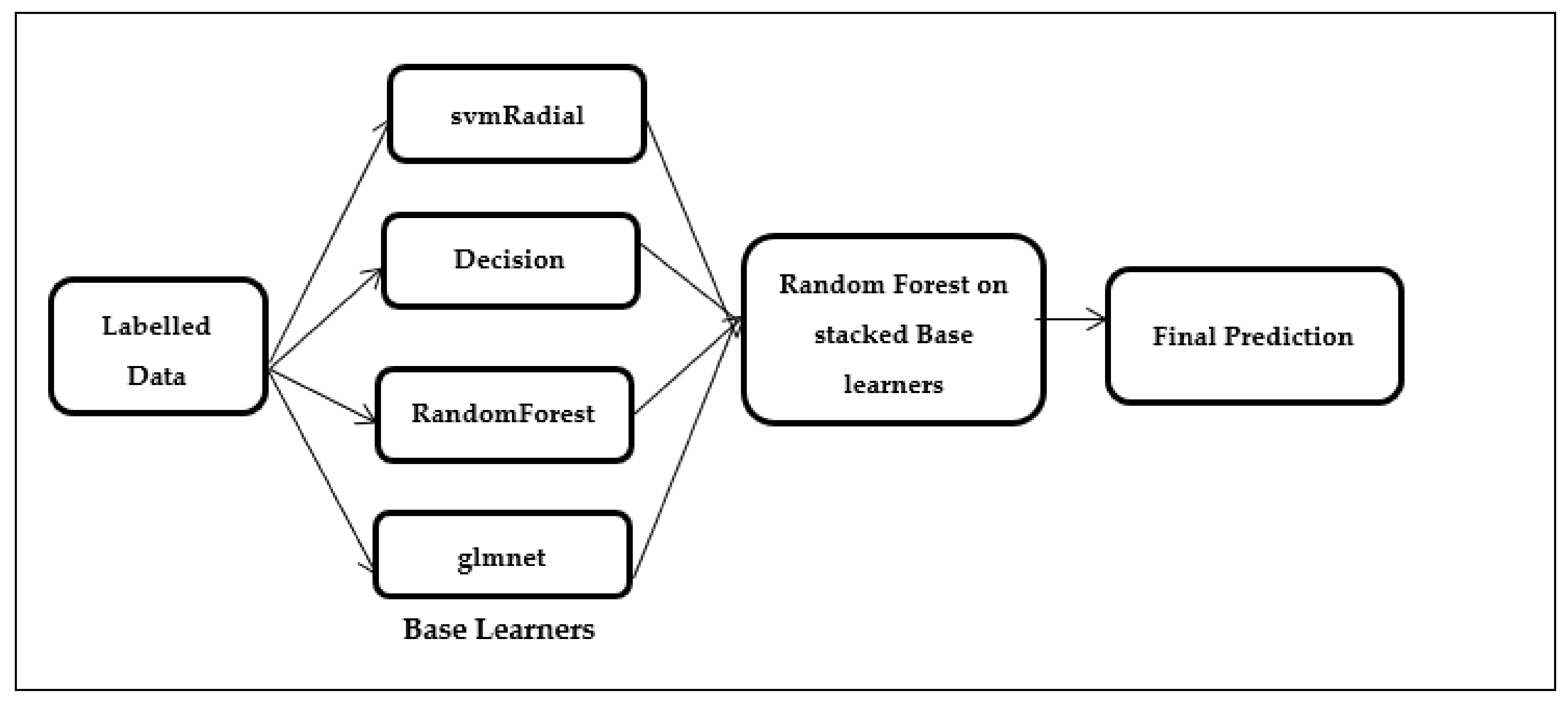
3.2. Proposed Stacking Using Random Forest for Estimation
| Algorithm 1. Pseudocode of proposed stacking using random forest. |
| 1. Input: Training data, Dtrain = where = Input attributes, = Output attribute, i = 1 to n, n = Number of base classifiers. |
| 2. Output: Ensemble classifier, E |
| 3. Step 1: Learn about base-level classifiers |
| (Apply first-level classifier) |
| Base-level classifiers considered were svmRadial, decision tree (rpart), RandomForest(rf), and glmnet |
| 4. for t = 1 to T do |
| 5. learn based on Dtrain |
| 6. end for |
| 7. Step 2: Build a new dataset for predictions based on the output of the base classifier with the new dataset |
| 8. for i = 1 to n do |
| 9. |
| where |
| 10. end for |
| 11. Step 3: Learn a meta classifier. Apply second-level classifier for the new dataset |
| Random Forest(rf) applied over the stacked base classifiers svm Radial, rpart, rf and glmnet (Figure 2) |
| 12. Learn E based on |
| 13. Return E (ensemble classifier) |
| 14. Predicted software effort estimation evaluation metrics using the ensemble approach are as follows: |
| 15. Mean absolute error (MAE) = |
| where ‘n’ is the total number of data points, is the original value and is the predicted value. |
| 16. Root mean squared error (RMSE) = |
| where ‘n’ is the total number of data points, is the original value, and is the predicted value. |
| 17. R-squared=, where RSS is the residual sum of squares and TSS is the total sum of squares. |
4. Data Preparation
Software Effort Estimation Datasets
5. Results and Discussion
5.1. Stacking Models
5.2. Proposed Stacking Using Random Forest against Single Base Learners and Ensemble Techniques for Estimation
6. Conclusions
Author Contributions
Funding
Data Availability Statement
Conflicts of Interest
References
- Sehra, S.K.; Brar, Y.S.; Kaur, N.; Sehra, S.S. Research patterns and trends in software Effort Estimation. Inf. Softw. Technol. 2017, 91, 1–21. [Google Scholar] [CrossRef]
- Sharma, A.; Kushwaha, D.S. Estimation of Software Development Effort from Requirements Based Complexity. Procedia Technol. 2012, 4, 716–722. [Google Scholar] [CrossRef]
- Silhavy, R.; Silhavy, P.; Prokopova, Z. Using Actors and Use Cases for Software Size Estimation. Electronics 2021, 10, 592. [Google Scholar] [CrossRef]
- Denard, S.; Ertas, A.; Mengel, S.; Ekwaro-Osire, S. Development Cycle Modeling: Resource Estimation. Appl. Sci. 2020, 10, 5013. [Google Scholar] [CrossRef]
- Park, B.K.; Kim, R. Effort Estimation Approach through Extracting Use Cases via Informal Requirement Specifications. Appl. Sci. 2020, 10, 3044. [Google Scholar] [CrossRef]
- Priya Varshini, A.G.; Anitha Kumari, K. Predictive analytics approaches for software Effort Estimation: A review. Indian J. Sci. Technol. 2020, 13, 2094–2103. [Google Scholar] [CrossRef]
- Jorgensen, M. Practical Guidelines for Expert-Judgment-Based Software Effort Estimation. IEEE Softw. 2005, 22, 57–63. [Google Scholar] [CrossRef]
- Satapathy, S.M.; Rath, S.K.; Acharya, B.P. Early stage software Effort Estimation using random forest technique based on use case points. IET Softw. 2016, 10, 10–17. [Google Scholar] [CrossRef]
- Anandhi, V.; Chezian, R.M. Regression Techniques in Software Effort Estimation Using COCOMO Dataset. In Proceedings of the International Conference on Intelligent Computing Applications, Coimbatore, India, 6–7 March 2014; pp. 353–357. [Google Scholar]
- García-Floriano, A.; López-Martín, C.; Yáñez-Márquez, C.; Abran, A. Support vector regression for predicting software enhancement effort. Inf. Softw. Technol. 2018, 97, 99–109. [Google Scholar] [CrossRef]
- Nassif, A.B.; Ho, D.; Capretz, L.F. Towards an early software estimation using log-linear regression and a multilayer perceptron model. J. Syst. Softw. 2013, 86, 144–160. [Google Scholar] [CrossRef]
- Baskeles, B.; Turhan, B.; Bener, A. Software Effort Estimation using machine learning methods. In Proceedings of the 22nd International Symposium on Computer and Information Sciences, Ankara, Turkey, 7–9 November 2007. [Google Scholar]
- Nassif, A.B.; Azzeh, M.; Idri, A.; Abran, A. Software Development Effort Estimation Using Regression Fuzzy Models. Comput. Intell. Neurosci. 2019, 2019. [Google Scholar] [CrossRef]
- Idri, A.; Hosni, M.; Abran, A. Improved Estimation of Software Development Effort Using Classical and Fuzzy Analogy Ensembles. Appl. Soft Comput. J. 2016, 49, 990–1019. [Google Scholar] [CrossRef]
- Hidmi, O.; Sakar, B.E. Software Development Effort Estimation Using Ensemble Machine Learning. Int. J. Comput. Commun. Instrum. Eng. 2017, 4, 1–5. [Google Scholar]
- Minku, L.L.; Yao, X. Ensembles and locality: Insight on improving software Effort Estimation. Inf. Softw. Technol. 2013, 55, 1512–1528. [Google Scholar] [CrossRef]
- Varshini, A.G.P.; Kumari, K.A.; Janani, D.; Soundariya, S. Comparative analysis of Machine learning and Deep learning algorithms for Software Effort Estimation. J. Phys. Conf. Ser. 2021, 1767, 12019. [Google Scholar] [CrossRef]
- Idri, A.; Amazal, F.a.; Abran, A. Analogy-based software development Effort Estimation: A systematic mapping and review. Inf. Softw. Technol. 2015, 58, 206–230. [Google Scholar] [CrossRef]
- Kumar, P.S.; Behera, H.S.; Kumari, A.; Nayak, J.; Naik, B. Advancement from neural networks to deep learning in software Effort Estimation: Perspective of two decades. Comput. Sci. Rev. 2020, 38, 100288. [Google Scholar] [CrossRef]
- Fedotova, O.; Teixeira, L.; Alvelos, H. Software Effort Estimation with Multiple Linear Regression: Review and Practical Application. J. Inf. Sci. Eng. 2013, 29, 925–945. [Google Scholar]
- Abdelali, Z.; Mustapha, H.; Abdelwahed, N. Investigating the use of random forest in software Effort Estimation. Procedia Comput. Sci. 2019, 148, 343–352. [Google Scholar] [CrossRef]
- Nassif, A.B.; Azzeh, M.; Capretz, L.F.; Ho, D. A comparison between decision trees and decision tree forest models for software development Effort Estimation. In Proceedings of the Third International Conference on Communications and Information Technology, Beirut, Lebanon, 19–21 June 2013. [Google Scholar]
- Corazza, A.; Di Martino, S.; Ferrucci, F.; Gravino, C.; Mendes, E. Using Support Vector Regression for Web Development Effort Estimation. In International Workshop on Software Measurement; Abran, A., Braungarten, R., Dumke, R.R., Cuadrado-Gallego, J.J., Brunekreef, J., Eds.; Springer: Heidelberg, Germany, 2009; Volume 5891, pp. 255–271. [Google Scholar]
- Marapelli, B. Software Development Effort Duration and Cost Estimation using Linear Regression and K-Nearest Neighbors Machine Learning Algorithms. Int. J. Innov. Technol. Explor. Eng. 2019, 9, 2278–3075. [Google Scholar]
- Hudaib, A.; Zaghoul, F.A.L.; Widian, J.A.L. Investigation of Software Defects Prediction Based on Classifiers (NB, SVM, KNN and Decision Tree). J. Am. Sci. 2013, 9, 381–386. [Google Scholar]
- Wu, J.H.C.; Keung, J.W. Utilizing cluster quality in hierarchical clustering for analogy-based software Effort Estimation. In Proceedings of the 8th IEEE International Conference on Software Engineering and Service Science, Beijing, China, 20–22 November 2017; pp. 1–4. [Google Scholar]
- Sree, P.R.; Ramesh, S.N.S.V.S.C. Improving Efficiency of Fuzzy Models for Effort Estimation by Cascading & Clustering Techniques. Procedia Comput. Sci. 2016, 85, 278–285. [Google Scholar]
- Rijwani, P.; Jain, S. Enhanced Software Effort Estimation Using Multi Layered Feed Forward Artificial Neural Network Technique. Procedia Comput. Sci. 2016, 89, 307–312. [Google Scholar] [CrossRef]
- Nassif, A.B.; Azzeh, M.; Capretz, L.F.; Ho, D. Neural network models for software development Effort Estimation: A comparative study. Neural Comput. Appl. 2015, 2369–2381. [Google Scholar] [CrossRef]
- Pospieszny, P.; Czarnacka-Chrobot, B.; Kobylinski, A. An effective approach for software project effort and duration estimation with machine learning algorithms. J. Syst. Softw. 2018, 137, 184–196. [Google Scholar] [CrossRef]
- Mensah, S.; Keung, J.; Bosu, M.F.; Bennin, K.E. Duplex output software Effort Estimation model with self-guided interpretation. Inf. Softw. Technol. 2018, 94, 1–13. [Google Scholar] [CrossRef]
- Singala, P.; Kumari, A.C.; Sharma, P. Estimation of Software Development Effort: A Differential Evolution Approach. In Proceedings of the International Conference on Computational Intelligence and Data Science, Gurgaon, India, 6–7 September 2019. [Google Scholar]


| Existing Work | Datasets | Algorithm | Evaluation Measures | Findings |
|---|---|---|---|---|
| Idri et al. [18] | Desharnais, ISBSG (International Software Benchmarking Standards Group), Albrecht, COCOMO, Kemerer, Maxwell, Abran, and Telecom | Analogy-based software effort estimation (ASEE) | (MMRE)-Mean Magnitude of Relative Error (MdMRE)-Median Magnitude of Relative Error (Pred(25)-Prediction percentage with an MRE less than or equal to 25% | The authors compared analogy-based software effort estimation (ASEE) with eight ML and Non-ML techniques such as the COCOMO model, regression, expert judgment, artificial neural network, function point analysis, support vector regression, decision trees, and radial basis function. From the results, the ASEE technique outperformed eight techniques and provided more accuracy based on the three evaluation measures, namely MMRE, MdMRE, and Pred(25). Several techniques such as fuzzy logic, genetic algorithm, expert judgment, artificial neural network, etc., are combined with ASEE methods. Fuzzy logic and genetic algorithm combined with ASEE provided good results compared with other combined techniques. It was found that estimation accuracy increased when ML and Non-ML techniques were combined with the ASEE technique. |
| Suresh Kumar et al. [19] | Commonly used datasets: COCOMO, NASA, and ISBSG | Analysis of SEE using artificial neural network algorithms (ANN) | Commonly used metrics:(MMRE)-Mean Magnitude of Relative Error, (MRE)-Mean Relative Error | In this paper, analysis of software effort estimation using various ANN algorithms such as a higher-order neural network, basic NN and a deep learning network was carried out. This paper mainly focused on comparing the quantitative and qualitative analysis of the papers under software effort estimation. They also created a survey on the following aspects: the most frequently used datasets for prediction, most frequent hybrid algorithm considered for prediction, and most-used evaluation measures, namely MMRE, MdMRE, and MRE. |
| Fedotova et al. [20] | Real time data of a mid-level multinational software development company | Multiple linear regression (MLR) | (MRE)-Mean Relative Error (MMRE)-Mean Magnitude of Relative Error, Pred(x)-Prediction percentage with an MRE less than or equal to x% | The project was carried out using a real-time dataset of a medium-sized multinational organization. This paper compared multiple linear regression (MLR) with the expert judgment method; MLR produced good results compared with expert judgment. Evaluation metrics considered were MRE, MMRE, and Pred(x). |
| Abdelali et al. [21] | ISBSG R8, Tukutuku, and COCOMO. | random forest | Pred(0.25), MMRE, and MdMRE | In this paper, the random forest algorithm was compared with the regression tree model. Before using the random forest algorithm, they explored the impact of the number of trees and the number of attributes to accuracy and found accuracy was sensitive to these parameters. Finally, the optimized random forest outperformed the regression tree algorithm. |
| Nassif et al. [22] | ISBSG 10 Desharnais | Decision tree, decision tree forest, andmultiple linear regression | Pred(0.25), MMRE and MdMRE | The decision tree forest model was compared with the traditional decision tree model and multiple linear regression. The evaluation was performed using ISBSG and Desharnais datasets. Decision tree uses a recursive partitioning approach, whereas the decision tree forest model is a collection of decision trees that are grown in parallel. The decision tree forest model outperformed the decision tree model and multiple linear regressionwhen the evaluation measures used were MMRE, MdMRE, and PRED (0.25). |
| Corazza et al. [23] | TUKUTUKU Dataset | Support Vector Regression | (Pred(25)) (MEMRE)-Mean Magnitude of Relative Error relative to the estimate (MdEMRE)-Median Magnitude of Relative Error relative to the estimate. | The authors compared Support Vector Regression (SVR) with step-wise, case-based reasoning and Bayesian network; SVR outperformed the other compared algorithms. Four kernel methods of SVR were considered for estimation, namely linear, Gaussian, polynomial, and sigmoid. Two preprocessing methods, namely logarithmic and normalization approaches, were carried out over the dataset. Final results showed that SVR with linear kernel and logarithmic transformation provides better results. |
| Bhaskar [24] | COCOMO81, COCOMO Nasa, and COCOMO Nasa2 | Linear regression and K nearest neighbor | Mean squared error (MSE) and Mean magnitude relative error (MMRE) | In this paper, the authors proposed that linear regression and K nearest neighbor (KNN) algorithms forecasted the effort accurately. The advantage of linear regression is it is fast at training the data and it produces good results when the output attribute is linear to the input attribute. KNN algorithms are preferred when there is less past knowledge regarding the data description. |
| Amjad et al. [25] | NASA Dataset | Naïve Bayes, support vector machine, K nearest neighbor, decision trees | F1, Precision and Recall | Software defect prediction was carried out using Naïve Bayes, support vector machine, K nearest neighbor (KNN), and decision trees. KNN is a simple model, and uses a statistical approach; Naïve Bayes is a probabilistic model that uses the Bayes theorem; and decision trees uses the recursive partitioning approach and SVM used for both structured and unstructured data. In this paper, the NASA dataset was used and the Naïve Bayes algorithm outperformed the support vector, KNN, and decision tree. |
| Wu et al. [26] | Desharnais, Cocomo81, Maxwell, China, Nasa93, and Kemerer | Hierarchical clustering for analogy-based software effort estimation (ABE) | MMRE-Mean Magnitude Relative Error | The research was carried out using analogy-based software effort estimation (ABE), which uses case-based reasoning that depends on the K value (K-th similar project that is completed over the past). The hierarchical clustering technique was used to identify the optimized set of K values. The proposed hierarchical clustering to the ABE method showed good improvement to ABE. |
| Sree et al. [27] | NASA 93 | Fuzzy model using subtractive clustering | Variance Accounted For(VAF) Mean Absolute Relative Error(MARE) Variance Absolute relative Error(VARE) Mean Balance Relative Error(Mean BRE) Mean Magnitude of Relative Error(MMRE) Prediction | In this paper, the fuzzy model using subtractive clustering used three rules and provided better estimates compared with cascading the fuzzy logic controller. The computational time for fuzzy logic controller was higher because the rule base was quite large. To reduce the rule base, cascading fuzzy logic controllers were used and to find the correct number of cascading, a subtractive clustering method was employed. |
| Rijwani et al. [28] | COCOMO II | Multi-layered feed forward artificial neural network | Mean-Square-Error (MSE) and Mean Magnitude of Relative Error (MMRE) | Artificial Neural Network (ANN) can handle complex datasets with various dependent and independent variables. Multi-layered Feed Forward ANN with backpropagation method is employed over here. Multi-layered Feed Forward ANN provided better results and accuracy in forecasting effort. |
| Nassif et al. [29] | International Software Benchmarking Standards Group (ISBSG) | Multilayer perceptron; general regression neural network; radial basis function neural network; cascade correlation neural network | Mean Absolute Residual (MAR) | Models considered for estimation are General Regression Neural Network, Multilayer Perceptron, Radial Basis Function Neural Network and Cascade Correlation Neural Network. In comparison with the four models, 3 models overestimate the accuracy and Cascade Correlation Neural Network outperforms other compared algorithms. ISBSG dataset is used for estimation. |
| Pospieszny et al. [30] | ISBSG 1192 projects 13 attributes | ensemble averaging of 3 ML models -SVM(support vector machines) MLP(multi- layer perceptron) -GLM(general linear model) | MAE, MSE, and RMSE MMRE PRED MMER- Mean magnitude relative error to estimate MBRE-mean of balanced relative error | The dataset used for estimation was the ISBSG dataset. Ensemble averaging of three machine learning algorithms was used for estimation. Three models considered for ensemble averaging were SVM (support vector machines), MLP (multi-layer perceptron), and GLM (general linear model). In ensemble, multiple base learners’ models were combined for effort estimation. The ensemble model outperformed the single models. |
| Mensah et al. [31] | Github: Albrecht Telecom PROMISE: China Cocomo Cocomonasa1 Cocomonasa Cosmic Desharnais Kemerer Kitchenham Maxwell Miyazaki Industry:php_projects | Regression-based effort estimation techniques: ordinary least squares regression (OLS), stepwise regression (SWR), ridge regression (RR), LASSO regression, elastic net regression, | Mean Absolute Error(MAE), Balanced Mean Magnitude of Relative Error (BMMRE) and Adjusted R2 | Software Effort Estimation models incur a drawback in prediction termed conclusion instability. In this paper, 14 datasets are considered for estimation and based on the effort attribute each dataset are grouped into three classes namely high, low and medium which is considered as the first output and again to the effort classes, six regression models were applied to predict accuracy which is considered as the second output. Elastic net regression outperformed the other compared algorithms. |
| Prerna et al. [32] | cocomo81 and nasa93 | differential evolution (DE) approach | MMRE | The differential evolution (DE) approach was applied over COCOMO and COCOMO II models for the datasets from the PROMISE repository. DE approach produced less computational complexity and less memory utilization. The Proposed DE-based COCOMO and COCOMO II approach provided better effort estimates compared with the original COCOMO and COCOMO II models. |
| Dataset Name | Source Repository | No. of Records | No. of Attributes | Output Attribute-Effort (Unit) |
|---|---|---|---|---|
| (i) Albrecht | PROMISE | 24 | 8 | Person-months |
| (ii) China | PROMISE | 499 | 16 | Person-hours |
| (iii) Desharnais | GITHUB | 81 | 12 | Person-hours |
| (iv) Kemerer | GITHUB | 15 | 7 | Person-months |
| (v) Maxwell | PROMISE | 62 | 27 | Person-hours |
| (vi) Kitchenham | GITHUB | 145 | 9 | Person-hours |
| (vii) Cocomo81 | GITHUB | 63 | 17 | Person-months |
| Datasets Name | Attributes and Description | Attributes Considered after Feature Selection | |
|---|---|---|---|
| Albrecht | InputNumeric | Count of input functions |
|
| OutputNumeric | Count of output functions | ||
| InquiryNumeric | Count of query functions | ||
| FileNumeric | Count of file processing | ||
| FPAdjNumeric | Function point | ||
| RawFPcounsNumeric | Raw function points | ||
| AdjfpNumeric | Adjusted function points | ||
| Effort | Effort in person-months | ||
| China | AFP | Adjusted function points |
|
| Input | Function points of input | ||
| Output | Function points of external output | ||
| Enquiry | Function points of external output enquiry | ||
| File | Function points of internal logical files | ||
| Interface | Function points of external interface added | ||
| Added | Function points of added functions | ||
| Changed | Function points of changed functions | ||
| PDR_AFP | Productivity delivery rate(adjusted function points) | ||
| PDR_UFP | Productivity delivery rate(Unadjusted function points) | ||
| NPDR_AFP | Normalized productivity delivery rate(adjusted function points) | ||
| NPDU_UFP | Productivity delivery rate(Unadjusted function points) | ||
| Resource | Team type | ||
| Duration | Total elapsed time for the project | ||
| N-Effort | Normalized effort | ||
| Effort | Summary work report | ||
| Desharnais | Project | Project number |
|
| TeamExp | Team experience in years | ||
| ManagerExp | Project manager’s experience in years | ||
| YearEnd | Year of completion | ||
| Length | Length of the project | ||
| Transactions | Number of transactions processed | ||
| Entities | Number of entities | ||
| PointsNonAdjust | Unadjusted function points | ||
| Adjustment | Adjustment factor | ||
| PointsAjust | Adjusted function points | ||
| Language | Programming language | ||
| Effort | Measured in person-hours | ||
| Kemerer | Language | Programming language |
|
| Hardware | Hardware resources | ||
| Duration | Duration of the project | ||
| KSLOC | Kilo lines of code | ||
| AdjFP | Adjusted function points | ||
| RawFP | Unadjusted function points | ||
| Effort | Measured in person-months | ||
| Maxwell | Year | Time |
|
| App | Application type | ||
| Har | Hardware platform | ||
| Dba | Database | ||
| Ifc | User interface | ||
| Source | Where developed | ||
| Telonuse | Telon use | ||
| Nlan | Number of development languages | ||
| T01 | Customer participation | ||
| T02 | Development environment adequacy | ||
| T03 | Staff availability | ||
| T04 | Standards use | ||
| T05 | Methods use | ||
| T06 | Tools use | ||
| T07 | Software logical complexity | ||
| T08 | Requirements volatility | ||
| T09 | Quality requirements | ||
| T10 | Efficiency requirements | ||
| T11 | Installation requirements | ||
| T12 | Staff analysis skills | ||
| T13 | Staff application knowledge | ||
| T14 | Staff tool skills | ||
| T15 | Staff team skills | ||
| Duration | Duration (months) | ||
| Size | Application size (FP) | ||
| Time | Time taken | ||
| Effort | Work carried out in person-hours | ||
| Kitchenham | Clientcode | Client code {1,2,3,4,5,6} |
|
| Projecttype | Project Type {A,C,D,P,Pr,U} | ||
| Startdate | Starting date of the project | ||
| Duration | Duration of the project | ||
| Adjfp | Adjusted function points | ||
| Completiondate | Completion date of the project | ||
| Estimate | Effort estimate | ||
| Estimate method | Estimate method {A,C,CAE,D,EO,W} | ||
| Effort | Work carried out in person-hours | ||
| Cocomo81 | Rely | Required software reliability |
|
| Data | Database size | ||
| Cplx | Complexity of product | ||
| Time | Time constraint | ||
| Stor | Storage constraint | ||
| Virt | Virtual machine volatility | ||
| Turn | Computer turnaround time | ||
| Acap | Analyst capability | ||
| Aexp | Application experience | ||
| Pcap | Programmer capability | ||
| Vexp | Virtual machine experience | ||
| Lexp | Programming language experience | ||
| Modp | Modern programming practices | ||
| Tool | Software tools use | ||
| Sced | Development schedule | ||
| Loc | Lines of code | ||
| Effort | Work carried in person-months | ||
| Mean Absolute Error (MAE) | |||||||
|---|---|---|---|---|---|---|---|
| Algorithms | Dataset 1 Albrecht | Dataset 2 China | Dataset 3 Desharnais | Dataset 4 Kemerer | Dataset 5 Maxwell | Dataset 6 Kitchenham | Dataset 7 Cocomo81 |
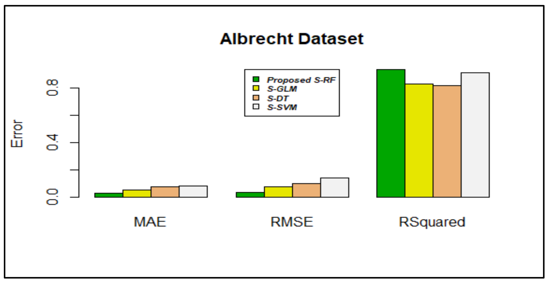
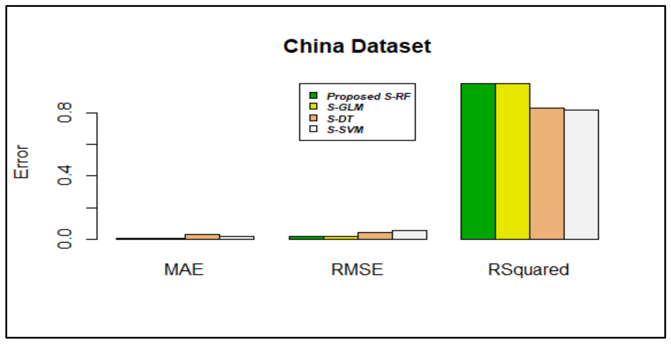
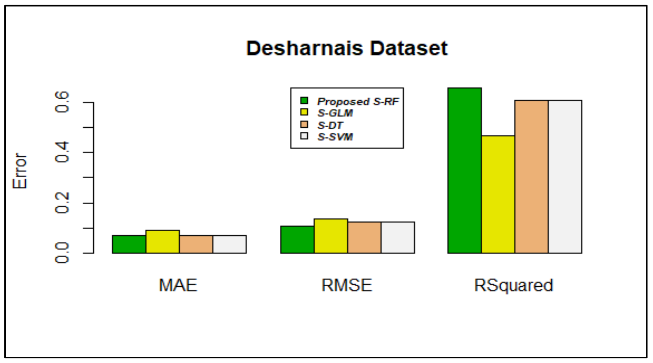
| Random Forest | 0.1940703 | 0.03832486 | 0.1161946 | 0.2076936 | 0.2330224 | 0.1047124 | 0.06047924 |
| SVM | 0.271210 | 0.04872961 | 0.1052762 | 0.219517 | 0.311288 | 0.1189372 | 0.07500071 |
| Decision Tree | 0.2299442 | 0.0222997 | 0.1067227 | 0.3709271 | 0.2896955 | 0.1174008 | 0.08838886 |
| Neuralnet | 0.2208348 | 0.01775594 | 0.08394905 | 0.2179616 | 0.2245069 | 0.03921013 | 0.05387155 |
| Ridge | 0.2495593 | 0.01977087 | 0.08810373 | 0.1971335 | 0.2162983 | 0.04342892 | 0.07912894 |
| LASSO | 0.2672776 | 0.01344521 | 0.08731722 | 0.183967 | 0.2106617 | 0.03876806 | 0.08097285 |
| ElasticNet | 0.2522743 | 0.01406866 | 0.08874032 | 0.1890074 | 0.211274 | 0.03961122 | 0.07980254 |
| Deepnet | 0.2702398 | 0.09730134 | 0.1913845 | 0.4011895 | 0.2901784 | 0.1400501 | 0.2548906 |
| Averaging | 0.2133583 | 0.01996002 | 0.09603559 | 0.239746 | 0.09006789 | 0.01797183 | 0.06160017 |
| Weighted Averaging | 0.1658832 | 0.05308728 | 0.1378911 | 0.1811016 | 0.1211871 | 0.02715146 | 0.06493144 |
| Bagging | 0.1784421 | 0.01207605 | 0.1195285 | 0.2042914 | 0.2356023 | 0.009002502 | 0.08604002 |
| Boosting | 0.1237017 | 0.01059957 | 0.1072595 | 0.2345743 | 0.08203951 | 0.009002502 | 0.08095949 |
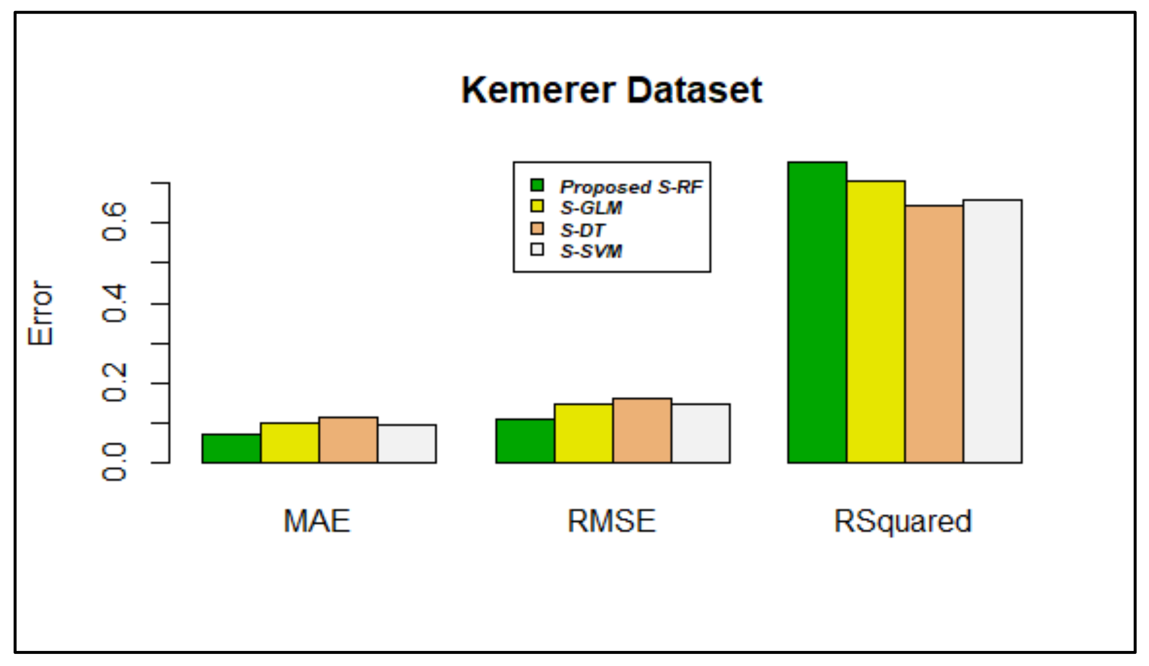
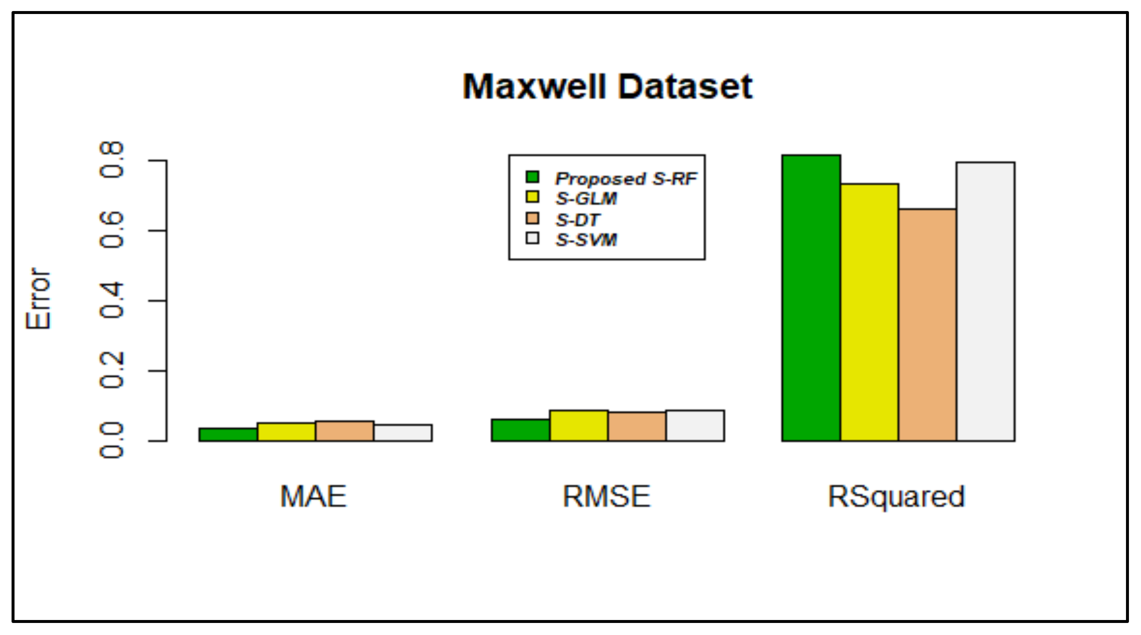
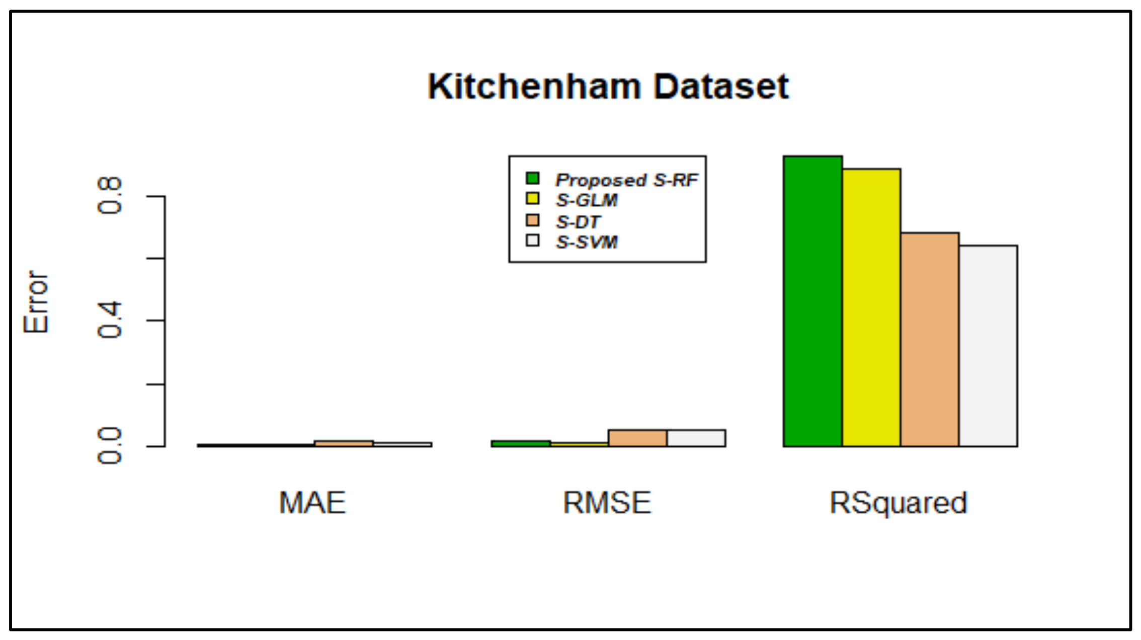
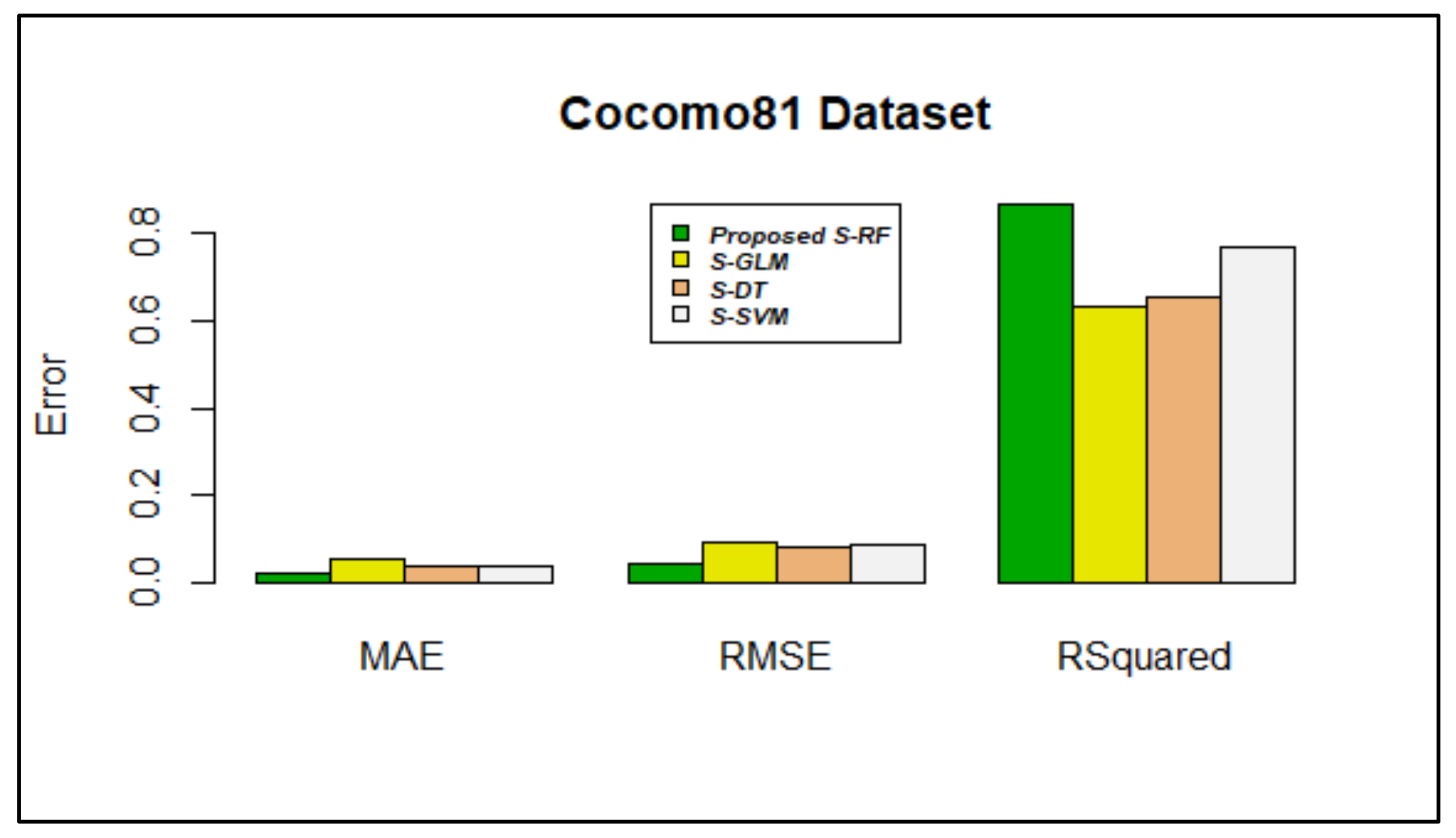
| Proposed Stacking using RF | 0.0288617 | 0.004016189 | 0.07027704 | 0.07030604 | 0.03566583 | 0.005384577 | 0.02278088 |
| Root Mean Squared Error (RMSE) | |||||||
|---|---|---|---|---|---|---|---|
| Algorithms | Dataset 1 Albrecht | Dataset 2 China | Dataset 3 Desharnais | Dataset 4 Kemerer | Dataset 5 Maxwell | Dataset 6 Kitchenham | Dataset 7 Cocomo81 |
| Random Forest | 0.2273109 | 0.0651549 | 0.1744573 | 0.2357751 | 0.3098055 | 0.1715596 | 0.1402015 |
| SVM | 0.291869 | 0.109964 | 0.1993475 | 0.2635159 | 0.4006657 | 0.2379881 | 0.1976564 |
| Decision Tree | 0.3140069 | 0.05380968 | 0.1724028 | 0.3954624 | 0.3897197 | 0.2013018 | 0.1869692 |
| Neuralnet | 0.2676081 | 0.0439852 | 0.1508566 | 0.3219353 | 0.2914014 | 0.0739 | 0.09447618 |
| Ridge | 0.274339 | 0.03703651 | 0.1482106 | 0.2810334 | 0.2901234 | 0.08774596 | 0.1592412 |
| LASSO | 0.2952834 | 0.02381411 | 0.1455049 | 0.256731 | 0.2859893 | 0.07402251 | 0.1766792 |
| ElasticNet | 0.2771694 | 0.02462756 | 0.1463786 | 0.26093 | 0.2865395 | 0.07542022 | 0.1747383 |
| Deepnet | 0.3222748 | 0.1497018 | 0.2396687 | 0.4142278 | 0.3571974 | 0.2242306 | 0.285657 |
| Averaging | 0.2403676 | 0.06114447 | 0.1569477 | 0.2719905 | 0.1386882 | 0.04447122 | 0.1272475 |
| Weighted Averaging | 0.2789538 | 0.1214186 | 0.2275768 | 0.3253842 | 0.2096006 | 0.1059557 | 0.1831177 |
| Bagging | 0.2264107 | 0.04121619 | 0.1764452 | 0.2399795 | 0.3120326 | 0.02091779 | 0.176543 |
| Boosting | 0.184356 | 0.03618514 | 0.162724 | 0.2626449 | 0.1215997 | 0.02091779 | 0.1693169 |
| Proposed Stacking using RF | 0.0370489 | 0.01562433 | 0.1072363 | 0.1094053 | 0.06379541 | 0.01505940 | 0.04415005 |
| R-Squared | |||||||
|---|---|---|---|---|---|---|---|
| Algorithms | Dataset 1 Albrecht | Dataset 2 China | Dataset 3 Desharnais | Dataset 4 Kemerer | Dataset 5 Maxwell | Dataset 6 Kitchenham | Dataset 7 Cocomo81 |
| Random Forest | 0.4732279 | 0.8028527 | 0.38059 | 0.6032962 | 0.109088 | 0.3928102 | 0.6062928 |
| SVM | 0.1315232 | 0.4384377 | 0.1912367 | 0.5044536 | -0.4901189 | -0.1684357 | 0.2174898 |
| Decision Tree | 0.0052189 | 0.8655325 | 0.3950932 | -0.1160428 | -0.4098123 | 0.1640318 | 0.2998227 |
| Neuralnet | 0.2699029 | 0.9101517 | 0.5368423 | 0.2603814 | 0.2117937 | 0.8873365 | 0.8212226 |
| Ridge | 0.232714 | 0.9362975 | 0.5529472 | 0.4363801 | 0.2186921 | 0.8411641 | 0.4920992 |
| LASSO | 0.1110852 | 0.9736631 | 0.5691211 | 0.5296434 | 0.2407999 | 0.8869626 | 0.3747712 |
| ElasticNet | 0.2168 | 0.9718331 | 0.563931 | 0.5141316 | 0.2378761 | 0.8826536 | 0.3884329 |
| Deepnet | -0.05885081 | -0.0407606 | -0.169022 | -0.2244724 | -0.1843314 | -0.037252 | -0.6343981 |
| Averaging | 0.4109746 | 0.8263755 | 0.498686 | 0.4720681 | 0.5942589 | 0.9096699 | 0.6756852 |
| Weighted Averaging | 0.2066829 | 0.3153521 | -0.05403761 | 0.24444970 | 0.07326536 | 0.4872298 | 0.3283723 |
| Bagging | 0.4773922 | 0.9211081 | 0.3663932 | 0.5890217 | 0.09623293 | 0.9800149 | 0.3757349 |
| Boosting | 0.6855181 | 0.9478667 | 0.461106 | 0.5907376 | 0.6880857 | 0.9800149 | 0.425793 |
| Proposed Stacking using RF | 0.9357274 | 0.9839643 | 0.6556170 | 0.7520435 | 0.8120214 | 0.9246614 | 0.8667750 |
Publisher’s Note: MDPI stays neutral with regard to jurisdictional claims in published maps and institutional affiliations. |
© 2021 by the authors. Licensee MDPI, Basel, Switzerland. This article is an open access article distributed under the terms and conditions of the Creative Commons Attribution (CC BY) license (https://creativecommons.org/licenses/by/4.0/).
Share and Cite
A G, P.V.; K, A.K.; Varadarajan, V. Estimating Software Development Efforts Using a Random Forest-Based Stacked Ensemble Approach. Electronics 2021, 10, 1195. https://doi.org/10.3390/electronics10101195
A G PV, K AK, Varadarajan V. Estimating Software Development Efforts Using a Random Forest-Based Stacked Ensemble Approach. Electronics. 2021; 10(10):1195. https://doi.org/10.3390/electronics10101195
Chicago/Turabian StyleA G, Priya Varshini, Anitha Kumari K, and Vijayakumar Varadarajan. 2021. "Estimating Software Development Efforts Using a Random Forest-Based Stacked Ensemble Approach" Electronics 10, no. 10: 1195. https://doi.org/10.3390/electronics10101195
APA StyleA G, P. V., K, A. K., & Varadarajan, V. (2021). Estimating Software Development Efforts Using a Random Forest-Based Stacked Ensemble Approach. Electronics, 10(10), 1195. https://doi.org/10.3390/electronics10101195