A Cartesian Genetic Programming Based Parallel Neuroevolutionary Model for Cloud Server’s CPU Usage Prediction

 , , , and
Abstract
1. Introduction
- We present the mathematical model of CGP based neural network with parameters and hyperparameters;
- We evolve synaptic weights, topology, and the number of neurons for boosting learnability;
- We conduct multiple search path optimization to avoid local optima;
- We use a sliding window-based parallel architecture that makes several parallel predictions. These predictions are averaged for improving accuracy.
2. Purpose of Resource Prediction and Related Work
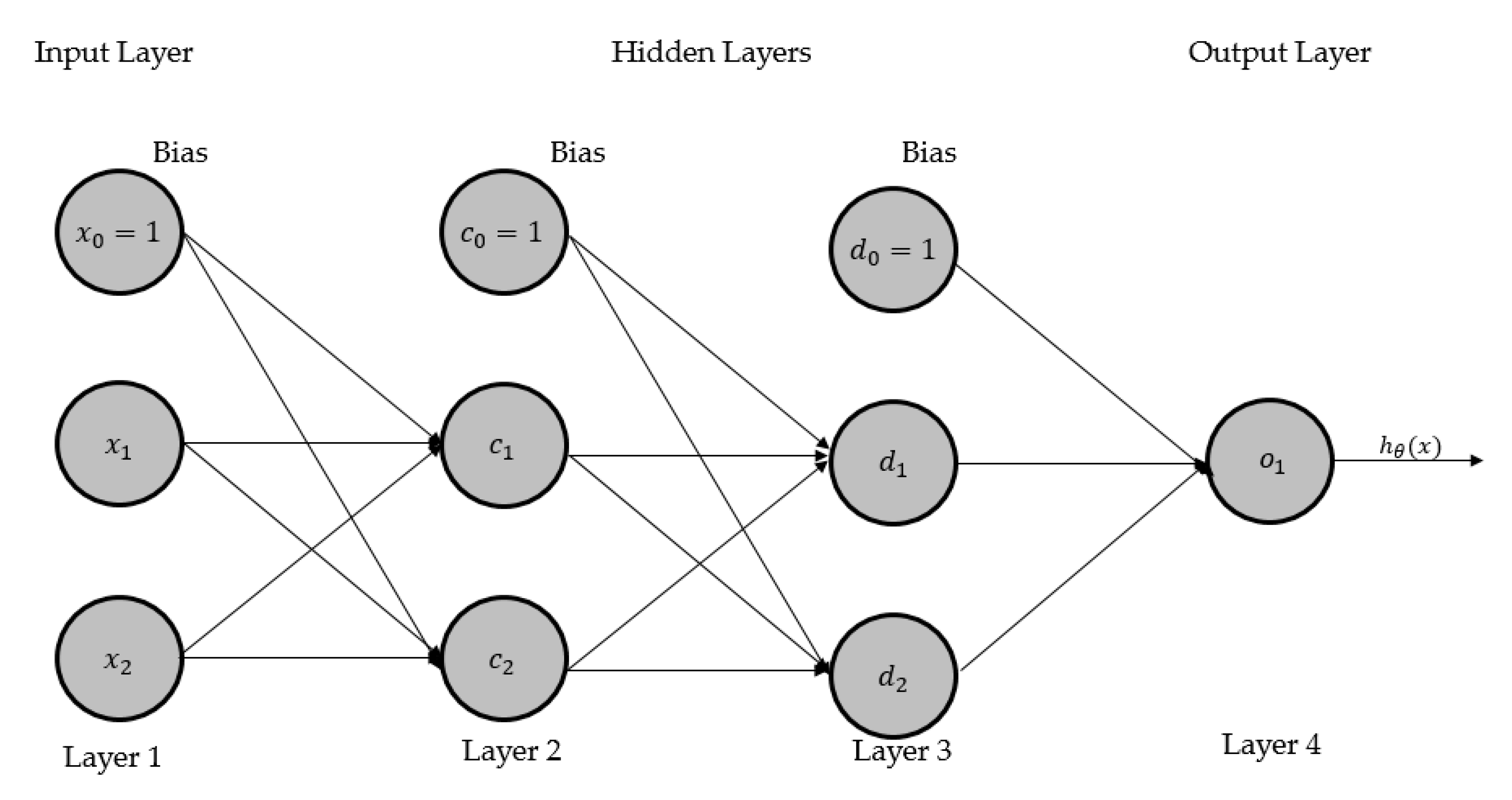
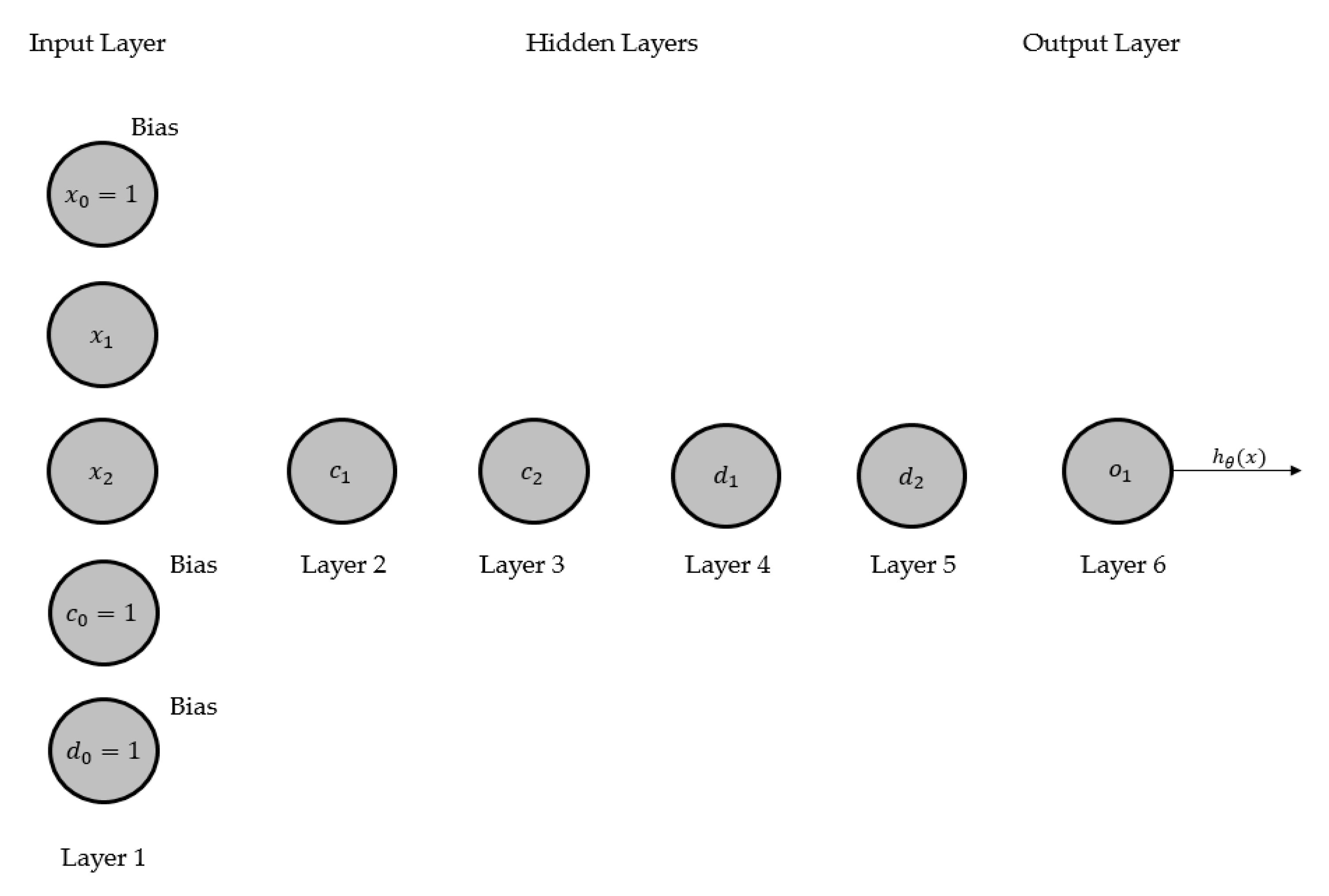
3. CGP-Based Neuroevolutionary Neural Network (CGPNN)
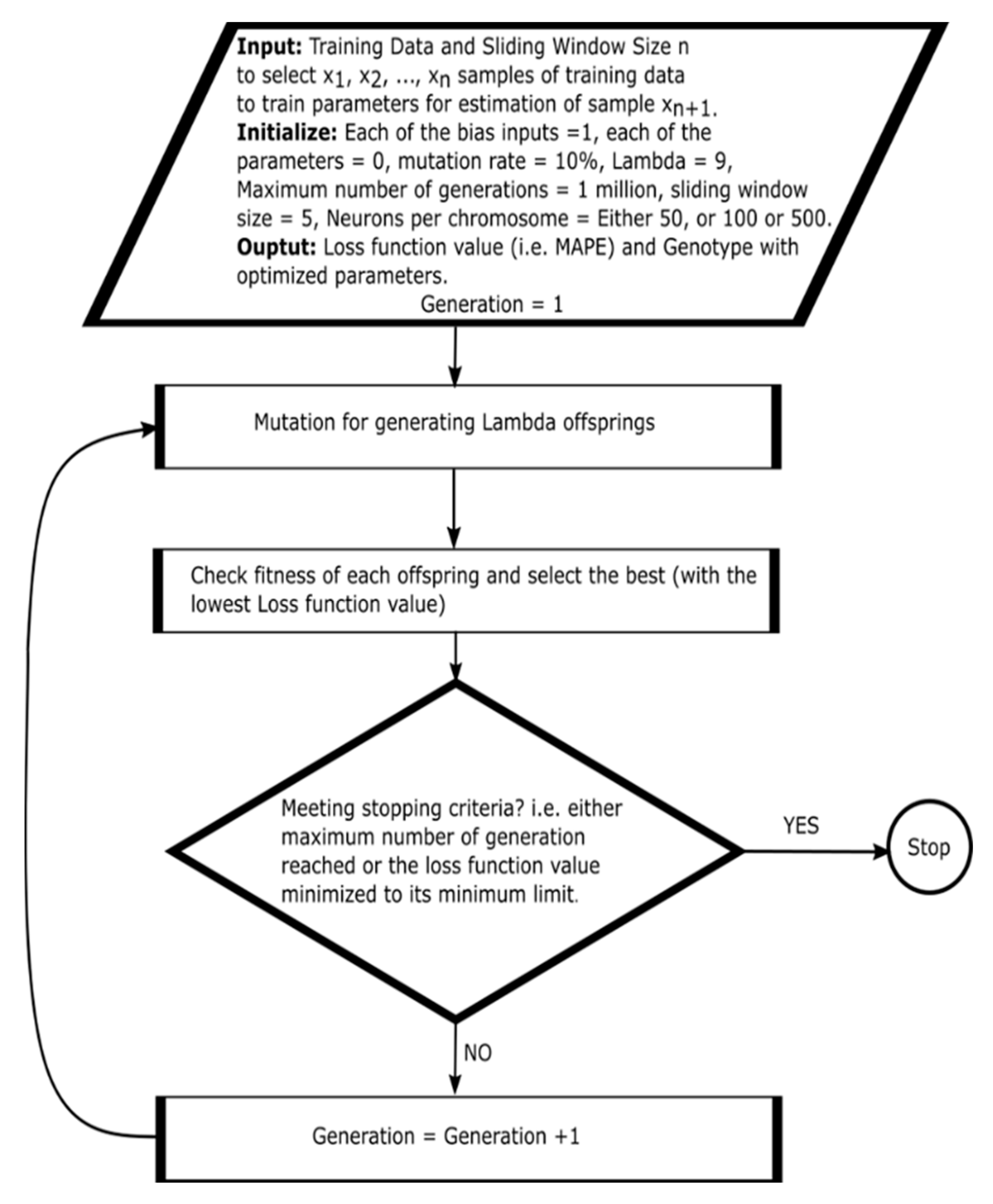
4. CGPNN Optimization Method
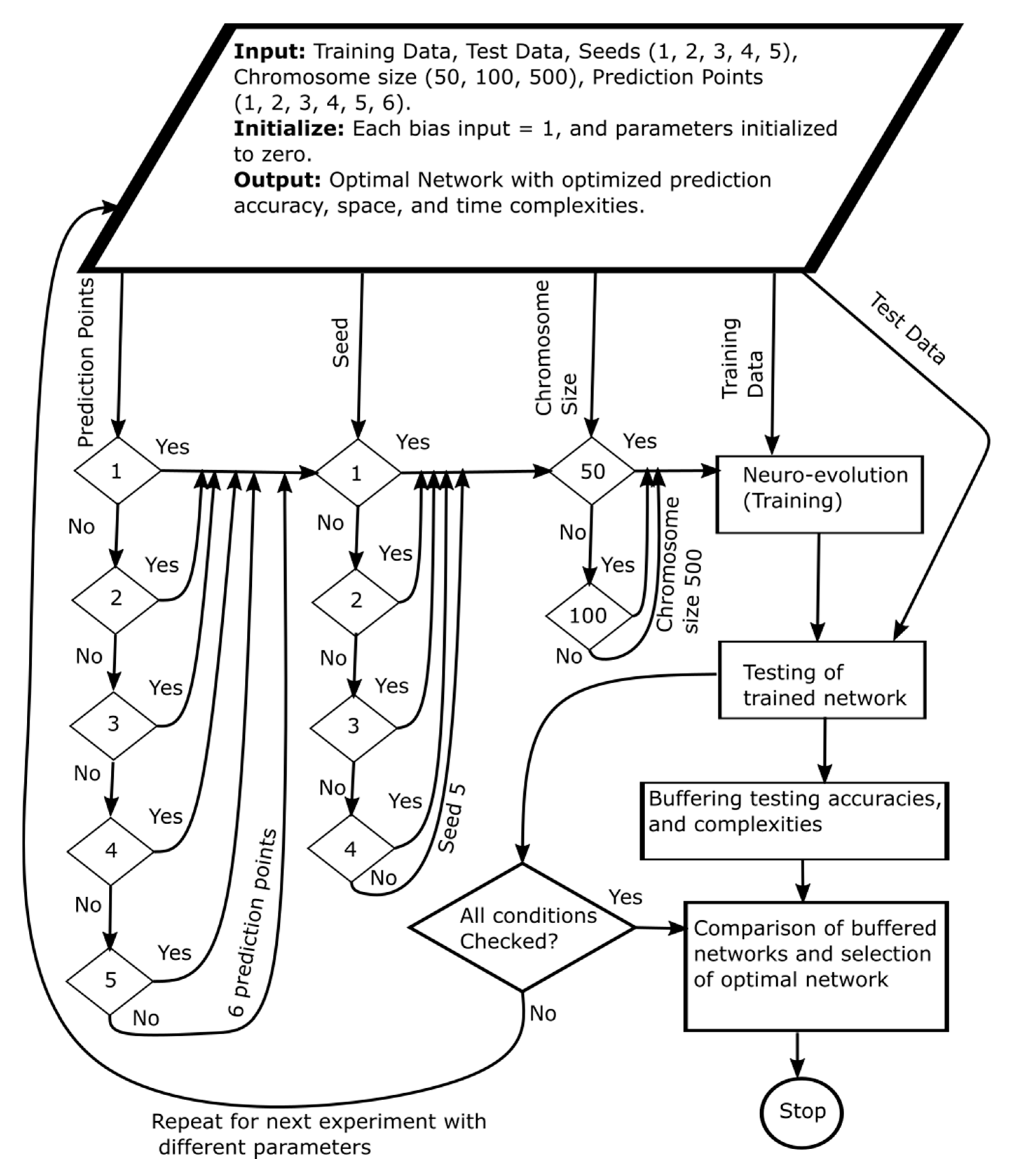
5. Experimental Platform and Methodology
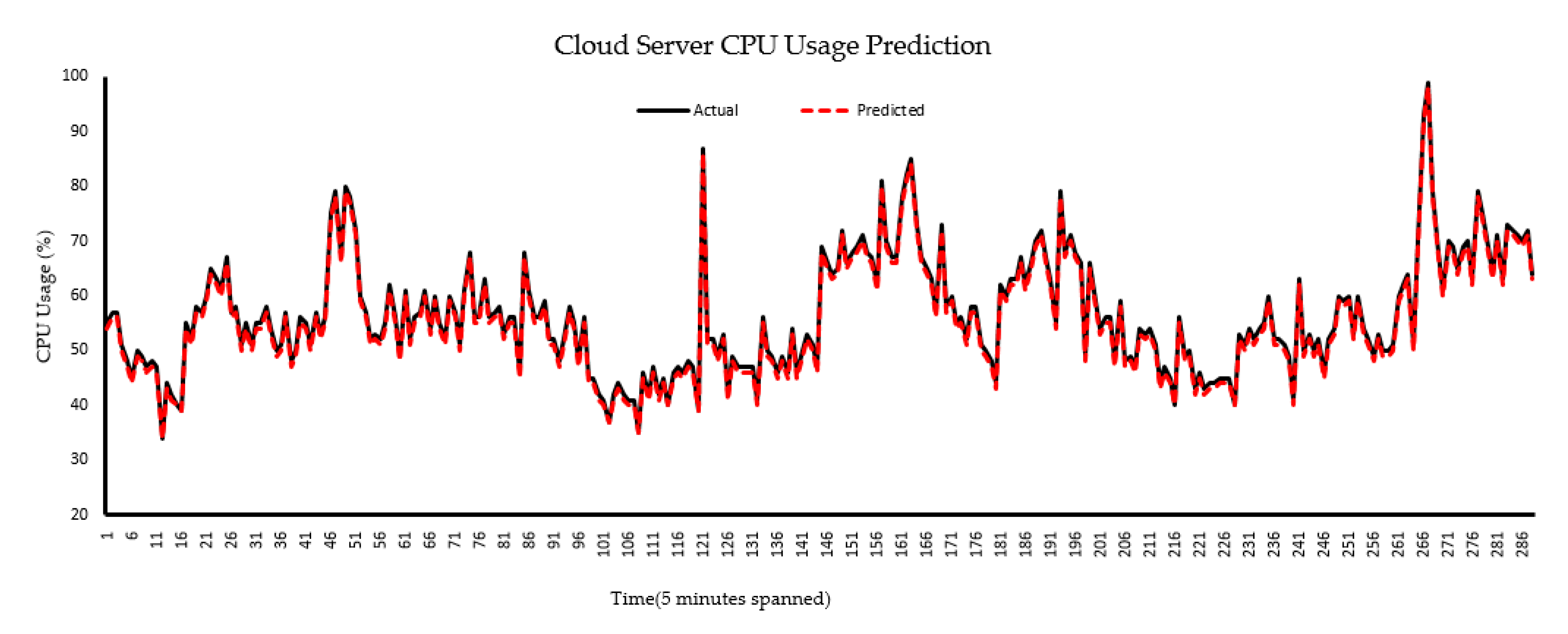
6. Results and Discussion
Comparison with Related Work
7. Conclusions and Future Directions
Author Contributions
Funding
Institutional Review Board Statement
Informed Consent Statement
Data Availability Statement
Conflicts of Interest
References
- Brown, R.; Masanet, E.R.; Nordman, B.; Tschudi, W.F.; Shehabi, A.; Stanley, J.; Koomey, J.G.; Sartor, D.A.; Chan, P.T. Report to Congress on Server and Data Center Energy Efficiency: Public Law 109–431; University of California: Berkeley, CA, USA, 2008. [Google Scholar]
- Uddin, M.; Rahman, A.A. Server consolidation: An approach to make data centers energy efficient and green. Int. J. Sci. Eng. Res. 2010, 1, 1. [Google Scholar] [CrossRef]
- Shang, L.; Peh, L.S.; Jha, N.K. Dynamic Voltage Scaling with Links for Power Optimization of Interconnection Networks. In Proceedings of the Ninth International Symposium on High-Performance Computer Architecture (HPCA’03), Anaheim, CA, USA, 8–12 February 2003; Volume 3, pp. 91–102. [Google Scholar]
- Dougherty, B.; White, J.; Schmidt, D.C. Model-driven auto-scaling of green cloud computing infrastructure. Future Gener. Comput. Syst. 2012, 28, 371–378. [Google Scholar] [CrossRef]
- Meisner, D.; Gold, B.T.; Wenisch, T.F. Powernap: Eliminating server idle power. ACM Sigplan Not. 2009, 44, 205–216. [Google Scholar] [CrossRef]
- Mwaikambo, Z.; Raj, A.; Russell, R.; Schopp, J.; Vaddagiri, S. Linux kernel hotplug cpu support. In Proceedings of the Linux Symposium, Ottawa, ON, Canada, 21–24 July 2004; Volume 2. [Google Scholar]
- Ullah, Q.Z.; Khan, G.M.; Hassan, S. Cloud Infrastructure Estimation and Auto-Scaling Using Recurrent Cartesian Genetic Programming-Based ANN. IEEE Access 2020, 8, 17965–17985. [Google Scholar] [CrossRef]
- Gandhi, A.; Chen, Y.; Gmach, D.; Arlitt, M.; Marwah, M. Minimizing data center SLA violations and power consumption via hybrid resource provisioning. In Proceedings of the 2011 International Green Computing Conference and Workshops, Orlando, FL, USA, 25–28 July 2011; pp. 1–8. [Google Scholar]
- Dabbagh, M.; Hamdaoui, B.; Guizani, M.; Rayes, A. Toward energy-efficient cloud computing: Prediction, consolidation, and overcommitment. IEEE Netw. 2015, 29, 56–61. [Google Scholar] [CrossRef]
- Moriarty, D.E.; Mikkulainen, R. Efficient reinforcement learning through symbiotic evolution. Mach. Learn. 1996, 22, 11–32. [Google Scholar] [CrossRef]
- Calheiros, R.N.; Masoumi, E.; Ranjan, R.; Buyya, R. Workload prediction using the Arima model and its impact on cloud application’s QoS. IEEE Trans. Cloud Comput. 2015, 3, 449–458. [Google Scholar] [CrossRef]
- Islam, S.; Keung, J.; Lee, K.; Liu, A. Empirical prediction models for adaptive resource provisioning in the cloud. Future Gener. Comput. Syst. 2012, 28, 155–162. [Google Scholar] [CrossRef]
- Zeileis, A. Dynlm: Dynamic Linear Regression; Cran: Innsbruck, Austria, 2019; Available online: https://cran.r-project.org/web/packages/dynlm/dynlm.pdf (accessed on 17 November 2020).
- Venables, W.N.; Ripley, B.D. Modern Applied Statistics with S-PLUS. In Statistics and Computing, 3rd ed.; Springer: New York, NY, USA, 2001. [Google Scholar]
- R Development Core Team. R: A Language and Environment for Statistical Computing; R Foundation for Statistical Computing: Vienna, Austria, 2010. [Google Scholar]
- Prevost, J.J.; Nagothu, K.; Kelley, B.; Jamshidi, M. Prediction of cloud data center networks loads using stochastic and neural models. In Proceedings of the 6th International Conference on System of Systems Engineering SoSE 2011, Albuquerque, NM, USA, 27–30 June 2011; pp. 276–281. [Google Scholar]
- Ismaeel, S.; Miri, A. Multivariate time series elm for cloud data center workload prediction. In Proceedings of the 18th International Conference on Human-Computer Interaction, Toronto, ON, Canada, 17–22 July 2016; pp. 565–576. [Google Scholar]
- Farahnakian, F.; Pahikkala, T.; Liljeberg, P.; Plosila, J. Energy-aware consolidation algorithm based on k-nearest neighbor regression for cloud data centers. In Proceedings of the 2013 IEEE/ACM 6th International Conference on Utility and Cloud Computing (UCC), Dresden, Germany, 9–12 December 2013; pp. 256–259. [Google Scholar]
- Nikravesh, A.; Yadavar, A.; Samuel, A.; Lung, C.-H. Towards an autonomic auto-scaling prediction system for cloud resource provisioning. In Proceedings of the 10th International Symposium on Software Engineering for Adaptive and Self-Managing Systems, Florence, Italy, 16–24 May 2015; pp. 35–45. [Google Scholar]
- Gong, Z.; Gu, X.; Wilkes, J. Press: Predictive elastic resource scaling for cloud systems. In Proceedings of the 6th International Conference on Network and Service Management (CNSM), Niagara Falls, ON, Canada, 25–29 October 2010; pp. 9–16. [Google Scholar]
- Sudevalayam, S.; Kulkarni, P. Affinity-aware modeling of CPU usage for provisioning virtualized applications. In Proceedings of the 2011 IEEE 4th International Conference on Cloud Computing, Washington, DC, USA, 4–9 July 2011; pp. 139–146. [Google Scholar]
- Ullah, Z.; Hassan, Q.S.; Khan, G.M. Adaptive Resource Utilization Prediction System for Infrastructure as a Service Cloud. Comput. Intell. Neurosci. 2017, 2017. [Google Scholar] [CrossRef]
- Duggan, M.; Mason, K.; Duggan, J.; Howley, E.; Barrett, E. Predicting host CPU utilization in cloud computing using recurrent neural networks. In Proceedings of the 2017 12th International Conference for Internet Technology and Secured Transactions (ICITST), Cambridge, UK, 11–14 December 2017. [Google Scholar]
- Rizvandi, N.B.; Taheri, J.; Moraveji, R.; Zomaya, A.Y. On modeling and prediction of total CPU usage for applications in MapReduce environments. In Proceedings of the International Conference on Algorithms and architectures for parallel processing, Fukuoka, Japan, 4–7 September; pp. 414–427.
- Dinda, P. Design, implementation, and performance of an extensible toolkit for resource prediction in distributed systems. IEEE Trans. Parallel Distrib. Syst. 2006, 17, 160–173. [Google Scholar] [CrossRef]
- Yang, L.; Foster, I.; Schopf, M.J. Homeostatic and tendency-based CPU load predictions. In Proceedings of the IPDPS ’03 17th International Symposium on Parallel and Distributed Processing, Nice, France, 22–26 April 2003; p. 42. [Google Scholar]
- Liang, J.; Nahrstedt, K.; Zhou, Y. Adaptive multi-resource prediction in a distributed resource sharing environment. In Proceedings of the 2004 IEEE International Symposium on Cluster Computing and the Grid (CCGrid 2004), Chicago, IL, USA, 19–22 April 2004; pp. 293–300. [Google Scholar]
- Wu, Y.; Hwang, K.; Yuan, Y.; Zheng, W. Adaptive workload prediction of grid performance in confidence windows. IEEE Trans. Parallel Distrib. Syst. 2010, 21, 925–938. [Google Scholar]
- Yuan, Y.; Wu, Y.; Yang, G.; Zheng, W. Adaptive hybrid model for long term load prediction in a computational grid. In Proceedings of the 8th IEEE International Symposium on Cluster Computing and the Grid (CCGrid 2008), Lyon, France, 19–22 May 2008; pp. 340–347. [Google Scholar]
- Gooijer, J.G.; Hyndman, R.J. 25 years of time series forecasting. Int. J. Forecast. 2006, 22, 443–473. [Google Scholar] [CrossRef]
- Khashei, M.; Bijari, M. A new class of hybrid models for time series forecasting. Expert Syst. Appl. 2012, 39, 4344–4357. [Google Scholar] [CrossRef]
- Valenzuela, O.; Rojas, I.; Rojas, F.; Pomares, H.; Herrera, L.J.; Guillen, A.; Marquez, L.; Pasadas, M. Hybridization of intelligent techniques and ARIMA models for time series prediction. Fuzzy Sets Syst. 2008, 159, 821–845. [Google Scholar] [CrossRef]
- Cao, J.; Fu, J.; Li, M.; Chen, J. CPU load prediction for cloud environment based on a dynamic ensemble model. Softw. Pract. Exp. 2014, 44, 793–804. [Google Scholar] [CrossRef]
- Verma, M.; Gangadharan, G.R.; Narendra, N.C.; Vadlamani, R.; Inamdar, V.; Ramachandran, L.; Calheiros, R.N.; Buyya, R. Dynamic resource demand prediction and allocation in multi-tenant service clouds. Concurr. Comput. Pract. Exp. 2016, 28, 4429–4442. [Google Scholar] [CrossRef]
- Sood, S.K. Function points-based resource prediction in cloud computing. Concurr. Comput. Pract. Exp. 2016, 28, 2781–2794. [Google Scholar] [CrossRef]
- Chen, J.; Li, K.; Rong, H.; Bilal, K.; Li, K.; Philip, S.Y. A periodicity-based parallel time series prediction algorithm in cloud computing environments. Inf. Sci. 2019, 496, 506–537. [Google Scholar] [CrossRef]
- Available online: http://www.csd.uwo.ca/courses/CS9840a/Lecture2_knn.pdf (accessed on 17 November 2020).
- Bottou, L.; Lin, C.-J. Support vector machine solvers. In Large Scale Kernel Machines; MIT Press: Cambridge, MA, USA, 2007; Volume 3, pp. 301–320. [Google Scholar]
- Caron, E.; Desprez, F.; Muresan, A. Forecasting for grid and cloud computing on-demand resources based on pattern matching. In Proceedings of the 2010 IEEE Second International Conference on Cloud Computing Technology and Science (CloudCom), Indianapolis, IN, USA, 30 November–3 December 2010; pp. 456–463. [Google Scholar]
- Prodan, R.; Nae, V. Prediction-based real-time resource provisioning for massively multiplayer online games. Future Gener. Comput. Syst. 2009, 25, 785–793. [Google Scholar] [CrossRef]
- Jordan, M.I. Serial Order: A Parallel Distributed Processing Approach; Technical report; June 1985–March 1986; University of California: San Diego, CA, USA, 1997. [Google Scholar]
- Elman, J.L. Finding structure in time. Cognit. Sci. 1990, 14, 179–211. [Google Scholar] [CrossRef]
- Mason, K.; Duggan, M.; Barrett, E.; Duggan, J.; Howley, E. Predicting host CPU utilization in the cloud using evolutionary neural networks. Future Gener. Comput. Syst. 2018, 86, 162–173. [Google Scholar] [CrossRef]
- Grigorievskiy, A.; Miche, Y.; Ventelä, A.-M.; Séverin, E.; Lendasse, A. Long-term time series prediction using op-elm. Neural Netw. 2014, 51, 50–56. [Google Scholar] [CrossRef] [PubMed]
- Imandoust, S.B.; Bolandraftar, M. Application of k-nearest neighbor (knn) approach for predicting economic events: Theoretical background. Int. J. Eng. Res. 2013, 3, 605–610. [Google Scholar]
- Xu, D.; Yang, S.; Luo, H. A Fusion Model for CPU Load Prediction in Cloud Computing. JNW 2013, 8, 2506–2511. [Google Scholar] [CrossRef]
- Hu, R.; Jiang, J.; Liu, G.; Wang, L. Efficient resources provisioning based on load forecasting in the cloud. Sci. World J. 2014, 2014. [Google Scholar] [CrossRef]
- Keerthi, S.S.; Chapelle, O.; DeCoste, D. Building support vector machines with reduced classifier complexity. J. Mach. Learn. Res. 2006, 7, 1493–1515. [Google Scholar]
- Chen, L.; Lai, X. Comparison between Arima and ann models used in short-term wind speed forecasting. In Proceedings of the 2011 Asia-Pacific Power and Energy Engineering Conference, Wuhan, China, 25–28 March 2011; pp. 1–4. [Google Scholar]
- Lu, H.-J.; An, C.-L.; Zheng, E.-H.; Lu, Y. Dissimilarity based ensemble of extreme learning machine for gene expression data classification. Neurocomputing 2014, 128, 22–30. [Google Scholar] [CrossRef]
- Nikravesh, A.Y.; Ajila, S.A.; Lung, C.-H. An autonomic prediction suite for cloud resource provisioning. J. Cloud Comput. 2017, 6, 3. [Google Scholar] [CrossRef]
- Premalatha, K.; Natarajan, A.M. Hybrid PSO and ga for global maximization. Int. J. Open Probl. Comput. Math. 2009, 2, 597–608. [Google Scholar]
- Beyer, H.-G.; Sendhoff, B. Covariance matrix adaptation revisited—The CMSA evolution strategy—. In Proceedings of the International Conference on Parallel Problem Solving from Nature, Dortmund, Germany, 13–17 September 2008; pp. 123–132. [Google Scholar]
- Shaw, R.; Howley, E.; Barrett, E. An energy-efficient anti-correlated virtual machine placement algorithm using resource usage predictions. Simul. Model. Pract. Theory 2019, 93, 322–342. [Google Scholar] [CrossRef]
- Miller, J.F.; Thomson, P. Cartesian genetic programming. In Proceedings of the European Conference on Genetic Programming, Edinburgh, UK, 15–16 April 2000. [Google Scholar]


| Ref., Year | Contribution | Model (s) | Data Set | Optimization Method | Remarks |
|---|---|---|---|---|---|
| [16], 2011 | Prediction of the number of cloud resource requests | Multilayer perceptron (MLP) | URL: www.server@NASA and www.server@EPA | Back-propagation | The back-propagation cannot avoid local optimum thus may have less prediction accuracy [43]. Linear hypothesis cannot capture the nonlinear behavior of the CPU usage data set (unseen) [44]. |
| Autoregression (AR) | Gradient descent | ||||
| [12], 2012 | Cloud resource estimation | Linear regression (LR) | TPC-W benchmark based CPU usage | QR-decomposition | Linear hypothesis cannot capture the nonlinear behavior of the CPU usage data set (unseen) [44]. The back-propagation cannot avoid local optimum thus may have less prediction accuracy [43]. |
| Artificial neural network (ANN) | Back-propagation | ||||
| [18], 2013 | Hosts CPU usage prediction for deciding about ON/OFF of hosts. | K-nearest neighbor (KNN) | Planet Lab | Euclidean distance with K values 1–10 | KNN can have poor run-time performance when the training set is large [45]. Computation cost is quite high because we need to compute the distance of each query instance to all training samples [45]. |
| [46], 2013 | CPU load prediction in cloud computing | Recurrent neural network (RNN) | Google Trace data | Genetic algorithm | The genetic algorithm may stick in local optimum [43]. |
| [47], 2014 | Load forecasting based cloud resource provisioning | Support vector regression (SVR) | Google Trace data | SVR-type: epsilon-regression kernel: radial basis | Support vector regression has large time complexity [48]. |
| [11], 2015 | Cloud workload prediction | Autoregressive integrated moving average (ARIMA) | Traces of requests to the web servers from the Wikimedia Foundation | Hyndman–Khandakar algorithm | Low accuracy for unseen data [49] and model linearity [44] are issues of the autoregressive integrated moving average. |
| [19], 2015 | Machine learning techniques for auto-scaling prediction | Support vector regression (SVR) | TPC-W benchmark based number of user requests per minute | Not given | The authors found that SVR has better prediction accuracy for growing and periodic workload patterns than ANN. However, in the case of un-predicted workload, ANN outperforms SVR. |
| Artificial neural network (ANN) | Not given | ||||
| [17], 2016 | Cloud data center workload prediction | Extreme learning machine (ELM) | Google Trace data (VM requests) | The Levenberg–Marquardt algorithm (Trust Region Search) | The performance can be unstable for large-scale, imbalanced, and noisy data sets [50]. |
| [51], 2017 | An autonomic prediction suite for cloud resource provisioning | ANN | TPC-W benchmark based number of user requests per minute | Back-Propagation and Back-Propagation with weight decay | Authors used prediction models for predicting periodic, growing, and unpredictable types of workloads. The back-propagation based optimization used for the neural network may be influenced by the local optimum [43]. In contrast, the support vector regression has large time and space complexities [48]. |
| SVR | SVR type: Epsilon regression, Kernel: Radial Basis | ||||
| [43], 2018 | Cloud host CPU utilization prediction | Recurrent neural network (RNN) | Planet Lab CPU usage | Optimization (PSO) particle swarm | In PSO, the non-oscillatory route can quickly cause a particle to stagnate, and also, it may prematurely converge on suboptimal solutions that are not even guaranteed to be local optimum [52]. Thus, the authors found prediction with PSO based optimization with the mean absolute error of 0.1564. CMA-ES does not work well for large population size and has large time complexity [53]. The authors found prediction with CMA-ES-based optimization with the mean absolute error of 0.1498. |
| Covariance matrix adaptation evolutionary strategy (CMA-ES) algorithm | |||||
| [54], 2019 | Resource prediction for energy efficiency in cloud environment | ARIMA | Planet Lab workload traces | Not given | The authors compared the resource prediction accuracy of the models under study. Their study showed that ANN has the best accuracy of all the models. They used back-propagation for weights optimization of artificial neural networks that may be influenced by local optimum [43]. |
| ANN | Back-propagation | ||||
| Moving average (MA) | Not given | ||||
| Random walk (RW) | Not given | ||||
| [22], 2017 | Adaptive resource prediction of cloud server | ARIMA | Bitbrains workload traces | Hyndman–Khandakar’s (auto.arima) algorithm | The adaptive system analyses the distribution of the data set and selects the appropriate prediction model |
| AR-NN | Back-propagation | ||||
| [7], 2020 | Predictive scaling of iaas server resources | Recurrent Cartesian genetic programming-based ANN (RCGPANN) | Bitbrains workload traces, Geekbench workloads | Neuro-evolution | The predictive scaling system is tested on a computer with a few CPU cores. |
| Proposed | Parallel neuro-evolution based cloud resource estimation | Cartesian genetic programming-based Parallel neuroevolutionary neural network (CGPNN) | Bitbrains workload traces | Parallel neuro-evolution | The prediction model trained with parallel neuroevolution enhances the prediction accuracy by avoiding the local optima. |
| Number of Instances | Space Complexity | Time Complexity | MAE | MAPE |
|---|---|---|---|---|
| 1 | O(14) | O(14) | 0.0463 | 3% |
| 2 | O(9) | O(16) | 0.0467 | 4% |
| 3 | O(10) | O(14) | 0.0472 | 5% |
| 4 | O(16) | O(22) | 0.0493 | 7% |
| 5 | O(14) | O(18) | 0.0498 | 8% |
| 6 | O(12) | O(14) | 0.0549 | 11% |
| Seed | Neurons per Chromosome | No. of Active Neurons | MAE | Critical Path Multipliers | Sigmoid Functions |
|---|---|---|---|---|---|
| 1 | 50 | 16 | 0.046493 | 9 | 9 |
| 100 | 15 | 0.046413 | 7 | 7 | |
| 500 | 69 | 0.046591 | 32 | 32 | |
| 2 | 50 | 14 | 0.046629 | 8 | 8 |
| 100 | 14 | 0.046558 | 9 | 9 | |
| 500 | 24 | 0.046650 | 16 | 16 | |
| 3 | 50 | 14 | 0.046580 | 8 | 8 |
| 100 | 14 | 0.046502 | 9 | 9 | |
| 500 | 16 | 0.047080 | 10 | 10 | |
| 4 | 50 | 17 | 0.046560 | 9 | 9 |
| 100 | 16 | 0.046580 | 8 | 8 | |
| 500 | 14 | 0.046567 | 10 | 10 | |
| 5 | 50 | 14 | 0.046356 | 7 | 7 |
| 100 | 14 | 0.046444 | 8 | 8 | |
| 500 | 34 | 0.046803 | 22 | 22 |
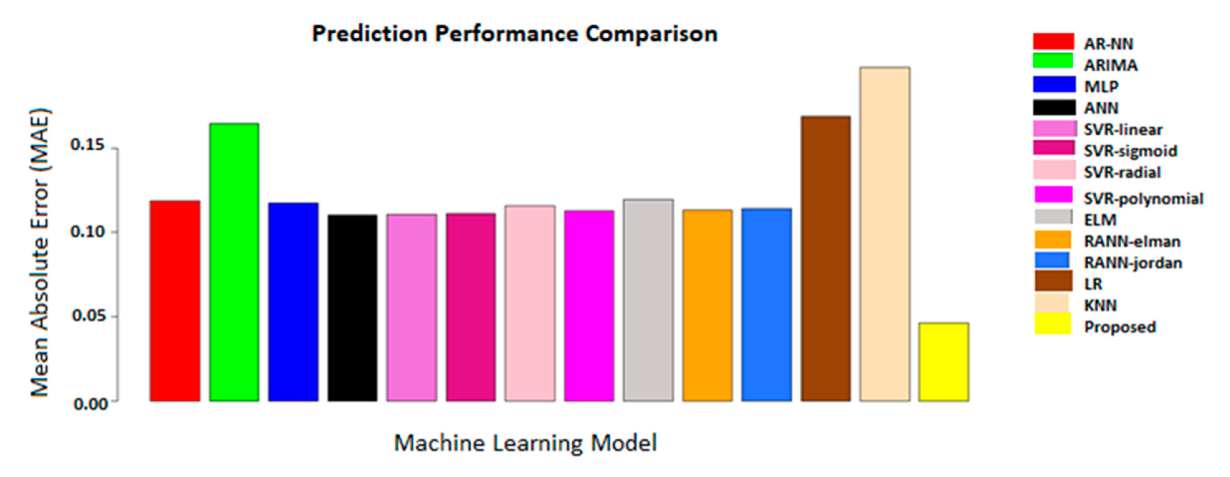
| Model | Type/Characteristics | Space Complexity | Time Complexity | MAE |
|---|---|---|---|---|
| AR-NN | Univariate/hybrid, no built-in window | O(1) | O(1) | 0.11874602 |
| ARIMA | Univariate/parametric, no built-in window | O(1) | O(1) | 0.16476377 |
| MLP | Multivariate/non-parametric, no built-in window | O(1) | O(1) | 0.1172989 |
| ANN | Multivariate/non-parametric, no built-in window | O(1) | O(1) | 0.1100977 |
| SVR-linear | Epsilon with linear kernel, no built-in window | O(n2) | O(n2) | 0.1108303 |
| SVR-sigmoid | Epsilon with the sigmoid kernel, no built-in window | O(n2) | O(n2) | 0.1112155 |
| SVR-radial | Epsilon with the radial kernel, no built-in window | O(n2) | O(n2) | 0.1158454 |
| SVR-polynomial | Epsilon with the polynomial kernel, no built-in window | O(n2) | O(n2) | 0.1127533 |
| ELM | No built-in window | O(1) | O(1) | 0.1193865 |
| RNN-Elman | Elman, no built-in window | O(1) | O(1) | 0.1133194 |
| RNN-Jordan | Jordan, no built-in window | O(1) | O(1) | 0.1139574 |
| LR | No built-in window | O(1) | O(1) | 0.1690222 |
| KNN | No built-in window | O) | O) | 0.1978246 |
| Proposed model | Built-in window | O(1) | O(1) | 0.046356 |
Publisher’s Note: MDPI stays neutral with regard to jurisdictional claims in published maps and institutional affiliations. |
© 2021 by the authors. Licensee MDPI, Basel, Switzerland. This article is an open access article distributed under the terms and conditions of the Creative Commons Attribution (CC BY) license (http://creativecommons.org/licenses/by/4.0/).
Share and Cite
Ullah, Q.Z.; Khan, G.M.; Hassan, S.; Iqbal, A.; Ullah, F.; Kwak, K.S. A Cartesian Genetic Programming Based Parallel Neuroevolutionary Model for Cloud Server’s CPU Usage Prediction. Electronics 2021, 10, 67. https://doi.org/10.3390/electronics10010067
Ullah QZ, Khan GM, Hassan S, Iqbal A, Ullah F, Kwak KS. A Cartesian Genetic Programming Based Parallel Neuroevolutionary Model for Cloud Server’s CPU Usage Prediction. Electronics. 2021; 10(1):67. https://doi.org/10.3390/electronics10010067
Chicago/Turabian StyleUllah, Qazi Zia, Gul Muhammad Khan, Shahzad Hassan, Asif Iqbal, Farman Ullah, and Kyung Sup Kwak. 2021. "A Cartesian Genetic Programming Based Parallel Neuroevolutionary Model for Cloud Server’s CPU Usage Prediction" Electronics 10, no. 1: 67. https://doi.org/10.3390/electronics10010067
APA StyleUllah, Q. Z., Khan, G. M., Hassan, S., Iqbal, A., Ullah, F., & Kwak, K. S. (2021). A Cartesian Genetic Programming Based Parallel Neuroevolutionary Model for Cloud Server’s CPU Usage Prediction. Electronics, 10(1), 67. https://doi.org/10.3390/electronics10010067