A Machine Learning Approach for 5G SINR Prediction

Abstract

Artificial Intelligence (AI) and Machine Learning (ML) are envisaged to play key roles in 5G networks. Efficient radio resource management is of paramount importance for network operators. With the advent of newer technologies, infrastructure, and plans, spending significant radio resources on estimating channel conditions in mobile networks poses a challenge. Automating the process of predicting channel conditions can efficiently utilize resources. To this point, we propose an ML-based technique, i.e., an Artificial Neural Network (ANN) for predicting SINR (Signal-to-Interference-and-Noise-Ratio) in order to mitigate the radio resource usage in mobile networks. Radio resource scheduling is generally achieved on the basis of estimated channel conditions, i.e., SINR with the help of Sounding Reference Signals (SRS). The proposed Non-Linear Auto Regressive External/Exogenous (NARX)-based ANN aims to minimize the rate of sending SRS and achieves an accuracy of R = 0.87. This can lead to vacating up to 4% of the spectrum, improving bandwidth efficiency and decreasing uplink power consumption.

1. Introduction

The use of technology in general and portable devices in particular has skyrocketed in the past two decades. As the technology continues to evolve, various requirements of newly developed standards have emerged, and these requisites have been fulfilled significantly through research and innovation. Wireless and cellular communication technologies have played a vital role in the evolution of technology. Mobile communication marks its birth in the 1970s with the advent of 1G mobile communication systems, which incorporated circuit switching technologies such as Frequency Division Multiple Access (FDMA) along with analog communication techniques. Eventually, the 2G standards evolved with the help of a mechanism where FDMA and Time Division Multiple Access (TDMA) were combined. The first digital communication system designed was 2G [1]. However, the 3G used Code Division Multiple Access (CDMA) and High Speed Packet Access (HSPA) technologies to provide IP- based services in an attempt to meet the demand of higher data rates. In a long Term Evolution (LTE) also termed as 3.9G and LTE-Advanced (LTE-A) also referred to as 4G, incorporate Orthogonal Frequency Division Multiple Access (OFDMA) and Single Carrier Frequency Division Multiple Access (SC-FDMA) in order to achieve much higher rates compared to 3G. Figure 1 shows the evolution from 1G to 5G in terms of services offered.

Figure 1. Evolution from 1G to 5G.

The technological innovation is prospering at an unprecedented rate in the form of Internet-of-Things (IoT), where connectivity is required ubiquitously and pervasively. Ranging from fan to vehicle, CEO to peon, all are required to be in the loop and stay connected to remain up-to-date in the ever changing global technological scenario. Smart homes, cities, cars and industries are envisaged to further soar and toughen the spectrum, speed, QoS (Quality-of-Service) and QoE (Quality-of-Experience) requirements for networks. As per Gartner stats of 2016, 20.4 billion IoT devices are envisaged to be connected by 2020 [2]. The total number of connected devices including IoT devices and mobile devices will reach more than 50 billion by 2021 [3]. IoT devices, scientific research and social media have also resulted in the proliferation of internet traffic leading to an estimate of 2.5 exabytes/day and 40 petabytes/year by CERN’s Large Hadron Collider (LHC) [4]. Considering internet streaming data, approximately 400 h’/min videos are uploaded to YouTube and 2.5 million photos and videos are posted using the platform of Instagram. Consequently, a total of 2.5 quintillion bytes of data are uploaded every day [5]. To cope with all these challenges, the research community is gradually heading towards the next generation 5G network.

Figure 2 shows the journey towards 5G deployment ever since LTE was introduced. Substantial research is going on in the area of mobile communication, which is evident from the number of papers being published in this area. From January 2014 to January 2018, a total of 389 papers have been published in IEEE Xplore, while 588 in ScienceDirect [6].

Figure 2. Plan execution timeline [7].

The 5G is still undergoing standardization and New Radio (NR) was standardized in 3GPP Release 15 [8]. Its requirements include up to 10 Gbps speed and different operating bands (from below 1 GHz up to 100 GHz) of frequency [1,9]. The 5G will inherit several features of legacy 4G system like sub-carrier spacing (with few additional options), Carrier Aggregation (CA) and most of the Reference Signals (RS) [10].

Nevertheless, it is anticipated that 5G will augment some novel and versatile dynamics to networks such as Big Data (BD), Artificial Intelligence (AI) and Machine Learning (ML). AI and ML have evolved as irrefutably important disciplines in the last decade. In the case of 5G, the quality of a network of an operator can be assessed by the quality of deployment of AI techniques [11]. It is making appliances automatic and hence decreasing human intervention, which is also a demand of 5G [12]. In a nutshell, it can be inferred that introduction of AI and its sub-categories in 5G is inevitable [13].

“Spectrum is our invisible infrastructure; it’s the oxygen that sustains our mobile communication”—stated by US Federal Communications Commission Chairman, Julius Genachoeski. It is obvious that spectrum is one of the most precious resources in mobile communication. Therefore, handling spectrum with due attendance is indispensable [14]. In cellular communication, a considerable amount of the spectrum is used for the reference signals. The part of the spectrum that is consumed by the reference signals aggregates up to 25%. Availability of additional spectrum helps in smoothening of the communication. Transmission of these signals adds up overhead as well as consumes a considerable amount of uplink power. In this research, an attempt has been made to save a fraction of the above-mentioned spectrum i.e., 25% mainly utilized by the reference signals. This will help in mitigating the motioned problems.

The recent research advances in Mobile Networks (MN) demonstrates several attempts for saving the spectrum resources as well as power constraints. Some of the researchers are focusing on ML and AI techniques to achieve the said goal. The individual proposed solutions in the literature are orchestrated to address a particular/single problem at a time. As discussed in the literature survey section in detail, the proposed solutions are not multifarious and do not present a single solution for the stated problems. Hence, an efficient technique is required, which addresses the spectrum as well as power usage problems simultaneously.

In this paper, we present a novel method for predicting Signal-to-Interference-and-Noise-Ratio (SINR) based on the location of a Cyber Physical System (CPS). An Artificial Neural Network (ANN)-based model predicts the channel condition, i.e., SINR on the basis of current location of CPS. The Base Station (BS) sends the location in the form of different signals including Position Reference Signal (PRS) and Observed Time Difference of Arrival (OTDoA). In terms of ML, the model has shown good enough (R = 0.87 and MSE = 12.88) accuracy. Furthermore, employing such an approach into the cellular network has contributed in:

• Increased throughput of up to 1.4 Mbps in the case of 16 QAM (Quadrature Amplitude Modulation) and 2.1 Mbps in the case of 64 QAM.
• Saved power of 6.2 dBm at the CPS end.
• Increased bandwidth (BW) efficiency i.e., approximately equal to 4% by saving the fraction of spectrum that is used for the frequent transmission of Sounding Reference Signals (SRS).

The rest of the paper is organized as follows: Section 2 covers the background, Section 3 discusses the literature survey on the use of AI in wireless and cellular networks, and Section 4 is about data collection. In Section 5, simulation setup for data acquisition has been discussed, Section 6 discusses training and testing process for ANN, Section 7 demonstrates the way ANN-based model will be incorporated into MN, Section 8 shows results of the ML model, Section 9 discusses contributions of the proposed scheme and Section 10 provides a conclusion of the discussion.

2. Background

As already discussed, this paper combines two diverse fields of computers, i.e., MN and ML. The framework is conceptually divided into two sections for better understanding of the proposed scheme: (a) Network module (b) ML module.

2.1. Network Module

Mobile communication systems have made a lot of things easier for people, but then, on the other hand, they have posed some tough research questions as well. QoS provision and efficient spectrum utilization are extremely important in mobile communication systems. QoS provision usually relies on proper resource allocation. The spectrum is generally allocated on the basis of channel conditions of CPS users. The channel conditions depend on SINR of the CPS.

For resource scheduling in LTE, an uplink SRS (Sounding Reference Signal) is sent, which intends to estimate channel conditions at different frequencies. 5G will also follow the same pattern except that its SRS will be one, two or four symbols long in the time domain [15]. These SRS are generated on the basis of the Zadoff–Chu sequence [16]. An SRS when received at BS is used to estimate SINR using different state-of-the-art techniques, one such novel method is discussed in [17]. Here is how SRS sequence works mathematically:

$$r_{u,v}^{\alpha }=e^{\mathrm{j}\mathsf{\alpha }\mathrm{n}}{\overline{r}}_{u,v}(n),0\le n\le M_{SC}^{RS}-1$$

(1)

In the above equation, $M_{SC}^{RS}$ represents length of the reference signal sequence and ${\overline{r}}_{u,v}\left(n\right)$ is generated using the Zadoff-Chu sequence and has Constant Amplitude Zero Autocorrelation (CAZAC) characteristics and hence allows orthogonal code multiplexing by cyclic shift $\alpha$, where $\alpha$ is demonstrated as follows,

$$\mathsf{\alpha } = 2\mathsf{\pi }\frac{n_{SRS}^{CS}}{8} (n = 0,1,2,3,4,5,6,7),$$

(2)

Here, $n$ shows the number of SC-FDMA symbols used in uplink. The two indices $CS$ and $SRS$ refer to Cyclic Shift and Sounding Reference Signal, respectively.

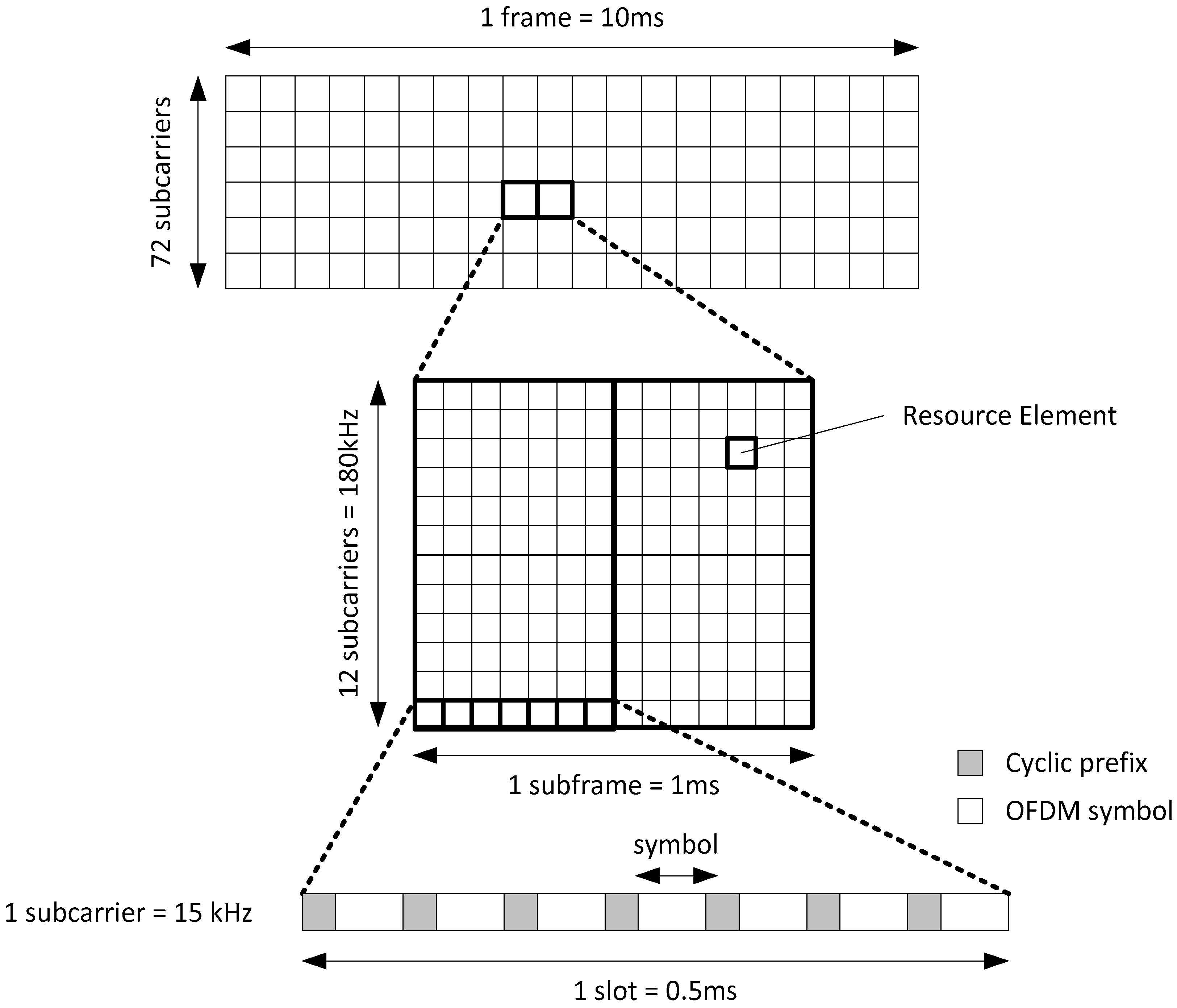
Radio resource scheduling is then done on the basis of this calculated SINR. 5G will also be using the same configurations and features as that of LTE SRS [16] and 5G is also envisaged to give a further role of MIMO configuration to SRS [18]. SRS is sent in gaps of milliseconds. It can be sent as frequently as after 2 ms and as seldom as after 160 ms [16]. Figure 3 shows resource grid of LTE-A. LTE-A and 5G have the same numerology except that the subcarrier in 5G can be up to 30, 60 and 120 KHz and 5G can also have up to 275 PRBs (Physical Resource Blocks) in its resource grid. Different terminologies are explained in Figure 3. Figure 4 shows SRS configuration on a resource grid. It is evident from the aforementioned figures that SRS uses large bandwidth and occupies almost 4.1% of the spectrum. However, in some cases like high Path Loss (PL) and fast fading, SRS may have poor performance on consecutive frequency resources [16]. Frequency hopping is used to overcome this problem.

Figure 3. Resource grid [19].

Figure 4. Sounding Reference Signals (SRS) configuration on a subframe [16].

A Base Station (BS) also acquires a CPS location information using Observed Time Difference of Arrival (OTDOA), Positioning Reference Signal (PRS) or Global Positioning System (GPS) [20]. For the purpose of simulating our network and acquiring required parameters, a Vienna Simulator [21] has been used, while for the purpose of mobility of CPSs, a Random Waypoint model has been used [22].

2.2. ML Module

As already discussed, ML has revolutionized several research areas. It may hardly have left any area of the digital world uninfluenced. Recently, the research area of ML is proving to be of great significance in numerous fields. It is achieving popularity in fields like image processing, medical diagnostics, self-driving cars, etc. With the advent of ML, devices or things are becoming automated, requiring less labor and hence less manual control is needed. In some cases, ML is also proving to be more efficient and reliable than statistical methods [13].

Several techniques with a lot of innovations and revamps have so far been employed for accomplishing AI and ML tasks. However, there is a generic categorization of ML algorithms:

2.2.1. Supervised Learning

It is the category of ML algorithms that works on such data that are pre-labeled. This means that there are pre-defined inputs, we call features, and pre-defined output(s) for them called label(s). Cases where data are continuous and do not belong to a few classes, falls under regression. When the output label is/are discrete class (es) then it is classification.

2.2.2. Unsupervised Learning

These types of algorithms use unlabeled data. These models work in a way that they first learn features from the fed data and then the validation step is done, and after that, data are tested for the already learned features.

2.2.3. Semi-Supervised Learning

It is a kind of hybrid algorithm of supervised and unsupervised algorithms where the data are a mix of labeled and unlabeled data.

2.2.4. Reinforcement Learning

In reinforcement, self-learning behavior of humans and animals is co-opted. It works on the principle of “Action and Punishment”.

2.2.5. Artificial Neural Networks

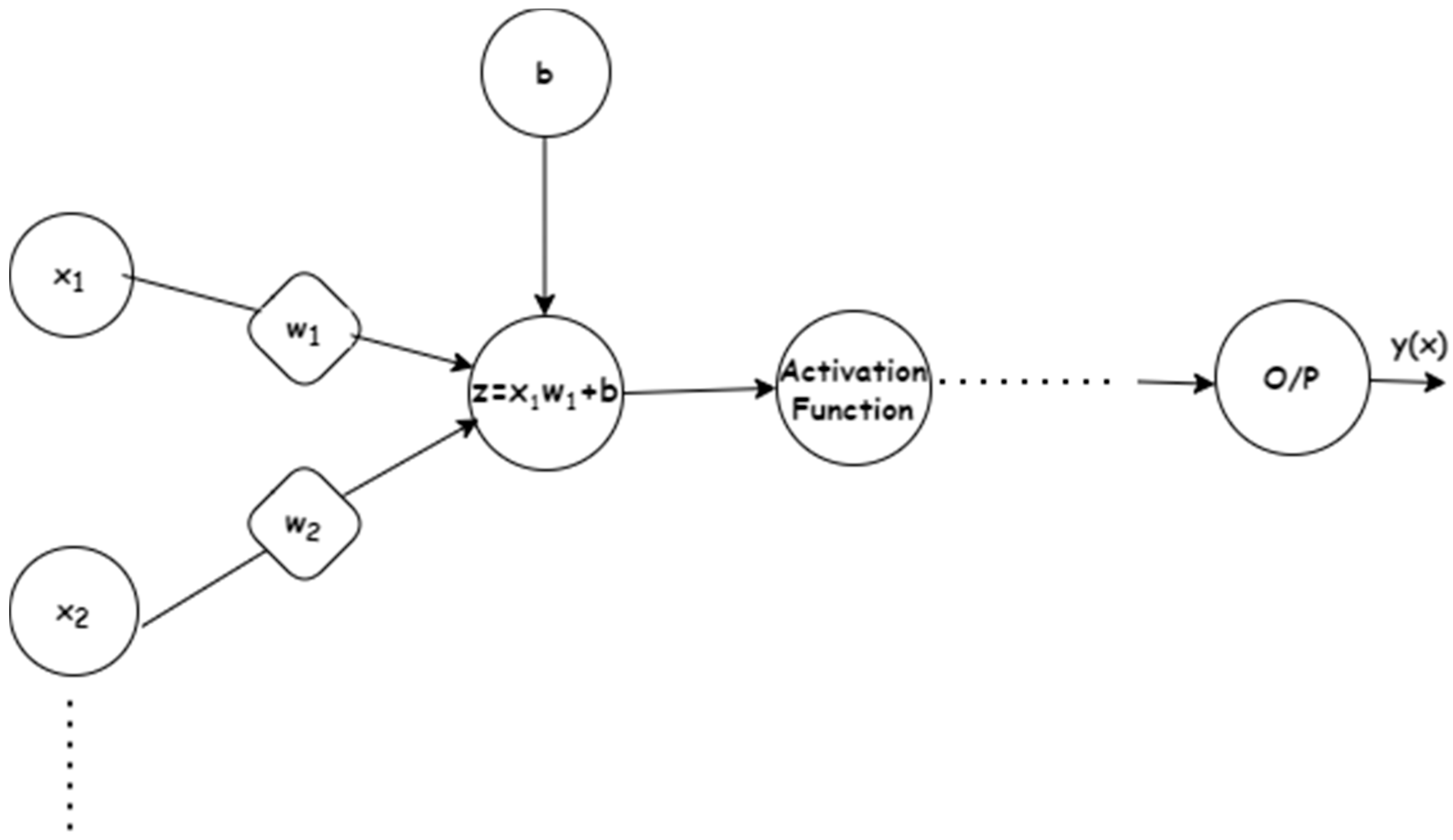
Artificial Neural Networks (ANNs) work on the principle of Human Neural Networks (HNNs). They have certain inputs, multiplied with weights and passed through an activation function for one or more hidden layers and hence reach the output layer. In the O/P layer, results are compared to targets and error is rectified through back propagation for defined epochs and in the last accuracy with best adjusted weight is calculated. A simple ANN is shown in Figure 5.

Figure 5. A simple Artificial Neural Networks (ANN).

Commonly used algorithms in wireless networks are Deep Learning, Ensemble Learning and K-Nearest Neighbors [13,23,24].

An MIT Review has traced the trails of research papers published at arXive.org since 1993. Their findings show the fact that the number of research papers published at arXive.org in this decade has increased more than two-fold as vis-à-vis the last decade [25].

However, neural networks have gained a lot more popularity than other ML algorithms. An MIT review has analyzed research articles of arXive since 1993 of how ANNs have gained popularity especially in the last half of the current decade [25].

For this research work, ANN with a Levenberg–Marquardt algorithm (LBM) has been taken into consideration. An ANN with LBM was selected on the basis of non-linearity of data as ANN and LBM processes and optimizes non-linear data. LBM is the training/ optimization algorithm for ANN to minimize the error. ANN has an input layer that takes the input, multiplies weights to the input, adds bias, and processes it through neurons. The result(s) acts as input to the next layer of neurons. The output layer retracts the values back again for optimization. Here is how it happens mathematically:

$$z={\displaystyle \sum }_{i=1}^n\left(\left(x_i\right)\left(w_i\right)\right)+b$$

(3)

where, $x_i$ is input, $w_i$ is weight and $\mathrm{b}$ is bias.

$z$ is then passed through a squashing/activation function, in our case, for hidden layers, we have used the Sigmoid function also known as logistic function. Mathematically it is shown as follows:

$$y = \frac{1}{{1+e}^{-z}}$$

(4)

For the output layer, a linear function has been used. Mathematically, it is shown as follows:

$$y = cx,$$

(5)

In the above equation, $x$ is the input from the preceding layer and $c$ is the constant.

Optimization is followed with LBM as follows:

$$\left(J^{t}J+\lambda I\right)\delta =J^{t}E,$$

(6)

where $J$ is the Jacobian matrix, $\lambda$ is Levenberg’s damping factor,$\delta$ is the weight update while $E$ is the error matrix.

3. Related Work

Significant research has been carried out so far in wireless networks integration with ML methods and a lot of work is still going on. Here, a few selected pieces of work on ML integration with wireless networks that have been discussed in the research community are revisited.

K. Saija et al. [26] have investigated the delay DL-only (Downlink only) CSI-RS (Channel State Information- Reference Signal). The authors have tried to mitigate the long delay of CSI feedback. A BS transmits CSI-RS in the DL and then the UE sends feedback of this CSI-RS in the uplink to the BS. Authors have considered three ML approaches for building their research, Batch Learning, Online Learning, and Deep Learning. The features they have used are time and SNR while the target output they have considered is CQI (Channel Quality Indicator) and for a part of the experiment they also have added SNR as a target. The ML performance measure they have considered is accuracy improvement of SNR prediction and the network performance has been measured in terms of error mitigation of SNR calculation.

F. D. Calabrese et al. [27] have discussed the problems and opportunities in ML based Radio Resource Management (RRM). The authors have considered two different ML approaches, namely Reinforcement Learning (RL) and Artificial Neural Networks (ANN). In this research, the authors have proposed an architecture for training and learning of ML models for 5G networks. The authors have focused on different RRM parameter predictions like power control, cell and BW, etc.

M. Chen et al. [23] have investigated the issue of spectrum management and multiple access technologies. The authors have adopted an ANN model for resource management. The network condition has been used as input to the model frequency bands as target. This model also has the capability of switching among different frequency bands, which will be a key feature of 5G networks. The task of switching among different frequency bands is based on the availability of Line of Sight (LoS) and congestion avoidance.

D. Kumar et al. [28] have dealt with the upper layers functionalities of an OSI (Open System International) model. The authors have proposed an ML model at the top of HTTP (Hyper Text Transfer Protocol) that would ensure fast and smooth transmission of video data. The authors have proposed an unsupervised (clustering) model. With the said model they were able to achieve up to 7% improvement in peak signal-to-noise-ratio and up to 25% improvement in video quality metrics. The model performance was validated in a live video streaming session.

P. Casas [24] in his research has addressed a couple of smart phone traffic specific problems. The first problem the author has addressed is detecting anomalies generated by smartphones as a result of a large number of data traffic being generated by apps. The other problem addressed is the prediction of Quality-of-Experience (QoE) for the most used apps. An Ensemble Learning (EL) model has been preferred where six different algorithms have been ensembled. The ensembled algorithms are decision trees, Naïve Bayes, Multi Layers Perceptron (MLP), Support Vector Machines (SVM), Random Forests (RF) and K Nearest Neighbors (K-NN). In this research, the authors have achieved an accuracy of up to 99% using EL stacking.

Some other issues addressed by researchers in this field are as follows:

• Handover prediction [29];
• Link status prediction [29];
• Intrusion detection system [29];
• Modulation classification [30];
• Network optimization using different techniques [30];
• QoE enhancement for 5G [31];
• AI as Micro Service (AIMS) for data-driven intelligent traffic over 5G networks [32];
• Cognitive autonomous 5G networks [33];
• Wireless network monitoring and analysis [24];
• Fault Diagnosis for autonomous vehicles using SVM [34].

It can safely be pronounced that several problems/issues regarding ML integration with wireless networks have been addressed but still there is a huge gap to be addressed. ML is anticipated to play a key role in 5G and later systems. Hence, there is a dire need of this area to be addressed. Here are some opportunities, for mobile and wireless networks in general and 5G in specific, described in literature:

• Accurate channel state information estimation [35];
• Network optimization modeling [35];
• Approaches to select best (less complex) machine learning algorithms for wireless networks [13];
• Network resource allocation is attributed to be one of the key issues in 5G [35];
• Spatio-temporal mobile data mining [13].

There are a handful of research gaps in 5G for AI and ML, albeit, there are many more opportunities being discussed in the literature as in [13,23,29]. Table 1 gives an insight of AI integration into MN and why they could not solve the problem.

Table 1. A glimpse of the literature survey.

Reference	Problem(s) Addressed	Power Saving	Throughput Increase	BW Efficiency	AI Integration
[36]	Power saving at user end	Yes	No	No	Yes
[37]	Saving Power at BS	Yes	No	No	Yes
[38]	Increased capacity with optimized power	Yes	No	Yes	No
[39]	Resource allocation for NOMA	Yes	No	Yes	No
[40]	Power optimization	Yes	No	No	No

4. Data Acquisition

As a rule of thumb for ML algorithms, they need data for training, which includes features and labels (in case of supervised learning). In our case, features are geographical positions of the user, i.e., X and Y coordinates and the labels are the SINR values. To acquire SINR, MATLAB based traces from a Vienna simulator are obtained and a Random Waypoint mobility model is simulated for 10,000 s to get the mobility patterns, returning almost 200,000 instances of SINR against X, Y coordinates. These traces were acquired for a single node. The speed interval of the node was set to 0.02 m/s and the pause interval was 0 s (no pause). The time step for trace collection was 0.001 s. 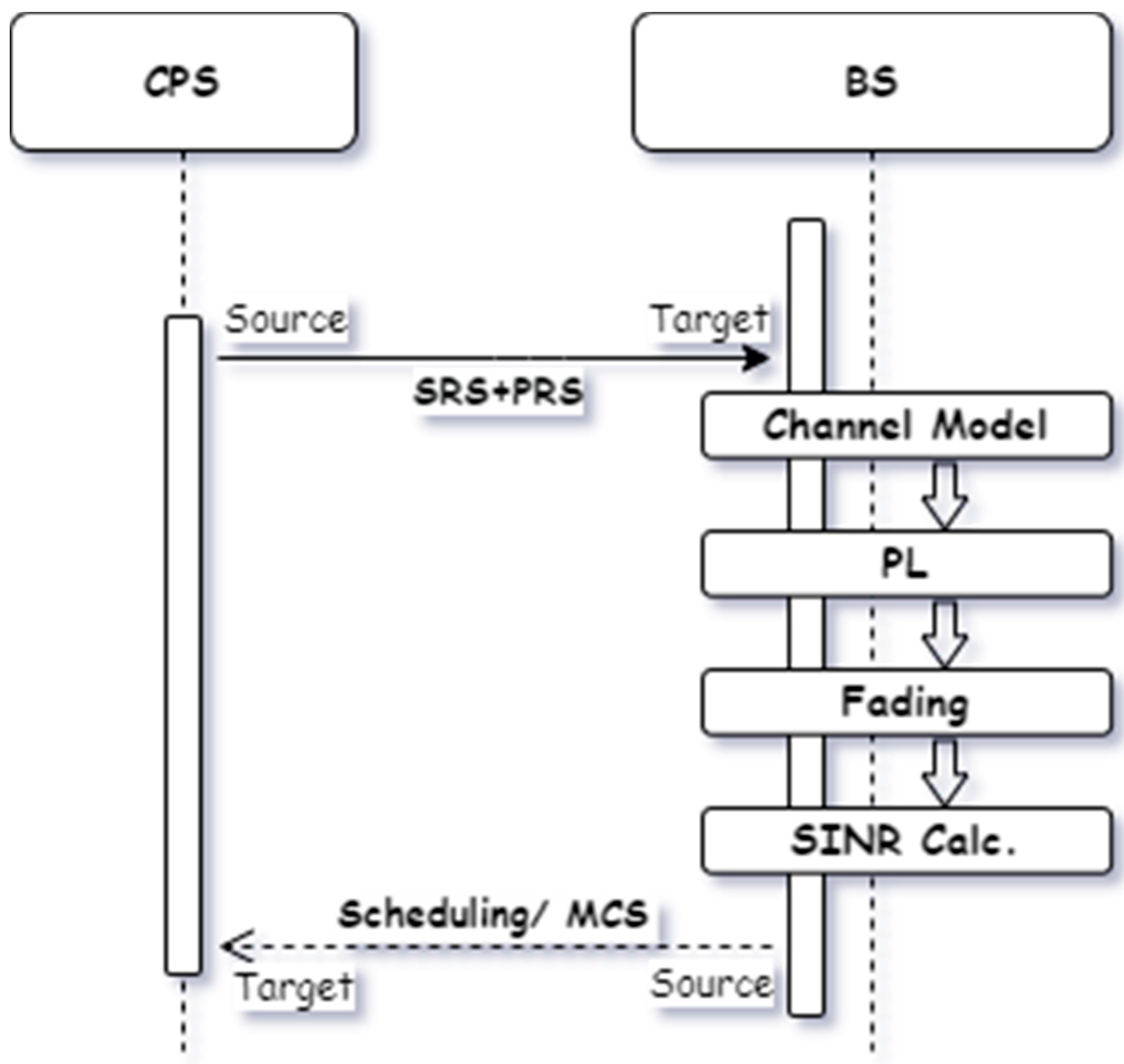Figure 6 shows the simulation process of how data are collected. Where a CPS sends SRS and position signal to a BS and BS estimates SINR from that, and then allocates the scheduling scheme accordingly.

Figure 6. Data acquisition.

5. Simulation Setup

The footprints of channel conditions were obtained using a Vienna simulator. A MATLAB-based system level simulator was developed for simulating advanced networks. In order to obtain the link quality (i.e., SINR), the model uses three parameters. The first parameter is the Macro path-loss (L), which models both L due to distance and antenna gain. Distance based L is calculated using the following formula.

$$L = 128.1 + 37.6\mathit{log}{}_{10}R \left[\mathrm{Km}\right]$$

(7)

In the above equation, $R \left[\mathrm{Km}\right]$ represents the distance between transmitter and receiver in kilometers, whereas $128.1$ is a constant and $37.6$ is the constant coefficient of the second term in the equation.

The second parameter is the shadow fading, which estimates the loss of the signal due to obstacles in the way of signal traveling from transmitter to receiver. It is referred to as the introduction change in geographical properties with respect to the Macro path-loss. The third parameter is channel modeling. In this part, J. C. Ikuno et al. [41] have considered small scale fading as a time varying function. Channels have been modeled for both multiple-input and multiple-output (MIMO) and single-input and single-output (SISO) modes of transmission. Finally, the link quality traces are collected from the Vienna simulator. Different scenarios have different SINR estimation methods. Our SINR of interest uses SISO as the uplink. Systems such as LTE have only SISO support, but the model could be extended to MIMO as well. SISO-based SINR is estimated using the following formula.

$$\mathrm{SINR}=\frac{P_{tx}}{\frac{1}{{\left|h_0\right|}^2}{\sigma }^2+{{\displaystyle \sum }}_{i=1}^{N_{int}}\frac{{\left|h_1\right|}^2}{{\left|h_0\right|}^2}{P}_{tx,i}}$$

(8)

where $P_{tx}$ is the transmission power, $\frac{1}{{\left|h_0\right|}^2}, \frac{{\left|h_1\right|}^2}{{\left|h_0\right|}^2}$ are noise and interference traces, $P_{tx,i}$ shows transmission power at the $i^{th}$ transmitter.

6. Training and Testing

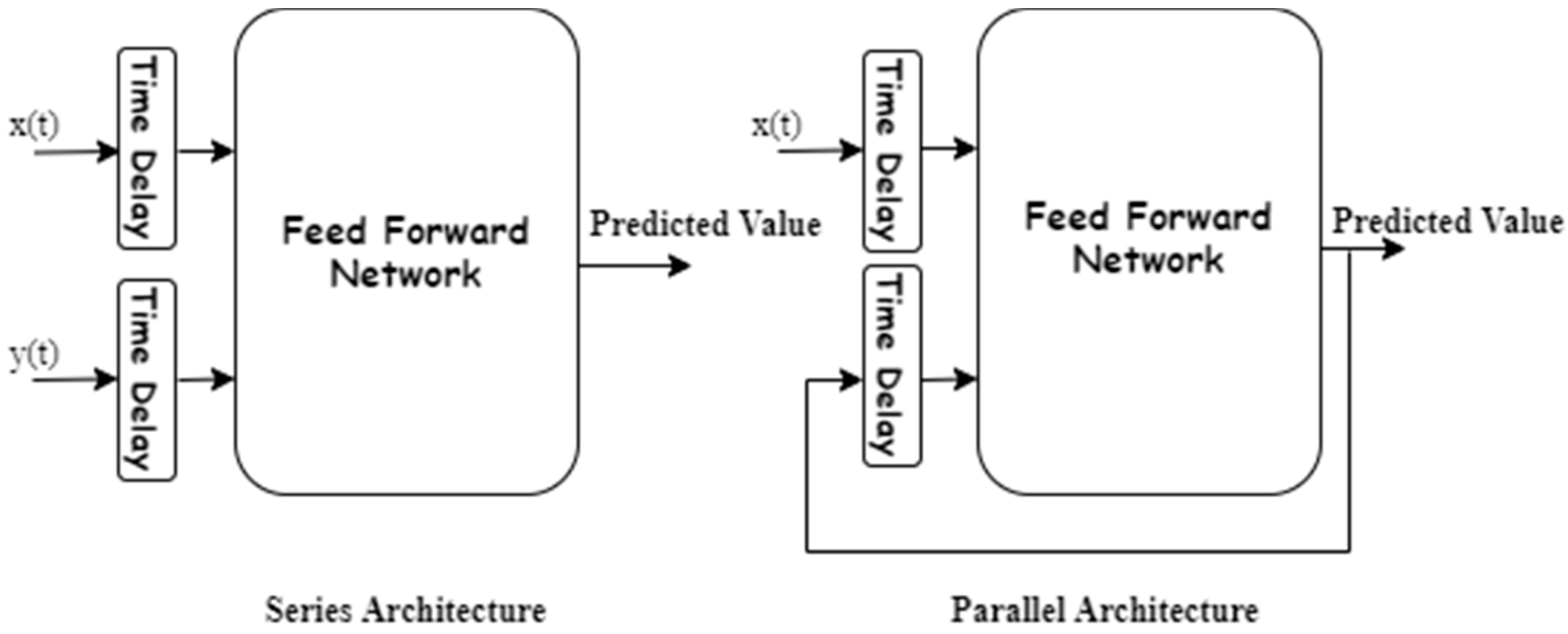
As it has already been discussed, the acquired dataset has two input features, i.e., the coordinates of the user location and the SINR. So, in light of the available data, our problem lies in the scope of supervised learning. As the output label is a vector of continuous values of SINR, the regression technique has been used for curve fitting. The MATLAB environment is used for the experiment. The ANN model that has been used for this experiment is a Non-Linear Auto Regressive External/Exogenous (NARX) model. The NARX model has two architectures—one is series-parallel architecture, which is also called an open-loop and the other is a parallel architecture also referred to as closed loop. We preferred the open loop architecture for our simulations mainly because the true output is provided to the network, unlike a closed loop that feeds an estimated output. Another advantage of using an open loop is that it uses a simple feed forward network, which allows to incorporate efficient training algorithms [42]. The two different architectures of NARX are depicted in Figure 7.

Figure 7. Non-Linear Auto Regressive External/Exogenous (NARX) [42].

Mathematically, open loop NARX is shown by the following formula:

$$\widehat{y}(t)=f\left(y(t-1),y(t-2),\dots ,y\left(t-n_y\right),x(t-1),x(t-2),\dots ,x\left(t-n_x\right)\right),$$

(9)

In the above equation, $\widehat{y}\left(t\right)$ is the predicted value based on the previous value of the input vector $u(t-1)$ as well as that of the output vector $y(t-1)$. $F(.)$ is the mapping function, $n_y$ represents output delays, while $n_x$ shows input delays.

Results show that the best performance/accuracy ($R=0.87112$) is achieved when the training data are spread across the time domain. The spreading of data in the time domain means that the input data are not fed at once along with the delays.

The dataset is split into three sets including training, validation and testing in the proportion as shown by Table 2. The configuration of the proposed neural network comprises 15 hidden layers with 5 delays and 20 epochs. The results show that the training process stops if the generalization, i.e., cross validation does not improve beyond six iterations.

Table 2. Distribution of the dataset.

Dataset	Proportion
Training	70%
Validation	15%
Testing	15%

7. Working

Initially, it is not desired to totally exterminate the SRS; nonetheless, the goal is to reduce its transmission rate by half. As already discussed, SRS is normally transmitted after every 2 ms, but because of this experiment it is transmitted after 4 ms and for the rest of the 2 ms, BS predicts SRS based values of SINR with the trained ML algorithm.

Normally, a regular communication of SRS and geo-position signals between the user and BS exists. In this case, it is proposed to reduce the rate of the communication of SRS to half. In the deployed systems, SRS is transmitted almost after every 2 ms and it is proposed to send SRS after 4 ms in order to save two sub frames, which are especially configured for SRS. The CPS regularly communicates its position to the BS in the form of PRS.

In the 2 ms of the middle, where no SRS is being communicated, ML helps in predicting the channel conditions. In this case, only the position signal is to be configured for transmission on the basis of geo-location of the CPS. Since the machine has been trained for predicting SINR, BS schedules DL resources for the CPS without SRS being transmitted. Figure 8 shows this concept through a flowchart.

Figure 8. Flow chart for implementation of the proposed scheme.

It is inferable from Figure 8 that first the CPS will be configured in such a manner that it will decide whether to use ML or the classical statistical method. If it is ML’s turn, then the CPS sends only its position signal rather than sending SRS and at the BS the position coordinates are provided to the ML model in order to predict the SINR. DL scheduling is decided on the basis of the calculated SINR.

Alternatively, if it is not ML’s turn, then the CPS will send SRS as well as position signal to the BS. The BS will estimate SINR on the basis of the received SRS (already discussed in Section 2). Therefore, the scheduling is achieved based on this estimated SINR.

For the decision of when it will be the turn of the ML model calling and the classical method calling, we proposed the following Algorithm 1.

Algorithm 1: Method decision

start              for t equals 0 to_max with t + 2ms                            {                            CPS.Classical_Method                            }              for t equals 1 to_max with t + 2ms                            {                            CPS.ML_Method                            } end

The BS configures a CPS on the basis of the above algorithm. For the time slot ($t=0$), the classical method is called where both SRS as well as position signals are transmitted. For the next slot, the ML method is invoked and only a position signal is being sent and an ML model is applied.

Here, only the time domain is taken into account due to the fact that the already proposed/allocated bandwidth for SRS is not being decreased but in fact its transmission in the time domain is intended to be decreased. SRS will still stretch over a large bandwidth but not as frequent in time as it used to be previously.

8. Results

After completing the training, validation and testing task, different matrices of performance measurement are acquired. However, the parameter considered here is the loss function and accuracy measure obtained at the end of the simulation. The loss function preferred for our experiment is Mean Squared Error (MSE) and the accuracy measure is Regression (R). The MSE achieves a value of 12.88 and the accuracy measure of the experiment is 0.87, as shown in Figure 9. Mathematically, MSE works as follows:

$$\mathrm{MSE}=\frac{1}{n}{\displaystyle \sum }_{i=1}^n{\left(y_i-{\tilde{y}}_i\right)}^2$$

(10)

Here, $y_i$ shows target/real output, while ${\tilde{y}}_i$ is the predicted/ estimated output.

Figure 9. Machine Learning (ML) model accuracy.

The mathematical formula of R is as follows.

$$\mathrm{R}=\sqrt{\frac{{{\displaystyle \sum }}_{i=1}^n{\left({\tilde{y}}_i-\overline{y}\right)}^2}{{{\displaystyle \sum }}_{i=1}^n{\left(y_i-\overline{y}\right)}^2}}$$

(11)

The $\overline{y}$ in above equation shows mean value of ${\tilde{y}}_i$.

There are four different results in Figure 9 obtained at different stages of the experiment. Overall, this figure shows the comparison of the real output (target) with the predicted values (output). The training results are those that have been obtained during the training phase. The model achieves an accuracy of 0.87 for training. The validation results are obtained during the validation step (ensuring that there is no overfitting) and yielded an accuracy of 0.86. The testing results are those obtained after feeding the test part of the dataset. Accuracy of the test phase is 0.86. The last result shows a generic model obtained after running all of the above steps. $Output=0.77\times Target+1.7$ is the final model obtained, it shows that the input ($f\left(y,x\right)$) is multiplied with the coefficient 0.77 (weight) and then added with 1.7 (bias). The fit and Y = T lines show the convergence of the real output and target and the data legend shows the distribution of data instances against the fitness function.

Table 3 shows a comparison of accuracy of NARX with a Non-Linear Input Output technique and SVM with 10-fold cross validation under R accuracy measure and for the same data. It can be inferred that NARX outperforms the latter.

Table 3. Comparison of accuracy of NARX with Non-Linear Input Output and Support Vector Machines (SVM).

Model	Accuracy
NARX	0.87
Non-Linear Input Output	0.79
SVM	0.47

Equation (12) shows how the Non-Linear Input Output technique works mathematically.

$$\widehat{y}(t)=f(x(t-1),\dots ,x(t-d))$$

(12)

Table 4 shows performance parameters at a glance. The RMSE (Root MSE) is acquired by taking the square root of MSE. The r² shows the R-squared value that has been acquired by taking the square of the regression value R.

Table 4. Performance measures.

Parameter	Value	Percentage
R	0.87	87%
MSE	12.88	N/A
r²	0.75	75%
RMSE	3.58	N/A

9. Contribution

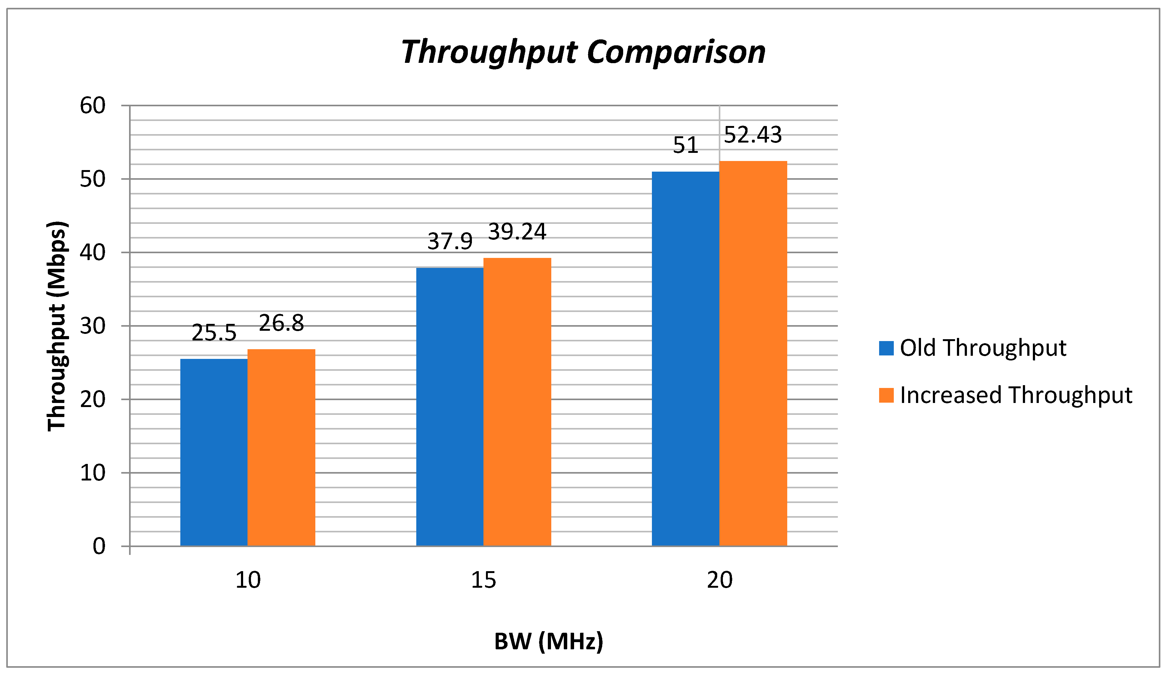
The increase in the amount of maximum throughput/good-put capacity for 16 QAM is depicted in Figure 10. Payload throughput is obtained after the exclusion of reference signals overhead, reference signals take up to 25% of the total capacity of a channel BW. Here, 10 MHz BW may not seem better for some higher frequencies in 5G because it will not satisfy the higher data rate requirements; however, it is still considered by standardizing bodies and operators for Non-Standalone (NSA). NSA is the initial phase of 5G, where it will work as an extension of 4G and will use LTE packet core and lower frequencies in Standalone (SA). SA will be the full fledge 5G system requiring no LTE or LTE-A support [43,44]. For this reason, this paper also considers 10 MHz BW. Besides that, 15 and 20 MHz BW are stronger candidates for uplink in 5G, and therefore considered in this work [45]. 256 QAM and MIMO have not been considered because they are not supported at the CPS.

Figure 10. Throughput comparison for 16 QAM (Quadrature Amplitude Modulation).

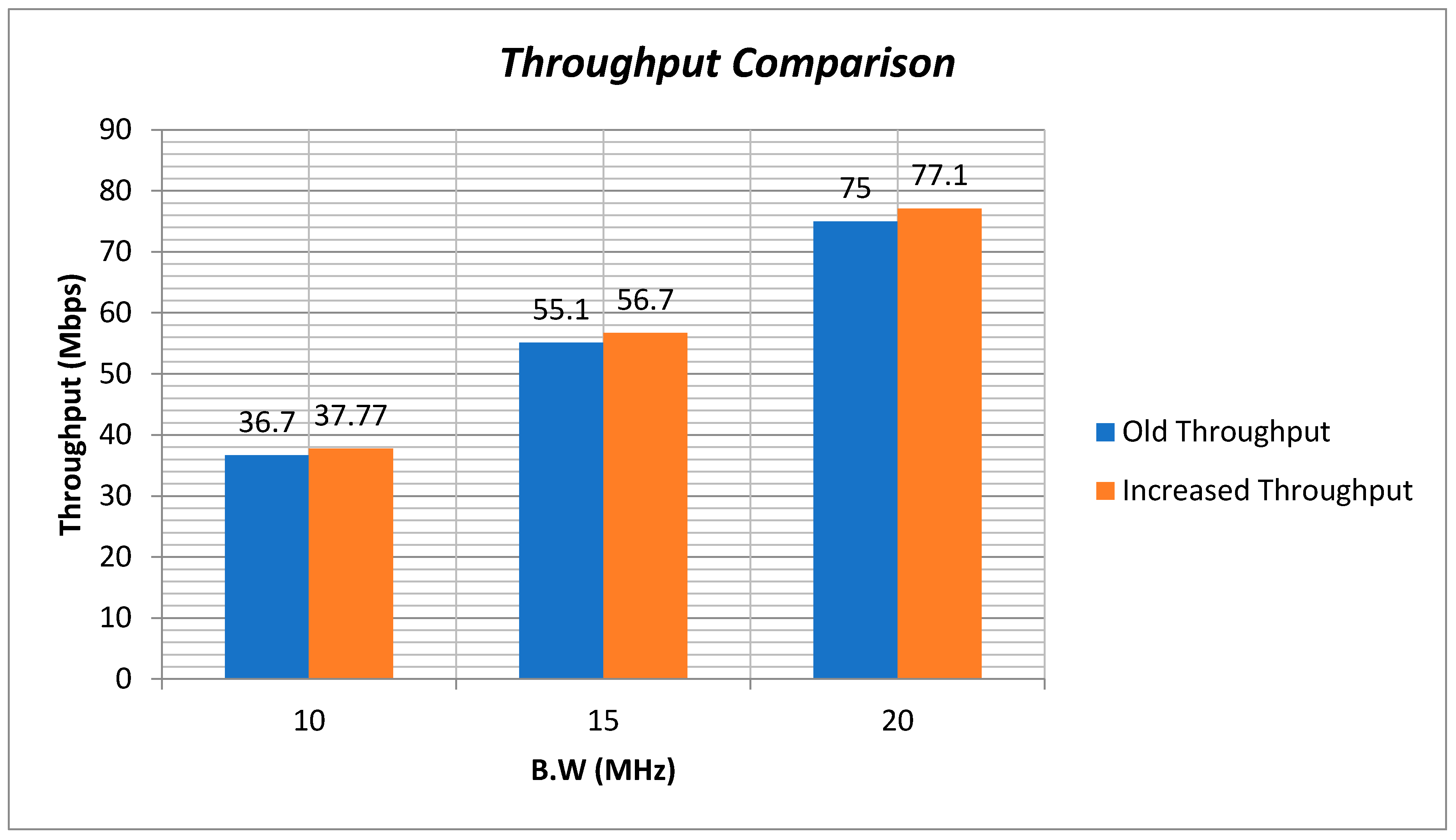
The impact of the proposed mechanism on throughput with 64 QAM scheme, where 6 bits/symbols are allowed is depicted in Figure 11.

Figure 11. Throughput comparison for 64 QAM.

As seen in the results section, the ML model has been trained, now its incorporation into the network allows us to reduce the number of transmissions of SRS. This increases the throughput capacity.

Throughput is the measure of real user data (bits) transfer capacity of a BW in one second. This is acquired by subtracting the overhead from the total capacity of a BW. The increased throughput is obtained by adding the saved part of SRS to the payload/ throughput of the BW.

$$S_{old}=C_{ch}-C_{oh}$$

(13)

Here, $C_{ch}$ is the capacity in bits/sec of a channel for a given BW while $C_{oh}$ is the reference signal overhead capacity in bits/sec and $S_{old}$ is the throughput in bits/sec.

$$S_{new}=S_{old}+C_{SRS}/2$$

(14)

$S_{new}$ is the enhanced throughput. It has been obtained by adding $S_{old}$ and $C_{SRS}/2$. $C_{SRS}/2$ is the channel capacity dedicated for SRS in bits/sec. The 2 in the denominator shows that in the obtained results, SRS transmission has been reduced to half.

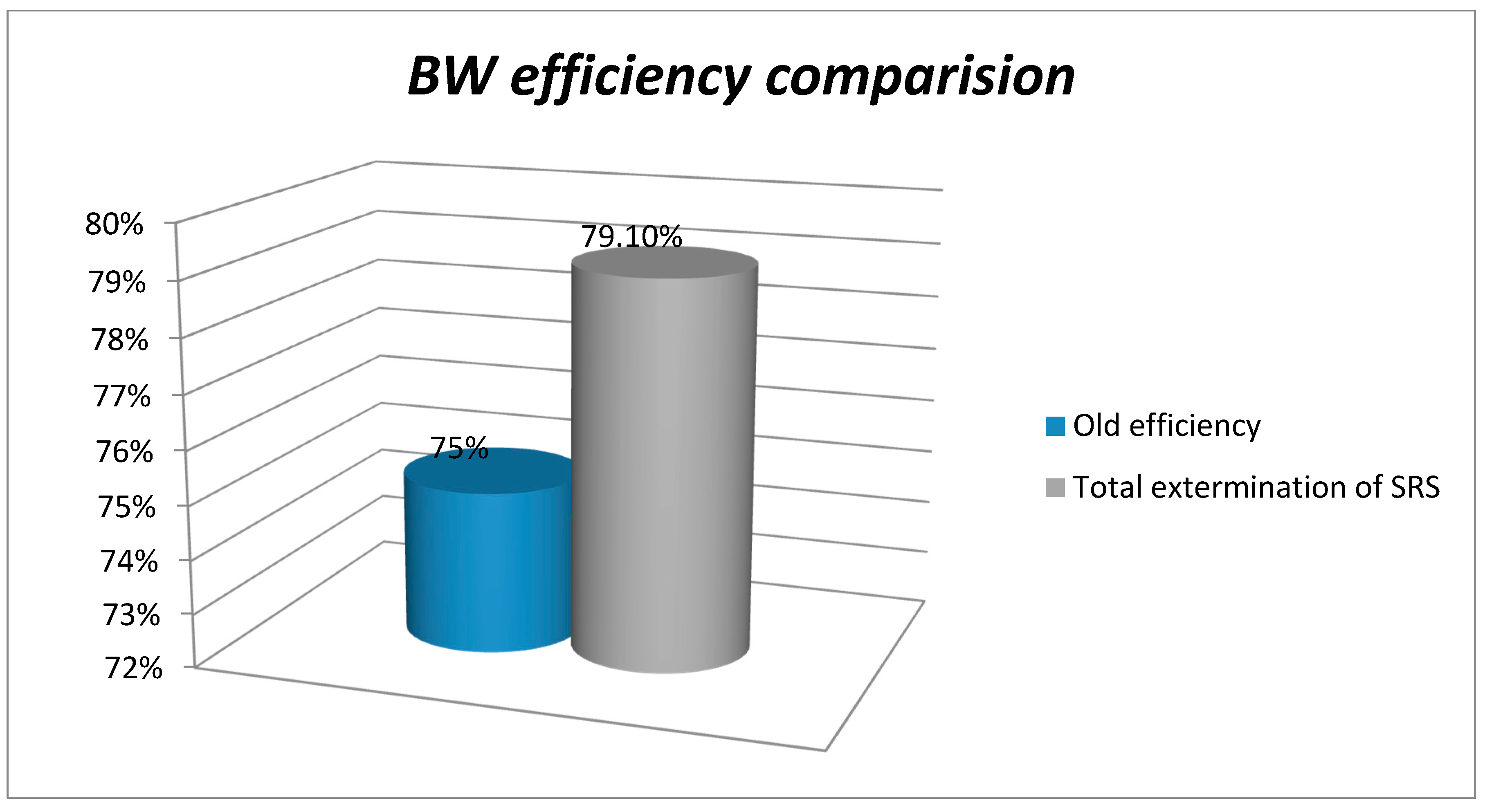
The exclusion of overhead increases the efficiency of BW utilization. Normally, almost 25% of the channel is used for reference signals, for example, SRS, Demodulation Reference Signal (DMRS), overhead and the rest of the 75% is usable for real user data transfer. Among the 25% of the channel BW that is occupied by reference signals, SRS only occupies 4.1% of the BW.

So, in the proposed solution, the BW efficiency for real user data throughput increases by about 2% when SRS transmission is reduced to half and the BW efficiency increases approximately by 4% when SRS transmission is totally replaced by the ML model and hence the total usable part of BW for user data becomes 77% and 79% respectively. Thus, a remarkable BW efficiency improvement can be effectively realized. Figure 12 shows a graphical representation of BW efficiency.

Figure 12. Bandwidth (BW) efficiency.

The typical power consumption for a CPS in uplink is 23 dBm per physical resource block, as per 3 GPP [46]. This becomes 199 mW on a linear scale. Since the number of transmissions of SRS has been significantly reduced, a decrease in power consumption can also be noticed by the same proportion. It saves us power of almost 4.1 mW, which in log scale becomes 6.2 dBm. Hence, useful power can be conserved by consumption reduction.

10. Conclusions

In this paper, a different paradigm is investigated for introducing artificial intelligence in mitigating resource utilization in a physical layer of SRS. We proposed a novel method for predicting an uplink SINR, which is based on SRS using an ANN-based scheme. This research holds potential value for enhancing the most precious aspects of RRM. We attempted to mitigate the research gap by increasing the throughput, saving uplink power, and increasing BW efficiency for 5G networks through prediction rather than estimation via pilot signals. This research is important for exploring new future ideas, such as the prediction of PL, fading, QoS and power control.