How Human Mobility Models Can Help to Deal with COVID-19

Abstract

One of the key factors for the spreading of human infections, such as the COVID-19, is human mobility. There is a huge background of human mobility models developed with the aim of evaluating the performance of mobile computer networks, such as cellular networks, opportunistic networks, etc. In this paper, we propose the use of these models for evaluating the temporal and spatial risk of transmission of the COVID-19 disease. First, we study both pure synthetic model and simulated models based on pedestrian simulators, generated for real urban scenarios such as a square and a subway station. In order to evaluate the risk, two different risks of exposure are defined. The results show that we can obtain not only the temporal risk but also a heat map with the exposure risk in the evaluated scenario. This is particularly interesting for public spaces, where health authorities could make effective risk management plans to reduce the risk of transmission.

1. Introduction

The eruption of the COVID-19 pandemic has become a severe threat to our society and our way of living. For the time being, more than a million people have died, more than 10 million are infected, and the collateral effects of this pandemic are affecting each and every part of our society and economy. There is no sign that its effects will diminish in the short term, as vaccines are still in test stages and it seems that no new effective treatments have emerged.

Other approaches are based on leveraging the increasing availability of data, communications, and computing power. The so-called Digital Epidemiology takes advantage of this technology to track infectious diseases and to allow new approaches to deal with epidemics [1]. Digital Epidemiology is epidemiology that uses data that was generated outside the public health system [2], as for example, mobile phones tracking information, social network tendencies, and mobility models.

For example, contact tracing can be considered a more selective isolation measure targeted to the population most likely to have the infection [1]. The utilisation of current smartphones has led to the creation of what is called smartphone-based contact tracing, which is used to detect the exposure to risky contacts [3,4,5,6]. For example, Apple and Google have recently teamed up to include the necessary support into their smartphone operating systems to implement these applications. Most of the technology of these mobile applications are based on the results of years of research on mobile computing and singularly on Opportunist Networks.

Opportunistic Networks use proximity contacts of mobile devices to exchange messages in a way to spread information among these devices. Their behaviour and dynamics can be comparable to the epidemic spread of a disease, so the models developed to evaluate opportunistic networks are usually adaptations of known epidemic models [7]. The study of human mobility and social behaviour is also essential for evaluating information dissemination in these opportunistic networks [8].

A lot of mobility models have been used for evaluating the transmission of messages in Opportunistic Networks. Much of these models are from related mobile networks, such as Mobile Ad hoc Networking (MANET) and DTN (Delay Tolerant Networks). In current mobile networks, mobility and the number of users in a scenario can vary during the evaluation time, and therefore it is necessary to have scenarios or models that try to reproduce human behaviour as truly as possible.

The general idea of this paper is to evaluate how Opportunistic Networks (OppNets) mobility models can be applied to the fighting against COVID-19. Particularly, these models can be used to evaluate the exposure risk of contagion in a given place. Whereas in OppNets the idea is to evaluate the opportunity of transmitting a message when two mobile devices contacts (that is, there are within communication range), in this paper the idea is to evaluate the opportunity of transmitting an infection when two individuals are close.

COVID-19, the disease, is caused by the SARS-CoV-2, the virus, which is a strain of coronavirus. There is overwhelming evidence that the SARS-CoV-2 virus inhalation represents a major transmission route for COVID-19 [9]. The SARS-CoV-2 virus is transmitted mainly by droplets and aerosols and are highly concentrated near an infected person, so they can infect people more easily in close proximity. The virus transmissibility is also affected by the quality of the medium, i.e. air renewal, temperature, and solar radiation which can reduce their transmission. From the beginning of the COVID-19 pandemic, it was shown that there is a higher risk of transmission indoors compared with outdoor environments [10].

In this paper, we generate several scenarios to evaluate the temporal and spatial risk of being infected. We start with basic synthetic scenarios, such as Random WayPoint Model (RWP), Small World in Motion (SWIM), and Random WayPoint Model with attraction points (RWPa). These models, used often in OppNets evaluation, are shown to be quite unrealistic for evaluating the COVID-19 spread. Therefore, we propose the use of a pedestrian mobility simulator for building realistic scenarios in order to generate people mobility traces. The utilisation of these mobility simulators was originally proposed in [11] for OppNets evaluation. A pedestrian simulator can model the microscopic (individual) and macroscopic (crowd) dynamics of pedestrian mobility, an option that is not supported by the synthetic mobility models [12]. More specifically, we consider a square (particularly, a plaza) and a subway station, which are typically crowded scenarios with a high degree of people renewal. Summing up, the idea is to generate a mobility trace to detect possible contacts and risky spots.

We introduce two methods to evaluate the exposure risk to contagion. The first one is based on the method used by smartphone-based contact tracing applications, considering only the time and distance (a contact is considered risky if two persons are within 2 m for more than 15 min). Since this model does not consider the environment (that is, indoor/outdoor, ventilation etc.), we introduce a new expression where the quality of the medium is determined by the type of scenario and its characteristics.

The evaluation of the scenarios using these models shows that pure synthetic models cannot offer realistic human mobility patterns and therefore the risk maps obtained using these models are not useful. On the contrary, the results obtained using the scenarios generated with the pedestrian simulator are very realistic, and we can obtain spatial heat maps and temporal plots of the exposure risk. Furthermore, using the second method to evaluate the exposure risk, we can verify that outdoor scenarios, such as the plaza, exhibits a very low-risk exposure when compared to indoor scenarios, such as the station. These temporal and spatial maps would allow authorities to take measures to avoid risky spots in order to reduce the transmission of the COVID-19.

The outline of this paper is as follows. Section 2 provides an overview of related works. Section 3 is a short survey of mobility models used in Opportunistic Networks. The generation of the scenarios used in the paper is described in Section 4 which are temporally and spatially evaluated in Section 5. Section 6 analyses how the SARS-CoV-2 is transmitted in order to characterise the exposure risk, which is used in Section 7 to evaluate the risk on the different scenarios. Finally, Section 8 details the main conclusions.

2. Related Work

Surveillance and control of emerging infectious diseases are vital for public health. The utilisation of new technologies, such as internet-based surveillance, infectious diseases modelling, remote sensing, telecommunications, and mobile phones, can predict, prevent, and control these infectious diseases [13]. It is a new approach to deal with epidemics, usually categorised with a newly coined term: Digital Epidemiology [2].

A recent technology which can be used to cope with COVID-19 is Opportunistic Networks (OppNets). OppNets are based on the opportunity of contacts between mobile devices (that is when they are in communication range) as a way to propagate messages. The effectiveness of OppNets depends mainly on users’ mobility. The dependence between mobility and the performance of OppNets have been studied extensively, see for example [7,14,15,16,17]. For example, Garg et. al. [16] studied the impact of node density on the data dissemination time using a synthetic mobility model. Other proposals, such as [18,19], study the message dissemination behaviour of the Epidemic protocol by focusing on the mobility patterns of the nodes, evaluating the relationship between factors such as mobility model, speed and node density, and locations of the nodes. Other papers are more focused on evaluating the impact of human behaviour in the opportunistic forwarding of messages [20,21]. In general, the previous results show that information diffusion increases with the node density and the number of contacts, mobility being the main enabler of opportunistic data dissemination [22].

Since mobility is a key factor for evaluating OppNets, several synthetic models have been devised in order to capture this human mobility. From the basic models, such as Random Walk and Random Waypoint [23], to more realistic models that consider some social aspects of human movements like working days and meal hours. Nevertheless, these synthetic models can only capture some specific characteristics of human mobility.

Therefore, given the limitation of these synthetic models, some recent papers use pedestrian simulators for evaluating the mobility of pedestrians. In [11], the authors introduce a complex model for streets based on queues, along with contact and duration probabilities. This model is compared with simulation results using the commercial pedestrian simulator LEGION. Using this pedestrian simulator, the authors in [8] study the impact of mobility and the scenario used on opportunistic communication (inter-contact time and contact duration). The results show that, as expected, the type of scenario is the most important aspect to consider, and so a general model cannot be derived.

Mobility models and infection dynamics are also related to Network Science, since the transmission of COVID-19 requires a contact or at least proximity, and this is a network of contacts [24]. So, the dynamics of the COVID-19 can be explained using techniques of network science.

Regarding the risk of transmission, it depends on the following factors: contact pattern, host-related infectivity/susceptibility pattern, environment, and socioeconomic status [25]. Early studies of COVID-19 provided evidence that sustained close contact drives the majority of infections. For instance, family/friend gatherings or travelling on public transport were found to have a higher risk for transmission than brief (<10 min) encounters [26,27]. Furthermore, findings from contact tracing studies suggest a higher risk of transmission indoors compared with outdoor environments [10]. That is, prolonged contact in an enclosed setting can lead to increased risk of transmission. Finally, recent studies have focused on evaluating the risk of airborne transmission of SARS-CoV-2 as a function of time using the known Wells–Riley equation [28,29,30,31] or the Drake equation [32].

Recent studies have shown that not only SARS-CoV-2 viruses are transmitted in droplets, which have a reduced lifetime and range (less than 2 m) but also in aerosols, which can remain suspended in air for hours [9] and reach longer distance. Therefore, some considered interpersonal safe distances should be revised.

Several macroscopic models have been proposed to evaluate how different infectious diseases spread across cities, countries, or worldwide, considering geographical and mobility aspects (see for example the spatial models described in [33]). For COVID-19, an interesting model is the one proposed by Sun et al. [34]. Their COSRE risk assessment tool obtains the exposure risk in EE.UU.’s counties (that is, the geographical risk) based on the probability of contacting infected people using the birthday paradox probability and real-time data of the potential COVID-19 cases in the counties. Another interesting macroscopical model is the one proposed in [35]. It is a macroscopical approach using a stochastic SEIR metapopulation model to predict the evolution and spreading of the COVID-19 across the different regions of Spain also using real mobility data.

Finally, some studies have combined the use of mobility traces to evaluate the COVID-19 spread and the risk of transmission. For example, Muller et al. used real mobility traces to evaluate the spreading of the infection in the city of Berlin [36]. A similar approach, considering the mobility trace of students on campus or schools was used in [5,37] in order to evaluate smartphone-based contact tracing applications.

To conclude, although mobility models and traces have been used to evaluate the temporal and spatial spread and risk of infectious diseases (and more recently for the COVID-19), these works are more focused on macroscopic models and areas, such as cities, countries, etc. In this paper we consider urban places and evaluate microscopically the effect of mobility patterns on the exposure risk to the virus, identifying the risky spots.

3. Mobility Models

In this section, we introduce some of the most known mobility models used for evaluating Opportunistic Networks. While in OppNets, mobility creates opportunities for communication, in epidemics, human mobility creates opportunities for transmitting viruses. Therefore, in both cases, understanding human movement patterns is essential for evaluating the transmission of messages (or an infection). The idea of mobility models is to generate human movement patterns in the most realistic way possible. Movement is usually constrained to 2D space, and it consists of people’s location over time.

We consider three different categories of mobile models: synthetic models, real traces, and simulation-based models, which are detailed in the following subsections (see [38,39,40,41,42] for a more detailed survey of OppNets mobility models).

3.1. Synthetic Models

This category comprises all models that generate user’s mobility synthetically. We include in this subsection pure basic random models, such as Random Waypoint Model (RWM) and more complex random models, which combines randomly generated mobility with some real human mobility patterns (the latter are also known as hybrid models).

Random movement models use stochastic movement patterns to move a node within a given area. Random Waypoint Model (RWP) [43] is the most used synthetic mobility model due to its simplicity, allowing for analytical evaluation. Basically, the mobile node selects a destination randomly and moves towards it with a random speed. There are other mobility models based on RWM, such as time-dependent mobility models, that is, the next movement depends on the previous movement; and spatial-dependent models, that is, they tend to change the movement in a correlated way with the previous position; and finally, geographically restricted models, where movement is restricted by streets, buildings or obstacles.

However, the utility of these pure random models is quite limited, since these models should imitate human behaviour, where the movement of an individual is also influenced by their daily activities (at home, school, or work), by their means of transport (on foot, bicycle, bus, etc.) or by the behaviour of other users in their neighbourhood or environment. Many of these activities are related to user behaviour and social relationships.

A way to improve these basic synthetic models is to include some parametrisation related to human behaviour. These extended models are usually known as hybrid models, since, besides using basic mobility models as the RWM, they can include more complex mobility pattern, such as the frequency of user movements or the daily routes, which can be obtained from real mobility traces or user experience. As an example, the Small World In Motion (SWIM) model [44] is based on the assumption that a user selects as the next Point of Interest (PoI), a place near their home or a very popular place (for example, a popular restaurant). Additionally, other models are based on the social relationships between nodes and location preferences, for example: periodic trips over short distances, movements coordinated by social relationships, etc: Smooth [45], Self-similar Least Action (SLAW) [46], Small World In Motion (SWIM) [44], HCMM [47], Work Day Movement (WDM) [48], Time-Variant Community model (TVC) [49], Heterogeneous Human Walk (HHW) [50] [83], and Sociological Orbit models (SOLAR) [51].

Summing up, these hybrid models try to model the real properties of human movements taking into account social behaviour but also information from real measurements of human mobility. In general, these hybrid models achieve better performance and scalability.

3.2. Real Traces

Real mobility traces are obtained from observing people and their mobility in real scenarios. These traces provide accurate information, especially when collected from a large number of participants and over a lengthy period of time. Two different traces can be found: contact-based and location traces.

A contact-based trace collects the contact time and durations between pairs of nodes. There are well-known traces or data sets, where the contacts of people or vehicles have been captured, in congresses or cities such as INFOCOM [52], Cambridge [53], Milan [54], MIT [55], among others, and their statistical data have been studied in depth in [56,57]. The simplicity of contact-based traces allows the analytical evaluation and simulation of OppNet. Their main drawback is that they do not provide any location information and, what is more important, the collected contacts are based on the communication technology used (for example Bluetooth, WiFi). Thus, as contacts are already measured, these traces are not suitable for evaluating epidemic contacts, which have other patterns.

Location-based traces are the result of obtaining the location of individuals, and in general, they are usually GPS coordinates obtained periodically, or whenever they move. There are several types of these traces, such as Shanghai taxis [58], or students on the university campus [59], among others. In the Crawdad repository [60] we find most of the publicly available traces, and it could be considered the first place to find the type of traces required for simulations.

Although trace-based mobility models can represent very realistic human mobility patterns, they are restricted to specific scenarios. In this sense, the use of these traces, although useful, clearly has some drawbacks when trying to extend the results obtained to other similar scenarios or when dealing with a new network environment, from which traces have not yet been collected. Additionally, these traces have a fixed set of nodes, and the renewal (if it exists) is very low. Finally, their use can be computationally intensive, because of the huge quantity of information that these traces contain.

3.3. Mobility Simulators

Due to the limitations of mobility traces and synthetic models, some authors often make use of pedestrian simulators to evaluate mobility. A mobility simulator is a tool where we can create our own scenarios (mainly buildings or city areas) and define the number of pedestrians or vehicles, their type of movement, and destination. Then, when running the simulation we can see the mobility of the pedestrians on the defined spaces. These types of tools are mainly used by architects and civil engineers for urban and traffic planning. Nevertheless, the use of these mobility simulators has been proposed in various research works for evaluating OppNets In [8,11,61].

Properly speaking, mobility simulators cannot be considered a model, since they are a combination of several models, used together in order to generate a realistic mobility trace.

There are several mobility simulators. For example, LEGION [62] is a commercial tool aimed to simulate and analyse the foot traffic on urban scenarios including rail and metro stations, stadiums, shopping malls, and airports. Simulation of Urban MObility (SUMO) is also a mobility traffic generator written by the German Aerospace Center (DLR) [63]. The main focus is on the simulation of public transport, pedestrians and vehicles, including speed limits, traffic lights, etc.

Finally, PedSim [64], the tool used in this paper, is an open-source pedestrian simulator. Similar to the previous simulators, we can create our own urban scenarios, defining buildings, train stations, etc. as well as other open areas of the city such as squares, streets, parking lots, among others. Pedestrian mobility can be defined in several ways, considering the number of pedestrians in a particular area, the speed at which they travel, the time a group of pedestrians enters or leaves a place, etc. Concretely, the scenario is defined in a script that declares the different elements of the scenario to simulate as well as the behaviour of pedestrians.

When the scenario is defined, PedSim simulates the pedestrian movement based on a coupled generic model using a differential equation, known as the social force model, developed by Dirk Helbing and Peter Molnar [65]. This model of social force is generally used in this type of pedestrian simulators such as the previously mentioned Legion [62] and SUMO [63]. The simulation generates the movement of pedestrians in the defined walkable areas, avoiding obstacles. Finally, we obtain a mobility trace with the pedestrian locations throughout the simulated time in the designed scenario. In OppNet evaluation, this trace is used to study the diffusion of messages using Opportunistic Networks simulators. In this paper, we will use this trace to study the probability of infection in the studied scenarios.

4. Generation of Scenarios

This section is devoted to describing the scenarios created for evaluating the mobility and how they are generated. We start with some very simple scenarios which are generated using synthetic models, in order to evaluate the applicability or not of these models. Then we introduce two realistic urban scenarios, a plaza and a subway station, which are generated using the PedSim simulator. These two scenarios (Plaza and Station) are partially based on the scenarios used in previous works for evaluating OppNets [12].

In all the scenarios, the final result is a trace which contains people’s location throughout the duration of the specified simulation time. All these generated traces will be used in the following section to determine the risk of infection.

4.1. Basic Synthetic Scenarios

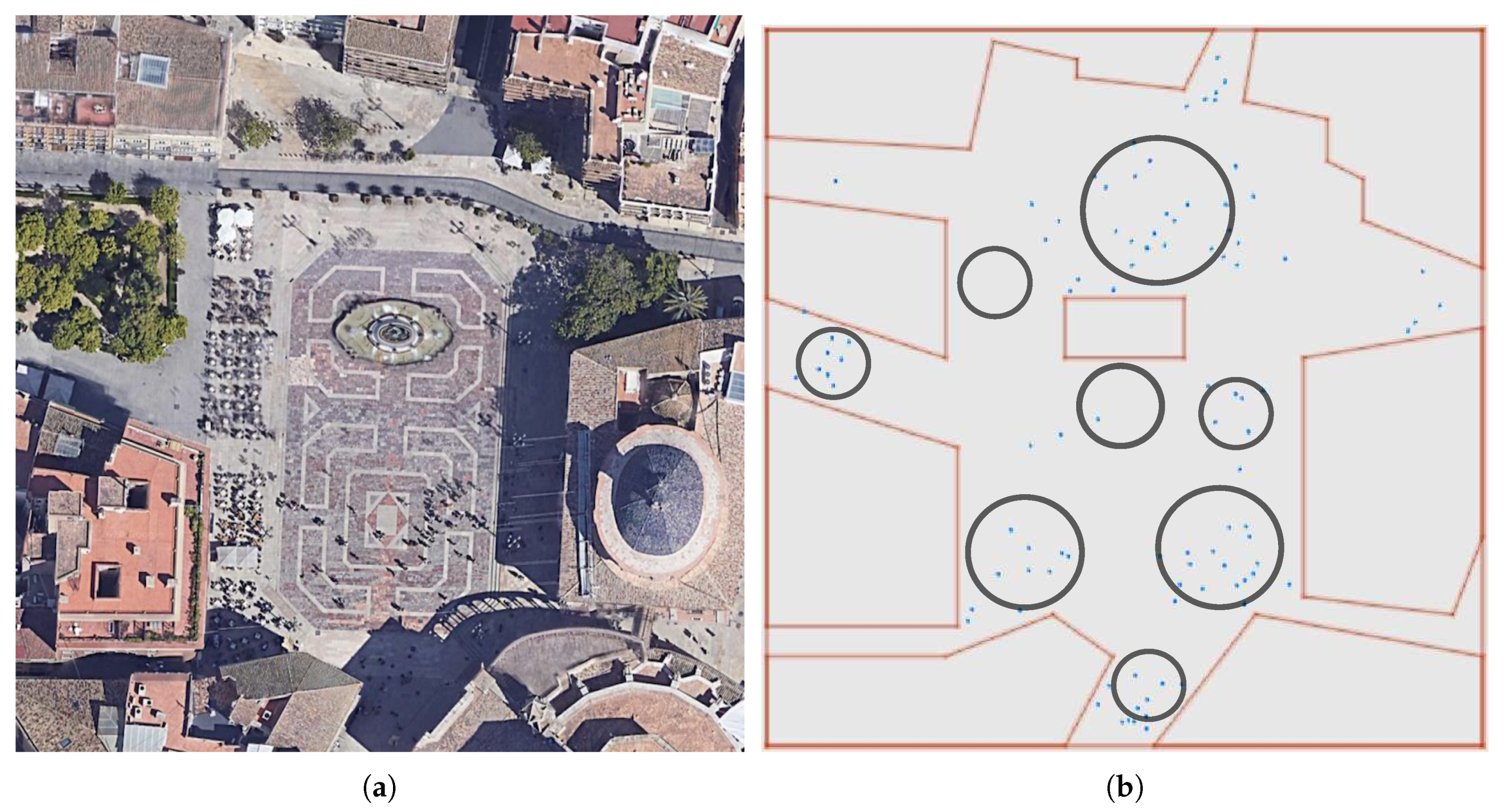
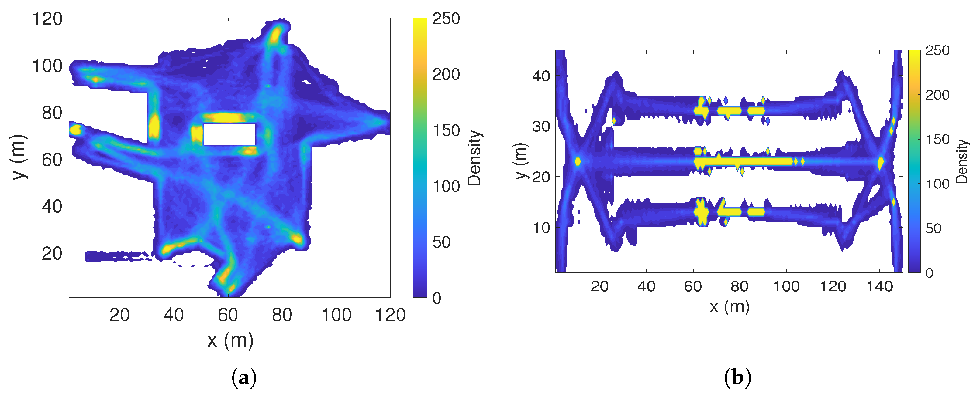
The first set of scenarios consist of 100 pedestrians moving freely on an open square area of 100 m × 100 m. We consider three synthetic models: Random WayPoint Model (RWP), Small World in Motion (SWIM), and RWPa, which is the RWP model with attraction points.

For generating the traces we used the BonnMotion tool [66]. BonnMotion is a free Java software which creates and analyses mobility scenarios and is most commonly used as a tool for evaluating OppNets and MANETs. It implements most of the synthetic models described in Section 3.1. Its main objective is to create mobility traces using mobility models.

The main parameters of the three synthetic scenarios are in

Table 1. Main parameters of the generated models.

Scenario	Nodes	Area	Other parameters
RWP	100	$100\mathrm{m}\times 100\mathrm{m}$	minSpeed = 0.5 m/s, maxSpeed = 1.5 m/s, maxPause = 60.0 s
SWIM	100	$100\mathrm{m}\times 100\mathrm{m}$	nodeRadius = 0.2 m, cellDistanceWeight = 0.5 m, nodeSpeedMultiplier = 1.5, waitingTimeExponent = 1.55, waitingTimeUpperBound = 50.0 s
RWPa	100	$100\mathrm{m}\times 100\mathrm{m}$	minSpeed = 0.5 m/s, maxSpeed = 1.5 m/s, maxPause = 60.0 s,          attractionPoints = $\{25,25,1.5,10,10,75,75,1.2,10,10,60,30,1.3,10,10\}$
Plaza	3050	$120\mathrm{m}\times 120\mathrm{m}$	$N_0=100,A_T=60s,P_R=50$
Station	1485	$150\mathrm{m}\times 50\mathrm{m}$	${\beta }_D=0.26,{\delta }_D=0.15,A_T=116,P_L=30.27,P_A=17.58,$$N_I=939,N_O=545$

. The first scenario, RWP, is a pure random scenario where pedestrians move according to the Random Waypoint model, with a random speed between 0.5 m/s and 1.5 m/s and a maximum pause of 60 s. SWIM is a more complex synthetic model, where each node is assigned a so-called home, which is a randomly and uniformly chosen point over the square area. Then, the node itself assigns to each possible destination a weight that grows with the popularity of the place and decreases with the distance from home. The parameters used for the generation are shown in Table 1.

Finally, the last scenario, RWPa, is an extension of the basic RWP model, where instead of choosing new destinations uniformly distributed from the simulation area, we can define attraction points. This way, we can set the locations where the pedestrians are more likely to move and stay (rather than moving randomly all over the defined area). Each attraction point is defined by five values: x and y coordinates, weight, and two standard deviations that are used to determine the nodes’ distances to the attraction point on both dimensions. Attraction points with higher weights will attract nodes with higher probabilities. In this scenario, we define three attraction points located in the following coordinates: (25,25), (75,75), and (60,30), with weights 1.5, 1.2, and 1.3. In all the points the two standard deviations used by the RWPa model to determine the nodes’ distance are set to 10.

4.2. Plaza Scenario

This scenario is an open square located in the city centre of Valencia, Spain. Locally known as “Plaza de la Virgen”, we will refer to it simply as Plaza. It is the typical tourist place that generally has a high degree of people renewal. The selected area has a dimension of $120\times 120$ m (you can see an aerial view in Figure 1a). From this real scenario, we define in PedSim an area with obstacles and open spaces where pedestrians can enter or exit as shown in Figure 1b.

The general process followed to generate the PedSim scenarios (the Plaza and Station scenarios) is the following: first, a text file (script) is created defining each the scenario. This script includes the main parameters, such as the speed of pedestrians, the points of interest through which they must pass, fixed obstacles, or walls. It is also necessary to define the time when every pedestrian enters or leaves the area. Second, this script is executed using PedSim in order to simulate the scenario. When the simulation ends, PedSim generates a trace file with the movement of all the pedestrians (time and location) with a resolution of 1 s.

Regarding the Plaza scenario, the pedestrian’s movement was generated considering that the plaza has an average number of 100 pedestrians, where 50 pedestrians are replaced every minute. The duration of the simulation is 1 h, so the final number of pedestrians that have passed through the plaza is 3050 (that is, $100+50\times 59$, the 100 initial pedestrians plus the 50 ones replaced every minute for the remaining 59 min.). Specifically, the renovation and movement of pedestrians were implemented as follows: the Plaza scenario has seven entry and exit accesses, and pedestrians are randomly placed at any of these entrances. The movement of pedestrians within the square follows the model of social force, as implemented by PedSim. These nodes are randomly assigned a displacement speed in the range of 0.3–1.5 m/s, moving between the main points of interest, delimited by the circles as shown in the Figure 1b. These points of interest are defined as the locations where pedestrians go and stay for a while, and which in this case represent monuments, restaurants, and terraces in the plaza. Regarding the renewal of pedestrians, in each renewal interval, a given number of nodes are randomly selected among the pedestrians that are inside the square. These nodes are notified to leave the plaza using one of the existing exits, and then 50 new nodes are created and placed randomly at one of the entrances to the plaza and move across the stage.

We also considered the social distancing into the mobility pattern generated by the PedSim simulator. One of the main recommendations for reducing the spread of the SARS-CoV-2 is keeping a safe space between oneself and other people. This increased physical distance has been considered in our model through the social force model used in the PedSim simulator. Particularly, in the simulator, two forces can be defined: the social force and the obstacle force. Higher values of these forces imply that the simulator tries to avoid close contact between pedestrians (or the obstacles). After several experiments, we set this social force to 7 (it can range from 0 to 10), in order to reduce, whenever it is possible, the close contacts (less than 2 m).

For parametrising this scenario, we have defined a set of parameters that are shown in Table 1, where $N_0$ is the initial number of pedestrians, $A_T$ is the average time between pedestrians renewals in seconds, and $P_R$ is the number of people that enter or exit at each renewal. This way, it would be easy to generate a new trace with other parameters.

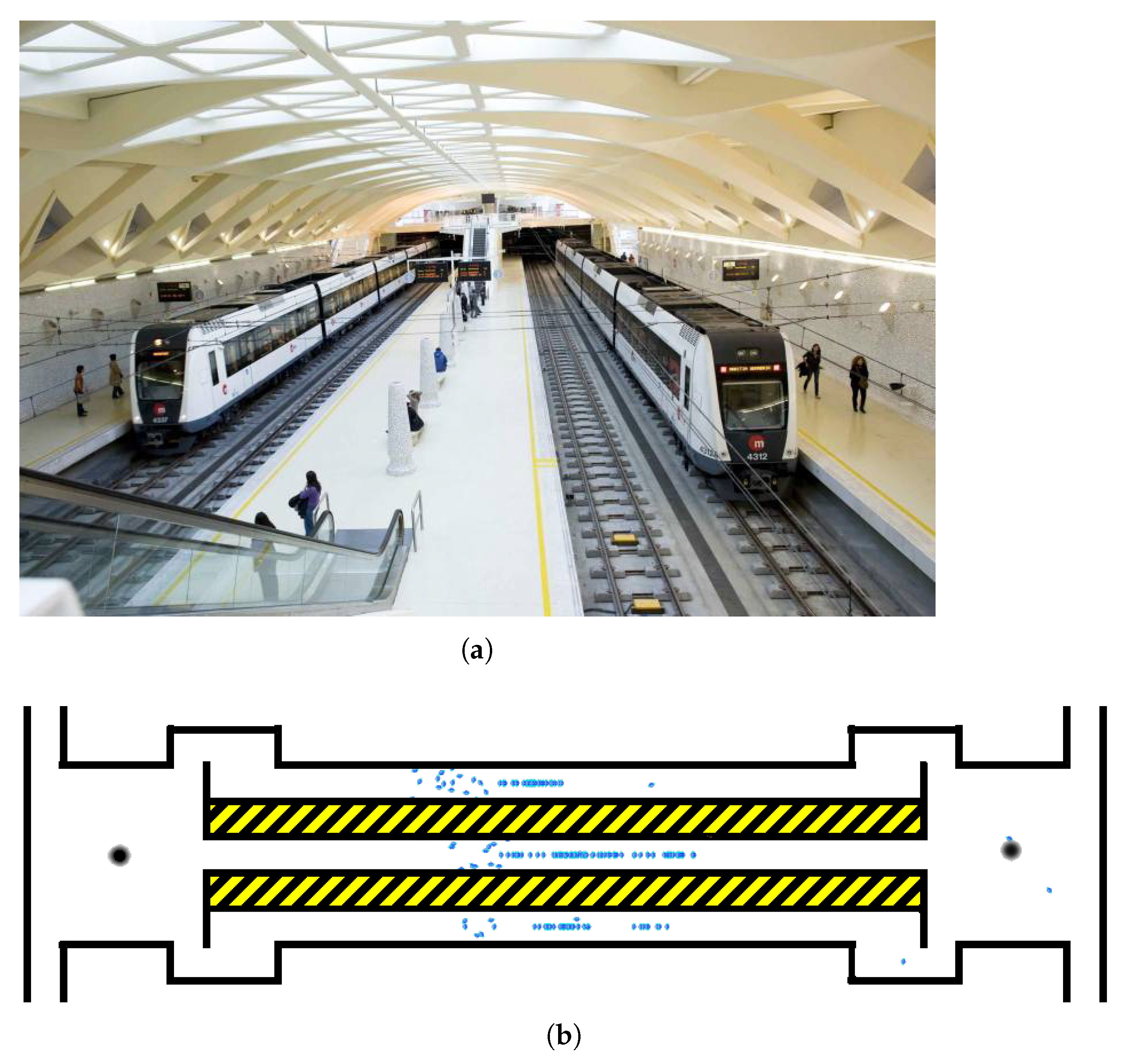
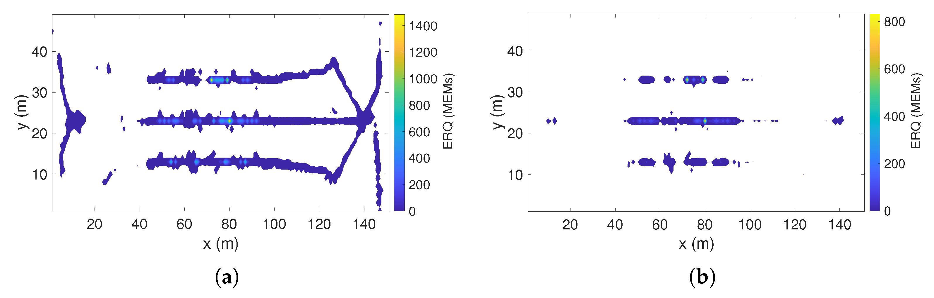
4.3. Station Scenario

Finally, this scenario is a closed space, a subway station, also located in the city of Valencia and locally known as “Alameda Station” (we will refer to it simply as the Station). This scenario represents a typical example of a crowded place, with different degrees of renewal and flows of people. This station has four tracks and three platforms: two side platforms and a central one, with an area of approximately 150 m$\times 50$ m. The platforms are accessible by stairs that can be reached through the four entrance doors located at each corner of the station, as can be seen in Figure 2. Four metro lines pass through this station, with an average interval between 5 min and 10 min.

To recreate the scenario, we took real measurements on 17 December 2020, from 8:00 a.m. to 9:00 a.m., by observing in-situ people arriving or leaving the station at different times of the day. Particularly, we measured the arrival time of the trains, the number of people who entered or left those trains, and the people who arrived from the four entrance doors. Based on these values, which are still valid for the current pandemic status, we simulated the subway station, considering as in the Plaza scenario, the social distancing of the current pandemic times.

In order to parametrise this scenario we have defined several metrics: the average rate of arrival ${\beta }_D$ and departure ${\delta }_D$ of the station using the entrance gates, the average time between trains $A_T$, and the average number of people arriving $P_A$ and leaving $P_L$ on each train. Using these values, we can obtain the whole number of people who have entered or left the station through the entrance doors ($N_I={\beta }_D·3600$ and $N_O={\delta }_D·3600$), as well as the number of people who have been at the station: $N=N_I+N_O$. The main parameters of the Station scenario are shown in Table 1.

Regarding PedSim, the scenario generation and pedestrian’s movement were implemented taking into account the previous values and the following aspects.

• People entering the Station. People enter the station through the doors of the main entrances. Specifically, for each of the four entrances, new pedestrians are generated according to a Poisson process with rate ${\beta }_D/4$, entering the station and passing through the turnstiles located at the two ends of the station. Then, each pedestrian is randomly directed with equal probability to one of the four platforms.
• Arrival of trains. The arrival times of the train are generated with the values obtained from the measurements. When a train arrives, pedestrians wait on the corresponding platform, get on the train, and disappear from the PadSim simulation. At the same time, pedestrians get off the train and enter the platform. From this platform, and for each pedestrian, a station exit door is randomly selected. Then, the pedestrians go directly to the selected gate and leave the station.
• Pedestrian’s movement: As in the Plaza scenarios, the movement of pedestrians follows the social force model with an average speed in the range of 0.3–1.5 m/s.

5. Evaluation of the Scenarios

The performance of Opportunistic Networks is based on the opportunity of contacts between mobile devices. Likewise, the spread of infections also depends on the physical contacts between humans. Therefore, in both cases, it is important to characterise individuals’ mobility. In this section, we analyse the traces generated from the different scenarios described in Section 4 considering both temporal and spatial aspects.

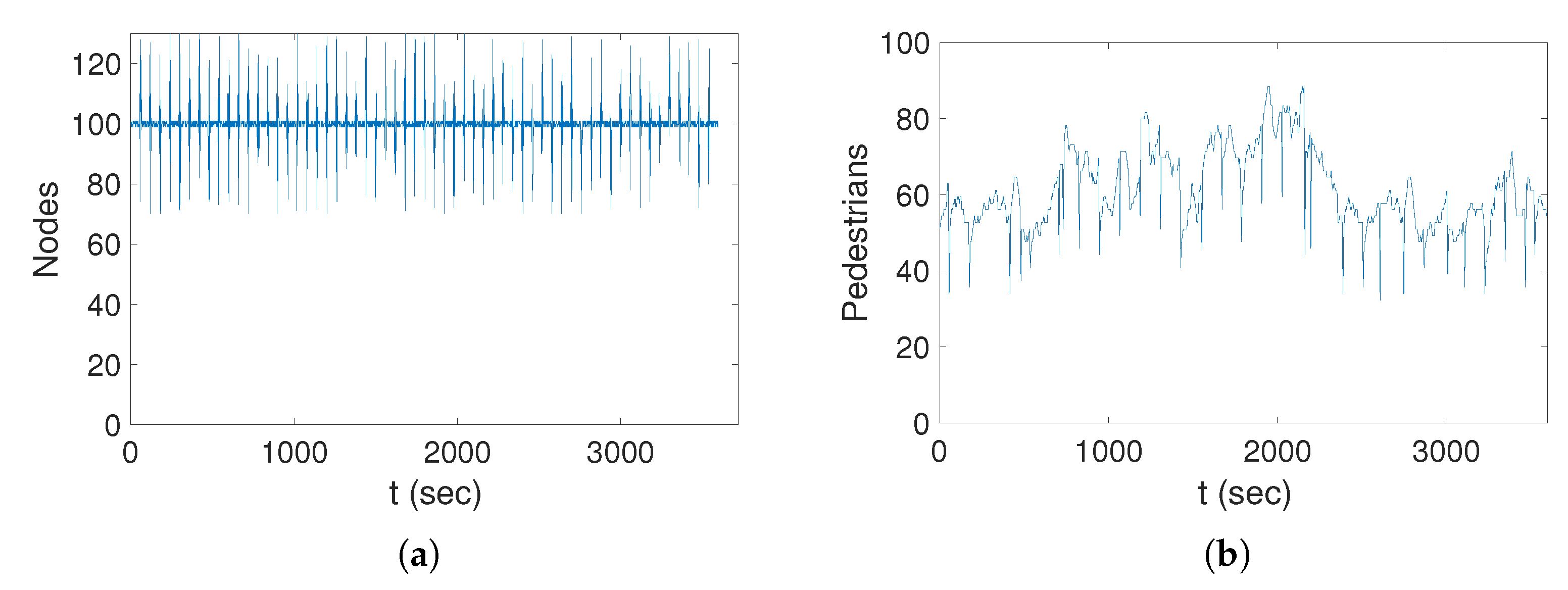
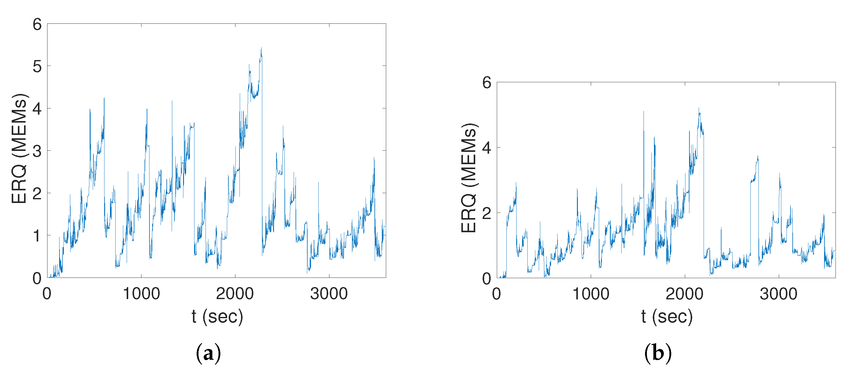
5.1. Temporal Evolution

In this subsection, we evaluate the number of individuals in the different scenarios depending on time. For the synthetic scenarios, the number of individuals is constant along time, so no further study is necessary. So, we focus our study on the Plaza and Station scenarios.

Figure 3 shows the number of nodes depending on time for the Plaza and Station scenarios. In the Plaza scenario (Figure 3a), we can see a periodical variation on the number of individuals, which corresponds to the every minute renewal of pedestrians in the Plaza. As expected, the average number of nodes is 100. Figure 3b shows the results for the Station scenario. We can see the variation in the number of individuals, which mainly depends on the arrival of the trains. The pattern is not completely periodical, since it depends on the real measured arrival times of the trains. In this scenario, the average number of individuals is 65.54.

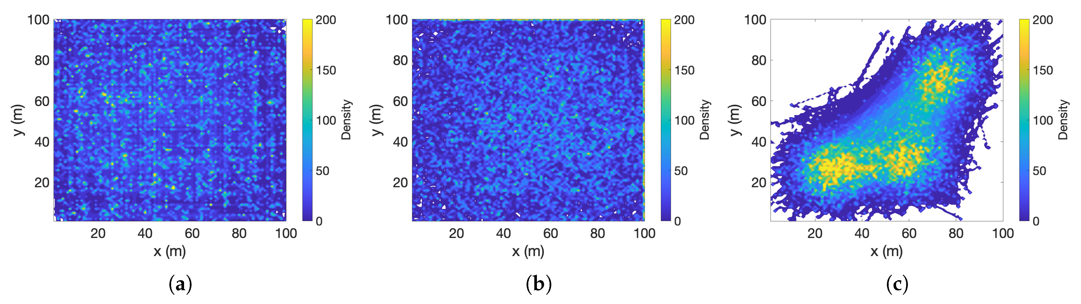
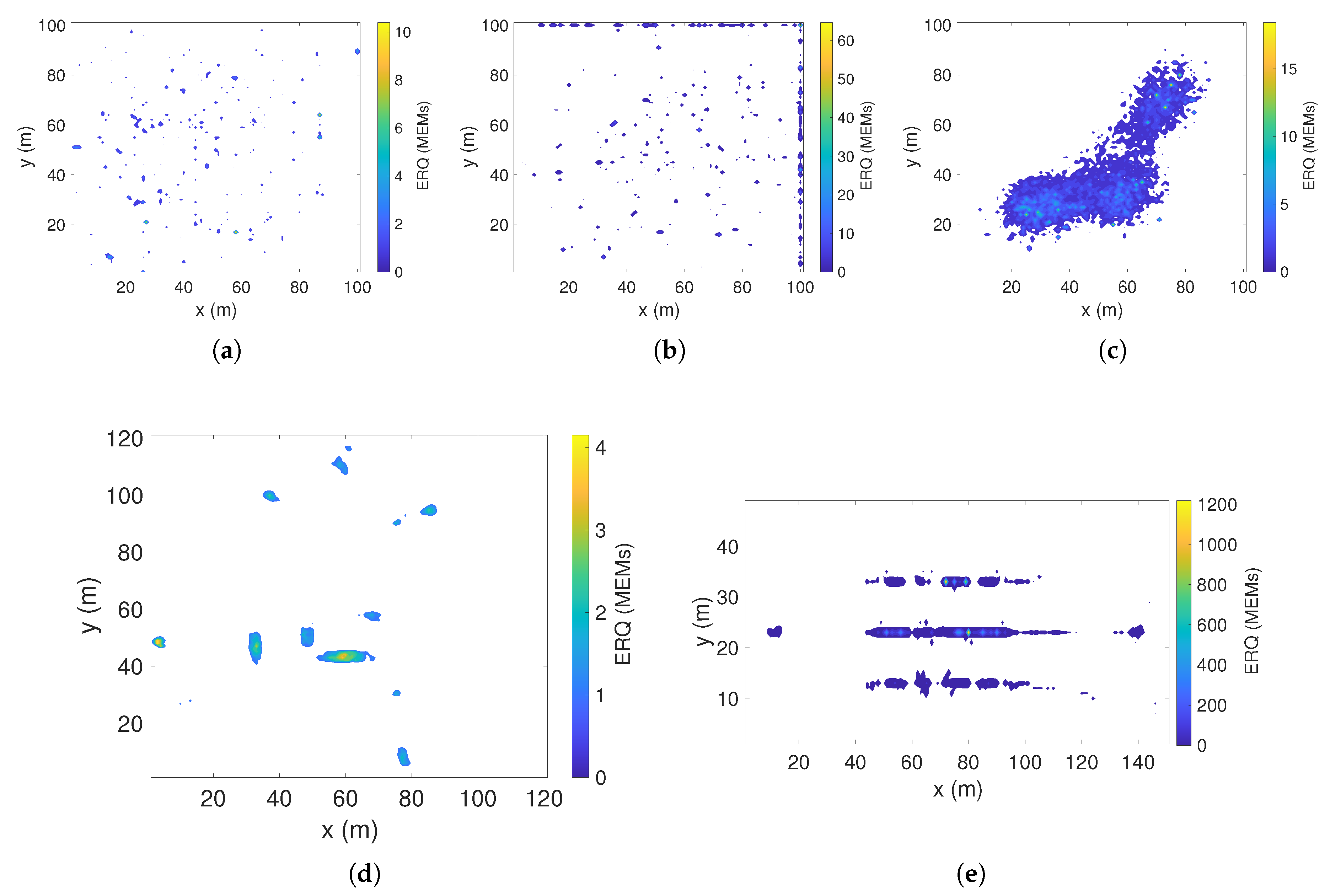
5.2. Spatial Distribution

Now we analyse the pedestrians’ movement in the different scenarios using density maps. For creating these density maps we used the previously generated mobility traces, considering a resolution of 1 m${}^2$ and 1 s. That is, the studied area is divided into cells of 1 m${}^2$, and for each cell, we obtained the accumulated number of seconds of all individuals that have been stayed in this cell. For example, a density value of 30 represents that individuals have stayed 30 s, which can be the result of a lot of different temporal and spatial combinations (for example, 2 individuals staying 15 s each one, or 30 individuals staying 1 s). This way, high-density cells represent places where more people stay.

Figure 4 shows the density maps for the synthetic scenarios. The results for RWP and SWIM are very similar, showing a completely random distribution of the density. For the RWPa scenario (Figure 4c), we can clearly see the effect of the attraction points, which are the areas with higher density and also the movement between these attraction points. Furthermore, the areas far away from these attraction points have not even been walked.

The density maps generated from the PedSim generated scenarios are shown in Figure 5. In the Plaza scenario (Figure 5a) we can see that the areas with more density correspond to the defined points of interest. We can also distinguish the main paths used for the pedestrians to enter and exit the plaza. For the Station scenario (Figure 5b), we can see that the higher densities are in the platforms, where the pedestrians stay and wait for the train. We can also observe the paths for entering and leaving the station, with some higher densities at the turnstiles where people wait to pass. Note that the turnstiles areas are at both sides of the figure, around the points (10,24) and (142,24).

Summing up, the results for the synthetic scenarios are very artificial, hardly representing any real scenario. Maybe the RWPa generated scenario could resemble some possible scenario, such as a shop. That is the main reason for using a pedestrian simulator, which generates a realistic scenario.

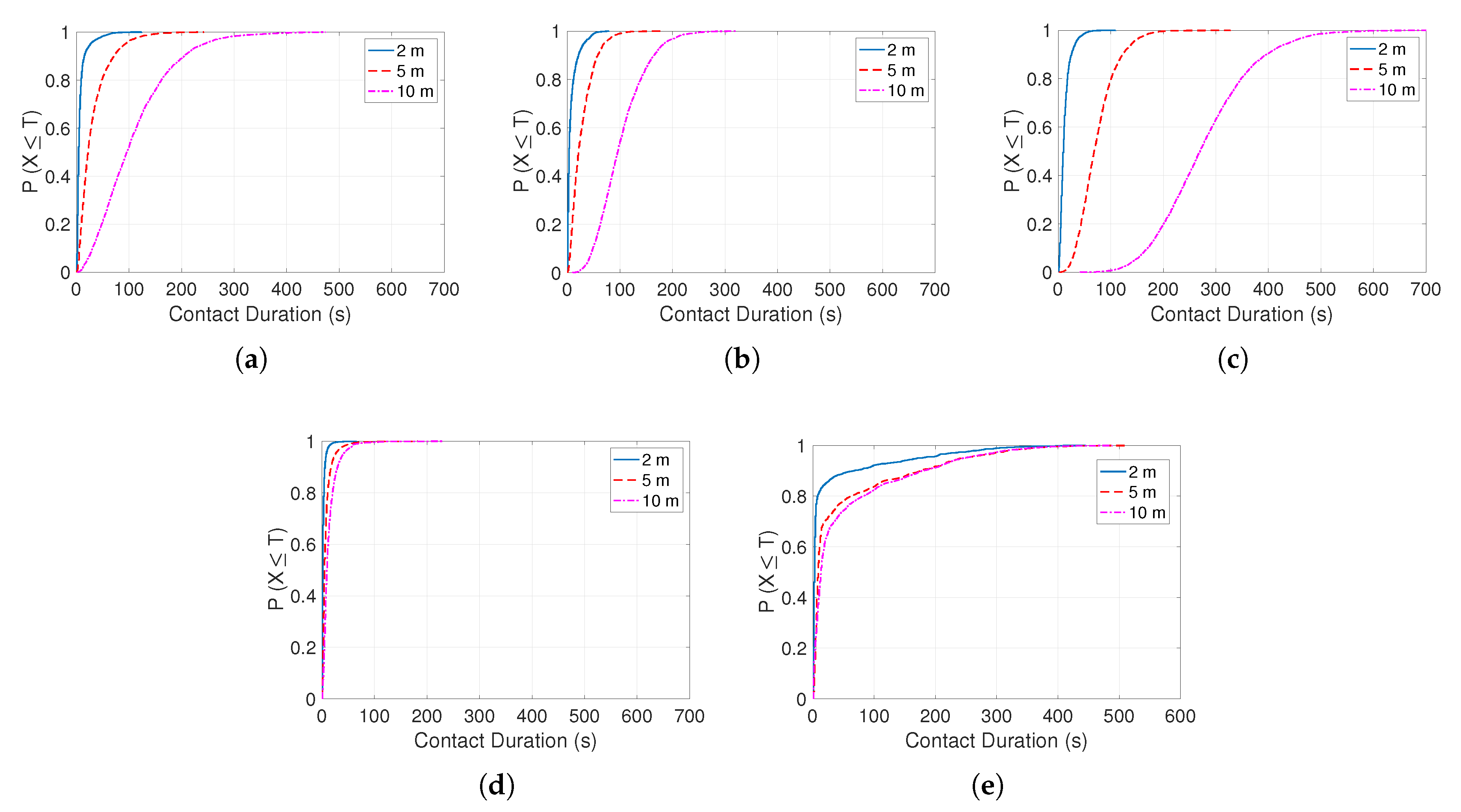
5.3. Physical Contacts Evaluation

The characterisation of the exposure risk to the virus will depend mainly on the distance and duration of a physical contact between two individuals. Note that physical contacts are all possible contacts which can be obtained from the traces of the different scenarios. The procedure to obtain these physical contacts is based on iterating over the traces and determining every second which pairs of nodes are within a determined distance range. This allows us to obtain the total number of contacts and their duration, in addition to the individuals’ location where the contact started.

Thus, in order to study these physical contacts, we consider the following different distances: 2, 5, 10 m. For each scenario and distance, we obtained all the possible contacts and their durations. Note that most pairs of individuals, particularly in the synthetic generated scenarios, can contact at different times and with different durations, so we also consider the accumulated duration of these contacts. For example, three different contacts between 2 individuals, with durations 2 s, 5 s, 1 s, results in an accumulated duration of 8 s. We use the accumulated duration since it reflects better the risk of exposure between a pair of individuals than considering only each contact separately. Thus, we obtain the following values:

• C: Number of Contacts. The whole number of generated contacts.
• P: Pairs Contacted. Number of different pairs of individuals that have contacted at least once.
• $P_D$: Distribution of the accumulated duration of the contacts between pairs.
• $E\left[D\right]$: Average accumulated duration obtained as the average of the previous distribution.

In

Table 2. The number of contacts, pair of individuals contacted and the accumulated average duration for the different scenarios and considering different distances.

	2 m			5 m			10 m
Scenario	C	P	$\mathit{E}\left[\mathit{D}\right]$	C	P	$\mathit{E}\left[\mathit{D}\right]$	C	P	$\mathit{E}\left[\mathit{D}\right]$
RWP	9660	2784	7.6	24,222	4340	31.61	47,104	4883	108.9
SWIM	12,368	3436	7.8	62,624	4934	27.7	213,222	4950	102.2
RWPa	31,778	4739	12.4	78,692	4948	73.9	143,874	4950	277.7
Plaza	44,714	14,108	2.8	90,514	33,990	8.2	154,930	60,375	13.9
Station	5941	2632	21.9	7212	3682	43.1	14,324	5961	49.2

we can see the number of contacts, pairs contacted and average contact time for the different scenarios and considering three distances. We also obtained the cumulative distribution function (CDF) of the accumulated contact duration $P(X\le T)$, as shown in Figure 6. Firstly, in Table 2 we can see the effect of social distancing on the PedSim generated mobility patterns: most of the contacts are greater than 2 m. Whereas in the Plaza scenario it was easy to keep this distance, the Station scenario evidences more difficulty for people keeping this distance, mainly when entering/exiting the train or passing through the turnstiles.

As expected, there is a clear dependence between distance and duration: the longer the considered distance of a contact, the longer the average contact duration. The longer contact times are obtained in the synthetic scenarios (RWP, SWIM, RWPa), which is due mainly to the no renewal of individuals. Additionally, for the RWPa scenario, we can see the effect of the attraction points, which generates a huge amount of contacts around these points. These results are confirmed with the CDFs (Figure 6). RWP and SWIM scenarios are quite similar, showing a high percentage of low duration contacts. Nevertheless, for the RWPa scenario, we can see that for a distance of 10 m, practically all contacts are in the range of [150, 400] s.

For the Plaza scenario, although the number of contacts is high, their duration is very short. This is due to the high renewal of individuals (note that every 60 s half of the individuals are renewed). Increasing the distance has little effect, as shown in the CDF in Figure 6d. Finally, for the Station scenario, we can find that the number of contacts is low although their duration is slightly longer. Nevertheless, note that this contact duration is also limited by the time people wait for the trains on the platforms. The CDF of this scenario (Figure 6e) exhibits a dichotomy in the duration of the contacts, since around 76% of the contacts have a duration less than 5 s, with a significant proportion of contacts between 5 and 300 s. This clearly reflects the two types of contacts that exist at the station: short-term contacts between people moving inside the station and long-term contacts for people waiting on the platforms. These duration patterns, as we will see in Section 7, will have a huge impact on the risk of infection.

6. Analysis of COVID-19 Transmission

The goal of this section is to analyse how the COVID-19 disease is transmitted and characterise the exposure to the virus, which will be used in the following section to evaluate the exposure risk for the different scenarios. The exposure risk is an important component of the reproduction number R.

The reproduction number R (or $R_0$ when it is measured without any intervention in disease transmission) is a simple and effective way to express how contagious an infectious disease is. R represents the average number of new infections an infected person can generate. Generally, the larger the value of R, the harder it is to control the epidemic. For example, first estimations of the $R_0$ value for the COVID-19 (that is, when no considering any measures) were between 2 and 3 [67,68], meaning that one infected person can transmit the disease to 2–3 persons. The reproduction number not only depends on the risk of exposure to the disease but also on other factors such as the duration of the individual’s infectiousness, the contact pattern, susceptibility of individuals, and population’s behaviour (that is, how population comply with the imposed measures, such as social distancing or lockdowns) [25,69].

Particularly, in this section, we focus our analysis on evaluating the transmission of the SARS-CoV-2 virus considering mainly the spatial, temporal, and environmental conditions of a given scenario. That is, the exposure risk to the virus when it enters the studied scenarios.

6.1. Background

In the case of SARS-CoV-2, it has been proven that its transmission is fundamentally airborne [9], mainly by droplets and aerosols. Viruses in droplets (larger than 100 $\mathsf{\mu }$m) typically fall to the ground in seconds within 2 m of the source. Because of their limited travel range, physical distancing reduces exposure to these droplets. Nevertheless, the SARS-CoV-2 virus is able to travel more than 2 m through aerosols (smaller than 100 $\mathsf{\mu }$m) emitted by infected people when breathing and can remain suspended in air for many seconds to hours. In both cases, droplets and aerosols, they are highly concentrated near an infected person, so they can infect people more easily in close proximity.

In order for the virus to establish and infect a new host, the receiving person must be exposed to this virus. The ease with which the virus can install itself in the receiving host depends on common and differentiated biological factors, as there are more genetically protected individuals than others. Not all exposed people are infected. However, the number of viral molecules that can land on the mucosa of another individual, and, therefore, the degree of success of the invasion is important and increases the chances that the virus will infect a new individual. Therefore, in this paper, we focus on evaluating only the exposure risk to the virus, without considering the receiver’s biological factors that can finally infect her/him, which can be defined as her/his immunity to the virus. Note that the final risk of transmission will be proportional to the exposure risk and inversely proportional to the immunity of the person.

To mathematically model the exposure risk ($ER$) we consider three main factors: the exposure time, the exposure intensity, and the quality of the medium. The goal is to have a simple and easy to understand expression to evaluate how the exposure risk depends on these factors. This way, we could easily communicate the main factors associated with the spread of the SARS-CoV-2 virus, including nonscientists such as policymakers and people in general. We are not pretending to obtain more realistic and complex expressions, like the ones developed in [28,29,30,31,32], which would require complex modelling and a lot of computational resources.

The exposure time (t) is the first important factor since it measures the time a person is exposed to the virus. That is, the longer the exposure time, the greater the number of viral molecules that reach the exposed person, and thus, the risk that some of them may prosper increases.

The second factor, the Exposure intensity ($I_x$), can be defined as the number of viral molecules reaching an individual per unit of time. Some authors use the concept of a quantum, as the dose of airborne droplet nuclei required to cause infection in 63% of susceptible persons) [29]. The exposure intensity factor depends on the intensity of the emitter, the proximity between individuals, and the quality of the medium between them. For example, a contagious individual, with a greater lung capacity or breathing rapidly, may emit a greater volume of aerosol, and, thus he/she emits with greater intensity or with a higher emission rate. This aerosol is rapidly diluted with distance and degrades with atmospheric agents. At a shorter distance, the viral concentration will be greater and the action of atmospheric agents will be less noticeable.

Finally, another important factor of the virus transmissibility is the quality of the medium ($Q_m$). A more aggressive medium (for the virus) where we can find UV radiation, a higher concentration of oxygen or chloride ions will reduce its effective transmission. On the contrary, a colder environment, air at rest, without direct sunlight will promote transmission of the virus. Virus transmission at low temperatures is more intensified by the ability of the air to maintain aerosols at lower temperatures. Furthermore, indoors the air is at rest, and the diffusion is uniform so the risk increases. Therefore, ventilation is a key element in reducing the risk of virus transmissibility.

The medium can be analysed in greater detail. As previously said, exposure intensity will be lower in open or ventilated premises compared to enclosed ones. This intensity can be reduced in closed premises through well-designed air recirculation systems. Nevertheless, low temperature allows the aerosol to remain in the environment for longer. For example, there have been many COVID-19 outbreaks in meat and cold cut processing plants. In such places, the indoor temperature may be below dew temperature and air conditioning recirculation systems can distribute potentially contaminated air to all rooms.

Summing up, the exposure risk ($ER$) will be proportional to the exposure time t and the exposure intensity $I_x$:

$$ER=K·t·I_x$$

(1)

where K is a constant for adjusting the model. For determining how the exposure intensity $I_x$ depends on the distance d, we employ a simple physical model of the dispersion of particles (in this case, the virus in aerosols). Concretely, we consider that diffusion decays with the squared distance from the emitter. Consequently, $I_x$ is proportional to the emitter intensity ($I_e$) and inversely proportional to the square of the distance (d) between the individuals:

$$I_x=Q_m\frac{I_e}{d^2}$$

(2)

where $Q_m$ is a factor which depends on the quality of the medium.

In our model, as we want to obtain a spatial and temporal evaluation of the exposure risk, we consider that all people in the scenario to evaluate are potentially infectious. Of course, the real risk will depend on the real number (or density) of contagious people in the scenario. Indeed, in a place with no contagious people, the real risk will be zero. The idea is that each contact can be risky (when you enter a place, you do not know if there are contagious people or not and who they are). Assuming also that the intensity of the emission is the same for all emitters, we can simplify the previous expression, considering $I_e$ to be one. This is the same approach that other authors make when considering the quanta emission rate to be constant [28]. Thus, combining Expression (1) with the simplified expression of $I_x$, we have:

$$ER=K·Q_m\frac{t}{d^2}$$

(3)

Thus, using this expression we can obtain the exposure risk to the COVID-19 infection. This risk, understood as the possibility that a person could be infected, depends on the quality of the medium and is directly proportional to the time and inversely proportional to the square of the distance that separates the person from the contagious individual.

Now, we will characterise the quality of the medium as the factor $Q_m$, based on the study of Jimenez et al. [31] about the physical conditions which impact the SARS-CoV-2 virus airborne transmission. When $Q_m=1$ the medium will be optimal for the virus transmissibility and corresponds to a medium in which the following circumstances concur: (i) Enclosed space (height less than 3 m); (ii) No ventilation; (iii) Low temperature (between 0 and 7 degrees Celsius), and (iv) Artificial lighting. On the contrary, in less advantageous scenarios (for the virus transmissibility), the $Q_m$ values will be lower than the unit, and thus, reducing the risk of contagion. A medium very hostile to transmission is characterised with the following conditions: (i) an open space; (ii) windy; (iii) high temperature, and (iv) solar lighting (due to the presence of UV rays that are destructive for the SARS-CoV-2 virus).

This low-quality medium, for example, could correspond to a beach in the summertime. However, although in these environments the value of $Q_m$ will be very low, the virus transmission may occur between close and long duration contacts. Therefore, we cannot make the quality factor null even in this case. It will only be null when there is a barrier that prevents transmission. Note that in this quality of the medium we do not consider physical barriers such as face-masks, screens, or plastic sheets.

Finally, in order to assign a value to $Q_m$, we consider that there are three major factors that determine the quality of the medium: the renewal of air, temperature, and solar radiation, each one with three levels of quality: good (1), moderate (2/3), and bad (1/3) (see

Table 3. Quality of the medium. Assignment of values. Good stands for good quality of virus transmission and it means no air renewal, low temperature, and no solar radiation.

Quality of the Medium	Good	Moderate	Bad
Air renewal	1	2/3	1/3
Temperature	1	2/3	1/3
Solar radiation	1	2/3	1/3
Value	1	2/3	1/3

). We do not consider if the space is open or closed since it clearly determines the other factors. The weight that each of these factors can have on the quality of the medium is currently an unknown. Roughly we can give them the same weight. Thus, the goal of Table 3 is to calculate the value of $Q_m$ depending on the characteristics of the scenario to evaluate. We keep it simple enough in order to be easy to apply in any scenario, although it could be possible to assign intermediate values (for example, if the air renewal quality is between good and moderate we can consider a value of 5/6).

We can use Table 3 to estimate the value of the quality of the medium ($Q_m$) in the Plaza and Station scenarios. The maximum value, as we have already seen, will be 1 and in the most unfavourable medium, it will drop to 1/3. For the Plaza scenario we consider a final value of $Q_m=1/3$, as it is an open space with high air renewal (1/3), high temperatures (1/3) and solar radiation (1/3). We are considering a sunny day (Valencia city has very good weather all year round). For the Station scenario, we consider a global moderate quality of the medium $Q_m=2/3$. It is a high-rise venue with open doors and air circulation inside so the air renewal is moderate (2/3). The temperature is similar to the previous scenario (1/3), and solar radiation is very low, so those are better conditions for virus transmission transmission (1). Averaging these factors, we have $Q_m=(1+1/3+2/3)/3=2/3$.

6.2. Exposure Risk Characterisation

Based on the previous studies, in this subsection, we propose two alternative methods to obtain the exposure risk. The first one is based on obtaining the risky contacts, that is, the contacts which can be susceptible to transmit the disease. The second method is based on Expression (3), which is a more generic expression of the exposure risk considering also the impact of the environment.

According to the European Centre for Disease Prevention and Control (ECDC) [70], a contact is classified with high-risk exposure if a person has had face-to-face contact with a COVID-19 case within 2 m for more than 15 min (900 s). The USA’s CDC (Centers for Disease Control and Prevention) [71] also has a similar definition: an individual who has had close contact (less than 6 feet $\approx 1.83$ m ) for 15 or more min. Following these strict criteria, no contact in the generated scenarios would be considered a high-risk exposure, since for 2 m the maximum contact duration is 500 s (less than 8 min), as can be seen in Figure 6.

Nevertheless, recent studies [9,72] have shown that all exposure time counts and even the CDC has revised its guidance, acknowledging that even brief contacts can lead to transmission. So, a more useful approach is to measure the number of minutes exposed to risky contacts. This is the last method used by the smartphone-based contact tracing apps using the Application Program Interface (API) jointly developed by Apple and Google. Apple has defined an Exposure Risk Value (ERV) to allow health authorities to define when to alert a user that they may have been exposed to someone diagnosed with COVID-19 which is measured in Meaningful Exposure Minutes (MEMs) units [73]. Although ERV offers flexibility in calculating this value by setting weights and values related to bluetooth attenuations, the infectiousness of the affected individual and diagnosis report type, in this paper we will obtain only the minutes exposed to a contact. For example, an ERV of 10 MEMs reflects that an individual has been exposed to risk contacts for an accumulated time of 10 min.

Nevertheless, the ERV only takes into account the (discretised) distance and time of the contacts, omitting the impact of the environment. Thus, based on the previous study of Section 6.1 we propose the following expression, Exposure Risk with Quality (ERQ), which is not only based on the (continuous) distance and time between individuals but also on the quality of the medium:

$$ERQ=K·Q_m\frac{t}{max{(d,0.3)}^2}$$

(4)

This expression is a slight adaption of Expression (3). The risk is inversely proportional to the square of the distance, so for long distances, the exposure risk will be practically negligible. On the contrary, for very close encounters the risk will increase exponentially, up to 0.3 m, which is the minimum interpersonal distance [74]. Note that this limit also avoids a singularity at $d=0$.

In order to normalise this expression, we use the same units (MEMs) than in the previous ERV expression. For obtaining the value of K in expression, we consider that one minute of MEMs is equivalent to a contact with a duration of one minute and within a distance of one metre (the average distance used in the ERV), considering also an average quality of the medium ($Q_m=0.5$). Therefore, if t is expressed in minutes and d in metres, and working out the value of K in Expression (4) we obtain a value of 1/30 m${}^2$.

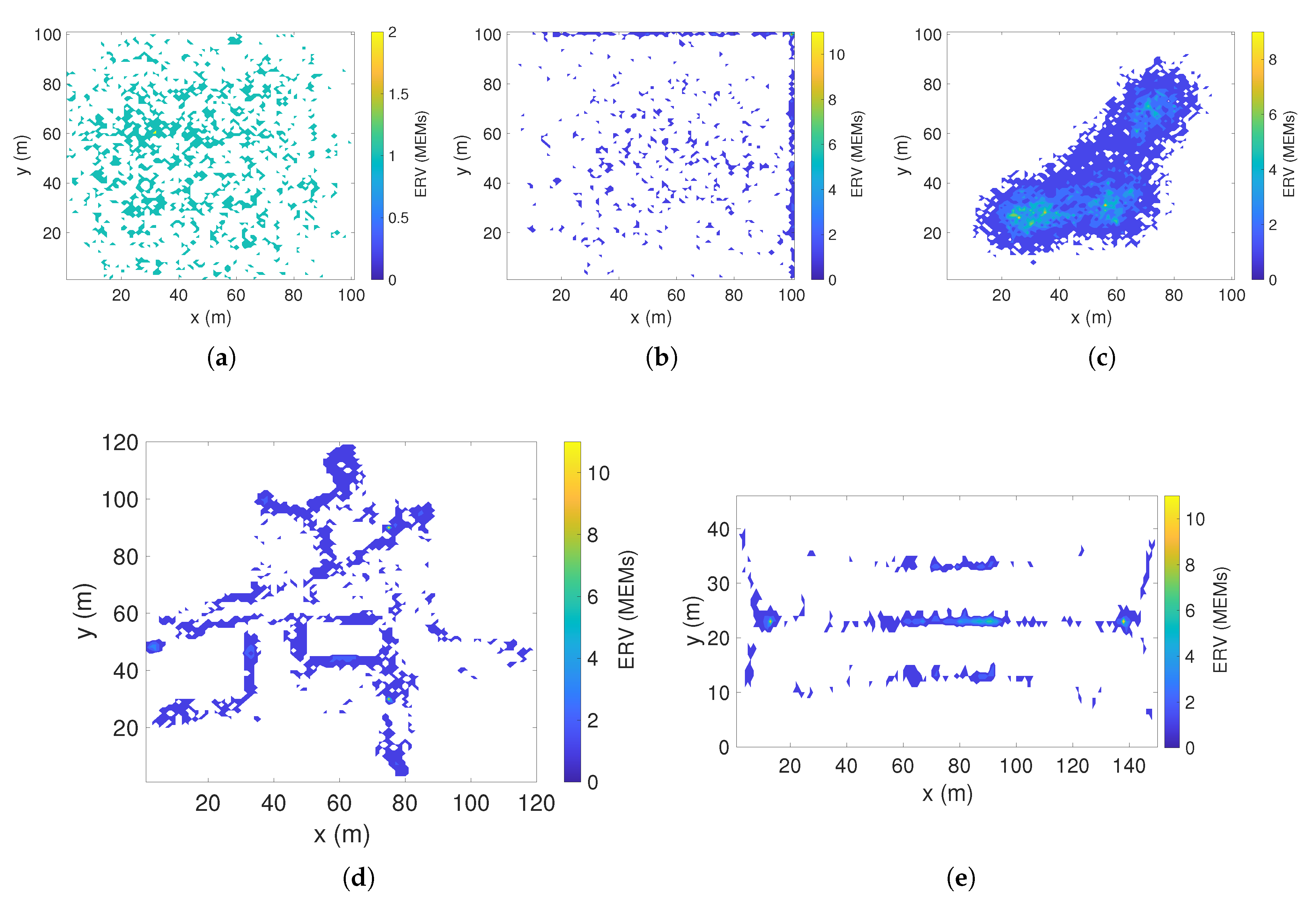
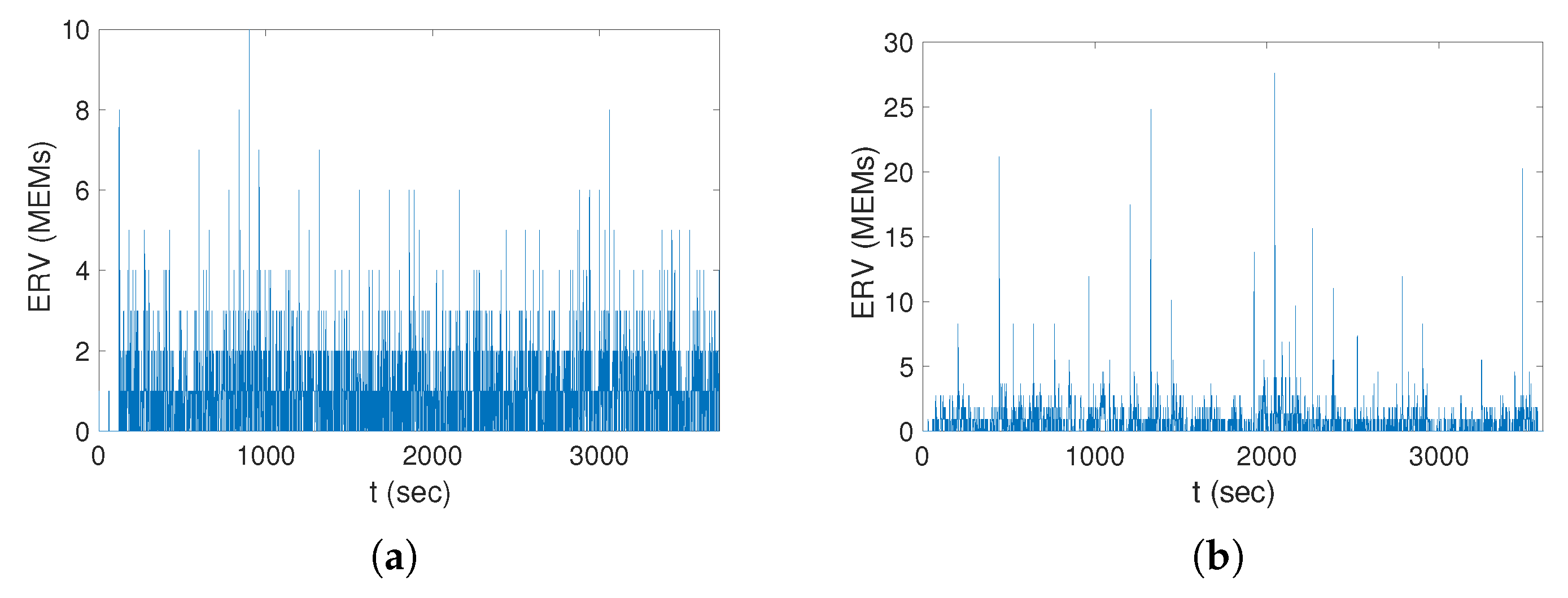
7. Evaluation of the Infection Risk

In this section, we evaluate the exposure risk in the generated scenarios. The idea is to determine the areas where there is more risk of infection and the temporal evolution of the exposition. As expected, some of these areas coincide with the areas with higher density studied in Section 5, but they provide a better delimitation of the risky spots.

7.1. ERV Evaluation

We first analyse the results obtained using the Exposure Risk Value (ERV) measured in Meaningful Exposure Minutes (MEMs) units, as described in Section 6.2. In this evaluation, as in Section 5.2, the evaluated area is divided into cells of 1 m${}^2$, and for each cell, we obtain the accumulated ERV of all people contacts initiated in this cell.

In detail, the method for obtaining the contacts and the cell’s ERV is the following: using the position traces generated from the different scenarios, we determine every second which pairs of nodes are within the 2 m range. If the duration of the contact is greater than 1 min, this duration is added to the cells where the contact started. This means that, since every contact involves two individuals, we add the associate ERV of these contact to two cells, which corresponds to the cell where each individual was when the contact started. This way, we can obtain a measure of the risk of each cell measured in MEMs.

Figure 7 shows the ERV heat maps for the five scenarios. Starting with the RWP and SWIM scenarios, we can see that there are small risky spots randomly distributed throughout the area, although in the SWIM scenario there are more risks at the edges. In the RWAa, as expected, the risky areas are around the attraction points, due to the high number of contact generated near to these points. For the Plaza scenario, we can see that the risky areas are also around the attraction points and along the entry and exit paths. Finally, for the Station scenario, the risky areas are in the centre of the platforms and near the turnstiles, where the contact have longer durations.

Now, we study the temporal evolution of the exposure risk. This risk is also measured using MEMs and represents the current ERV depending on time, that is, the aggregated minutes of all risky contacts which are active at the given time. For the synthetic scenarios, the evolution is quite constant, so we do not show here the results. More interesting are the results for the PedSim generated scenarios shown in Figure 8. For the Plaza scenario, we can see the variability of the risk depending on the periodical renewal of the people. In addition, in the Station scenario, we can see the impact of the trains arrivals. The ERV peaks coincide with the arrivals of the trains.

7.2. ERQ Evaluation

The previous experiments only considered the impact of distance and time. Nevertheless, it is essential to evaluate the impact of the environment on the risk. For example, there is strong evidence that indoor airborne transmission of the COVID-19 is much higher than in outdoor spaces, particularly in crowded environments such as a station.

Thus, we repeated the previous experiments using Expression (4) for evaluating the spatial and temporal risk exposure. Unlike the previous ERV evaluation, we do not consider explicitly contacts between pairs. Instead, we obtain the risk of each pair of individuals that are in the scenario. The procedure is the following: every second and for each pair individuals in the scenario, we calculate their ERQ, considering an elapsed time of $t=1$ s. This ERQ, measured in equivalent MEMs, is added to the cells where the individuals were in that moment, in order to obtain a measure of the exposure risk in each cell.

Regarding the quality of the medium ($Qm$), since the three synthetic scenarios do not correspond to a real scenario, we set a value of $Q_m=0.5$ (we cannot use Table 3. Regarding the other two real scenarios, as detailed in Section 6, we consider $Q_m=1/3$ for the Plaza scenario, which corresponds to an open space with high solar radiation, and $Q_m=2/3$ for the Station scenario, which corresponds to an indoor space with high ceilings and with poor ventilation.

The results of the spatial exposure risk are shown in Figure 9. For the synthetic scenarios, we can see that the patterns are similar to the results obtained for the ERV. Nevertheless, the obtained MEMs are in general greater than using ERV, showing a higher exposure risk. This is mainly due to the way the exposure risk of a cell is obtained: in ERQ, each second of exposure is added up while for ERV only contacts with duration longer than 1 minute is considered.

For the Plaza scenario (Figure 9d) we can see, as expected being an open space, that the exposure risk has been reduced considerably when compared to the previous ERV results. Only in some small spots, there is a small exposure risk, which corresponds to the locations where people stay. On the contrary, the Station scenario (Figure 9b displays a high exposure risk, particularly on the centre of the platforms and turnstiles, which are in general much higher than in the ERV evaluation. These results do not only depend on the value of $Q_m$ but also on the number of contacts and their short proximity, not accounted for when using the previous ERV model.

As in the ERV evaluation, we study the temporal evolution of the risk, obtaining for each second the aggregated equivalent MEMs between all pair of individuals in the scenario. We only show in Figure 10 the results for the Plaza and Station scenarios. Firstly, we can see that the ERQ is now a continuous plot (compared to the discrete plot of Figure 8). For the Plaza scenario, we can see that the exposition risk is very low. In the Station scenario, we can clearly see a higher exposure risk and observe graphically how this risk increases when people crowd the platform waiting for the trains.

Finally, we evaluate the impact of social distancing on the exposure risk. Along with the use of face masks, social distancing has been seen as one of the most effective measures that people can take. So, it is important to evaluate its impact to reduce the COVID-19 disease. As detailed in Section 4, the PedSim simulator can be parametrised in order to generate mobility traces with different social distances. All previous experiments were done using a social force of 7, which was adjusted to avoid close contacts (less than 2 m). We centre our evaluation on the spatial risk of the Station scenario using ERQ (that is, as shown in Figure 10b). We repeated the same experiment considering two different social forces. If the social force is set to a low value (2), the simulator will reduce the distance between pedestrians. In contrast, if this value is set very high (9), it will increase the physical distance between pedestrians (whenever it is possible). Note that a very low value (0–1) is unreal, and actually, it will simulate collisions between pedestrians.

The results are shown in Figure 11, and we compare them with the previous results of Figure 10b). On the one hand, we can see in Figure 11a that, when no social distance measures are taken, the exposure risk significantly increases throughout all the station and not only on the expected hot spots (platforms and turnstiles). On the other hand, if this distance is increased, we can clearly see in Figure 11b that the exposure risk is greatly reduced, although there are spots where the distance cannot be reduced, so the risk is still there. This experiment evidences the flexibility of our proposed model since it can study how different human mobility patterns can affect the spreading of the COVID-19 disease.

Summing up, the previous experiments show that using a proper expression of exposure risk we can obtain the spots where the risk is high, and also, compare the results of the different scenarios (that is, outdoor vs. indoor). Particularly, in the scenarios evaluated, the Plaza outdoor scenario exhibits a very reduced risk exposure compared to the Station indoor scenario.

Based on these results, health authorities could make effective risk management plans to force pedestrians to avoid these risky spots with the final objective of minimising the risk of transmission. For example, the map can be used in the station scenario to mark with arrows and lines enter and exit routes, places to stay, etc. Furthermore, this plan could be modelled again in the pedestrian simulator (for example, defining the safe routes) in order to test if the proposed plan is correct or not (that is, no hot spots are generated). This can be an iterative process until a good plan is obtained. This is similar to the primary use of pedestrian simulators, in which architects and civil engineers assess the impact of different levels of pedestrian demand, and test and validate emergency evacuation plans. Finally, a different approach would be to increase ventilation in the place or even using an autonomous robot to disinfect the risky spots continuously.

8. Conclusions

In this paper, we have studied how human mobility models can be used to evaluate the risk of infectious diseases, particularly for COVID-19. Mobility models have been used to evaluate the diffusion of messages on mobile computer networks and opportunistic networks. We evaluated two different sets of mobility models: pure synthetic models and models based on mobility simulators. For the latter, we created two realistic urban scenarios: a plaza and a subway station. Particularly interesting are the scenarios generated with the mobility simulator.

For evaluating the exposure risk, we used two models. The first one is based on the method used by smartphone-based contact tracing applications, which only considers time and distance. For considering the environment, we introduced a new expression where the quality of the medium is determined by the type of scenario.

The results show that pure synthetic models cannot offer realistic human mobility patterns and therefore the risk maps obtained using these models are not useful. On the other side, using the scenarios generated with the pedestrian simulator we can obtain heat maps of the exposure risk where we can easily discern the risky spots. Furthermore, using the second risk model, we can see that outdoor scenarios, such as the plaza, exhibit a very low-risk exposure when compared to indoor scenarios, such as the Station.

Summing up, the proposed model is a novel and promising approach to evaluate the exposure risk of any scenario, particularly considering people mobility, which is one of the key factors in the spreading of infectious diseases. The combination of human mobility scenarios generated using a pedestrian simulator with the evaluation of risk exposure would allow authorities to assess the risk of any crowded places and then take measures, such as risk management plans, so the transmission of the COVID-19 can be reduced. As future work, we plan to improve our model using more complex diffusion models or even considering new risk factors when new details affecting the spread of the SARS-CoV-2 are discovered.

References

1. Eames, K.; Keeling, M. Contact Tracing and Disease Control. Proc. Biol. Sci. R. Soc. 2004, 270, 2565–2571. [Google Scholar] [CrossRef] [Green Version]
2. Salathé, M. Digital epidemiology: What is it, and where is it going? Life Sci. Soc. Policy 2018, 14, 1. [Google Scholar] [CrossRef] [PubMed]
3. Singapore Government. Tracetogether. Available online: https://www.tracetogether.gov.sg (accessed on 15 April 2020).
4. PePP-PT e.V. i.Gr. Pan-European Privacy-Preserving Proximity Tracing (PEPP-PT). Available online: https://www.pepp-pt.org (accessed on 15 September 2020).
5. Hernández-Orallo, E.; Manzoni, P.; Calafate, C.T.; Cano, J. Evaluating How Smartphone Contact Tracing Technology Can Reduce the Spread of Infectious Diseases: The Case of COVID-19. IEEE Access 2020, 8, 99083–99097. [Google Scholar] [CrossRef]
6. Hernández-Orallo, E.; Manzoni, P.; Calafate, C.T.; Cano, J. Evaluating the Effectiveness of COVID-19 Bluetooth-Based Smartphone Contact Tracing Applications. Appl. Sci. 2020, 10, 7113. [Google Scholar] [CrossRef]
7. Zhang, X.; Neglia, G.; Kurose, J.; Towsley, D. Performance modeling of epidemic routing. Comput. Netw. 2007, 51, 2867–2891. [Google Scholar] [CrossRef]
8. Helgason, Ó.; Kouyoumdjieva, S.T.; Karlsson, G. Opportunistic Communication and Human Mobility. IEEE Trans. Mob. Comput. 2014, 13, 1597–1610. [Google Scholar] [CrossRef]
9. Prather, K.A.; Marr, L.C.; Schooley, R.T.; McDiarmid, M.A.; Wilson, M.E.; Milton, D.K. Airborne transmission of SARS-CoV-2. Science 2020, 370, 303–304. [Google Scholar]
10. Nishiura, H.; Oshitani, H.; Kobayashi, T.; Saito, T.; Sunagawa, T.; Matsui, T.; Wakita, T.; Suzuki, M. Closed environments facilitate secondary transmission of coronavirus disease 2019 (COVID-19). medRxiv 2020. [Google Scholar] [CrossRef] [Green Version]
11. Vukadinović, V.; Helgason, Ó.R.; Karlsson, G. An analytical model for pedestrian content distribution in a grid of streets. Math. Comput. Model. 2013, 57, 2933–2944. [Google Scholar] [CrossRef]
12. Chancay-García, L.; Hernández-Orallo, E.; Manzoni, P.; Calafate, C.T.; Cano, J. Evaluating and Enhancing Information Dissemination in Urban Areas of Interest Using Opportunistic Networks. IEEE Access 2018, 6, 32514–32531. [Google Scholar] [CrossRef]
13. Christaki, E. New technologies in predicting, preventing and controlling emerging infectious diseases. Virulence 2015, 6, 558–565. [Google Scholar] [CrossRef] [Green Version]
14. Grossglauser, M.; Tse, D.N.C. Mobility increases the capacity of ad hoc wireless networks. IEEE/ACM Trans. Netw. 2002, 10, 477–486. [Google Scholar] [CrossRef]
15. Chaintreau, A.; Hui, P.; Crowcroft, J.; Diot, C.; Gass, R.; Scott, J. Impact of Human Mobility on Opportunistic Forwarding Algorithms. IEEE Trans. Mob. Comput. 2007, 6, 606–620. [Google Scholar] [CrossRef]
16. Garg, K.; Giordano, S.; Förster, A. A Study to Understand the Impact of Node Density on Data Dissemination Time in Opportunistic Networks. In Proceedings of the 2nd ACM Workshop on High Performance Mobile Opportunistic Systems HP-MOSys ’13, Barcelona, Spain, 3–8 November 2013; ACM: New York, NY, USA, 2013; pp. 9–16. [Google Scholar]
17. Lin, Y.; Wang, X.; Zhang, L.; Li, P.; Zhang, D.; Liu, S. The impact of node velocity diversity on mobile opportunistic network performance. J. Netw. Comput. Appl. 2015, 55, 47–58. [Google Scholar] [CrossRef]
18. Su, J.; Chin, A.; Popivanova, A.; Goel, A.; de Lara, E. User mobility for opportunistic ad-hoc networking. In Proceedings of the Mobile Computing Systems and Applications, Windermere, Cumbria, UK, 3 December 2004; pp. 41–50. [Google Scholar]
19. Feng, Z.; Chin, K.W. A Unified Study of Epidemic Routing Protocols and Their Enhancements. In Proceedings of the 2012 IEEE 26th International Parallel and Distributed Processing Symposium Workshops & PhD Forum, Shanghai, China, 21–25 May 2012; IEEE Computer Society: Washington, DC, USA, 2012; pp. 1484–1493. [Google Scholar]
20. Moreira, W.; Mendes, P. Impact of human behavior on social opportunistic forwarding. Ad Hoc Netw. 2015, 25 Pt B, 293–302. [Google Scholar] [CrossRef] [Green Version]
21. Zhang, Y.; Zhao, J. Social Network Analysis on Data Diffusion in Delay Tolerant Networks. In Proceedings of the Tenth ACM International Symposium on Mobile Ad Hoc Networking and Computing (Mobihoc’09), New Orleans, LA, USA, 18–21 May 2009; ACM: New York, NY, USA, 2009; pp. 345–346. [Google Scholar]
22. Herrera-Tapia, J.; Förster, A.; Hernández-Orallo, E.; Udugama, A.; Tomas, A.; Manzoni, P. Mobility as the Main Enabler of Opportunistic Data Dissemination in Urban Scenarios; Springer International Publishing: Cham, Switzerland, 2017; pp. 107–120. [Google Scholar]
23. Bettstetter, C. Topology Properties of Ad Hoc Networks with Random Waypoint Mobility. SIGMOBILE Mob. Comput. Commun. Rev. 2003, 7, 50–52. [Google Scholar] [CrossRef]
24. Bell, J.; Bianconi, G.; Butler, D.; Crowcroft, J.; Davies, P.C.W.; Hicks, C.; Kim, H.; Kiss, I.Z.; Lauro, F.D.; Maple, C.; et al. Beyond Covid-19: Network Science And Sustainable Exit Strategies. arXiv 2020, arXiv:2009.12968. [Google Scholar]
25. Cevik, M.; Marcus, J.; Buckee, C.; Smith, T. SARS-CoV-2 Transmission Dynamics Should Inform Policy. SSRN 2020. [Google Scholar] [CrossRef]
26. Chaw, L.; Koh, W.C.; Jamaludin, S.A.; Naing, L.; Alikhan, M.F.; Wong, J. SARS-CoV-2 transmission in different settings: Analysis of cases and close contacts from the Tablighi cluster in Brunei Darussalam. medRxiv 2020. [Google Scholar] [CrossRef]
27. Cheng, H.Y.; Jian, S.W.; Liu, D.P.; Ng, T.C.; Huang, W.T.; Lin, H.H.; Team, T.C.O.I. Contact Tracing Assessment of COVID-19 Transmission Dynamics in Taiwan and Risk at Different Exposure Periods Before and After Symptom Onset. JAMA Intern. Med. 2020, 180, 1156–1163. [Google Scholar] [CrossRef]
28. Buonanno, G.; Morawska, L.; Stabile, L. Quantitative assessment of the risk of airborne transmission of SARS-CoV-2 infection: Prospective and retrospective applications. Environ. Int. 2020, 145, 106112. [Google Scholar] [CrossRef]
29. Buonanno, G.; Stabile, L.; Morawska, L. Estimation of airborne viral emission: Quanta emission rate of SARS-CoV-2 for infection risk assessment. Environ. Int. 2020, 141, 105794. [Google Scholar] [CrossRef]
30. Peng, Z.; Jimenez, J.L. Exhaled CO2 as COVID-19 infection risk proxy for different indoor environments and activities. medRxiv 2020. [Google Scholar] [CrossRef]
31. Jimenez, J.L. COVID-19 Aerosol Transmission Estimator. Available online: https://tinyurl.com/covid-estimator (accessed on 25 September 2020).
32. Mittal, R.; Meneveau, C.; Wu, W. A mathematical framework for estimating risk of airborne transmission of COVID-19 with application to face mask use and social distancing. Phys. Fluids 2020, 32, 101903. [Google Scholar] [CrossRef]
33. Keeling, M.J.; Rohani, P. Modeling Infectious Diseases in Humans and Animals; Princenton University Press: Princeton, NJ, USA, 2008. [Google Scholar]
34. Sun, Z.; Di, L.; Sprigg, W.; Tong, D.; Casal, M. Community venue exposure risk estimator for the COVID-19 pandemic. Health Place 2020, 66, 102450. [Google Scholar] [CrossRef]
35. Aleta, A.; Moreno, Y. Evaluation of the potential incidence of COVID-19 and effectiveness of containment measures in Spain: A data-driven approach. BMC Med. 2020, 18, 157. [Google Scholar] [CrossRef]
36. Muller, S.A.; Balmer, M.; Neumann, A.; Nagel, K. Mobility traces and spreading of COVID-19. medRxiv 2020. [Google Scholar] [CrossRef] [Green Version]
37. Cencetti, G.; Santin, G.; Longa, A.; Pigani, E.; Barrat, A.; Cattuto, C.; Lehmann, S.; Lepri, B. Using real-world contact networks to quantify the effectiveness of digital contact tracing and isolation strategies for Covid-19 pandemic. medRxiv 2020. [Google Scholar] [CrossRef]
38. Dede, J.; Förster, A.; Hernández-Orallo, E.; Herrera-Tapia, J.; Kuladinithi, K.; Kuppusamy, V.; Manzoni, P.; bin Muslim, A.; Udugama, A.; Vatandas, Z. Simulating Opportunistic Networks: Survey and Future Directions. IEEE Commun. Surv. Tutor. 2018, 20, 1547–1573. [Google Scholar] [CrossRef] [Green Version]
39. Bai, F.; Helmy, A. A Survey of Mobility Models in Wireless Adhoc Networks. In Wireless Ad Hoc and Sensor Networks; Springer: Berlin/Heidelberg, Germany, 2006; pp. 1–31. [Google Scholar]
40. Gunes, M.; Wenig, M. Models for Realistic Mobility and Radio Wave Propagation for Ad Hoc Network Simulations. In Guide to Wireless Ad Hoc Networks; Springer: Berlin/Heidelberg, Germany, 2009; pp. 503–525. [Google Scholar]
41. Karamshuk, D.; Boldrini, C.; Conti, M.; Passarella, A. Human mobility models for opportunistic networks. IEEE Commun. Mag. 2011, 49, 157–165. [Google Scholar] [CrossRef]
42. Pirozmand, P.; Wu, G.; Jedari, B.; Xia, F. Human mobility in opportunistic networks: Characteristics, models and prediction methods. J. Netw. Comput. Appl. 2014, 42, 45–58. [Google Scholar] [CrossRef]
43. Bettstetter, C.; Hartenstein, H.; Pérez-Costa, X. Stochastic Properties of the Random Waypoint Mobility Model. Wirel. Netw. 2004, 10, 555–567. [Google Scholar] [CrossRef]
44. Mei, A.; Stefa, J. SWIM: A Simple Model to Generate Small Mobile Worlds. In Proceedings of the IEEE INFOCOM 2009, Rio de Janeiro, Brazil, 19–25 April 2009; IEEE: New York, NY, USA, 2009; pp. 2106–2113. [Google Scholar]
45. Munjal, A.; Camp, T.; Navidi, W.C. SMOOTH: A simple way to model human mobility. In Proceedings of the 14th ACM International Conference on Modeling, Analysis and Simulation of Wireless and Mobile Systems (MSWiM’11), Miami, FL, USA, 31 October–4 November 2011; pp. 351–360. [Google Scholar]
46. Munjal, A.; Navidi, W.C.; Camp, T. Steady-state of the SLAW mobility model. J. Commun. 2014, 9, 322–331. [Google Scholar] [CrossRef]
47. Boldrini, C.; Passarella, A. HCMM: Modelling spatial and temporal properties of human mobility driven by users’ social relationships. Comput. Commun. 2010, 33, 1056–1074. [Google Scholar] [CrossRef]
48. Ekman, F.; Keränen, A.; Karvo, J.; Ott, J. Working day movement model. In Proceeding of the 1st ACM SIGMOBILE Workshop on Mobility Models—Mobilitymodels ’08, Hong Kong, China, 27 May 2008; pp. 33–40. [Google Scholar]
49. Hsu, W.J.; Spyropoulos, T.; Psounis, K.; Helmy, A. Modeling time-variant user mobility in wireless mobile networks. In Proceeding of the INFOCOM 2007 26th IEEE International Conference on Computer Communications, Barcelona, Spain, 6–12 May 2007; pp. 758–766. [Google Scholar]
50. Yang, S.; Yang, X.; Zhang, C.; Spyrou, E. Using social network theory for modeling human mobility. IEEE Netw. 2010, 24, 6–13. [Google Scholar] [CrossRef]
51. Ghosh, J.; Philip, S.J.; Qiao, C. Sociological orbit aware location approximation and routing (SOLAR) in MANET. Ad Hoc Netw. 2007, 5, 189–209. [Google Scholar] [CrossRef]
52. Hui, P.; Chaintreau, A.; Scott, J.; Gass, R.; Crowcroft, J.; Diot, C. Pocket switched networks and human mobility in conference environments. In Proceedings of the 2005 ACM SIGCOMM Workshop on Delay-Tolerant Networking, Philadelphia, PA, USA, 26 August 2005; ACM: New York, NY, USA, 2005; pp. 244–251. [Google Scholar]
53. Leguay, J.; Lindgren, A.; Scott, J.; Friedman, T.; Crowcroft, J. Opportunistic Content Distribution in an Urban Setting. In Proceedings of the 2006 SIGCOMM Workshop on Challenged Networks, (CHANTS ’06), Pisa, Italy, 11–15 September 2006; ACM: New York, NY, USA, 2006; pp. 205–212. [Google Scholar]
54. Gaito, S.; Pagani, E.; Rossi, G. Fine-Grained Tracking of Human Mobility in Dense Scenarios. In Proceedings of the 6th Annual IEEE Communications Society Conference on Sensor, Mesh and Ad Hoc Communications and Networks Workshops, Rome, Italy, 22–26 June 2009; pp. 1–3. [Google Scholar]
55. Eagle, N.; Pentland, A. Social serendipity: Mobilizing social software. Pervasive Comput. IEEE 2005, 4, 28–34. [Google Scholar] [CrossRef] [Green Version]
56. Passarella, A.; Conti, M. Characterising aggregate inter-contact times in heterogeneous opportunistic networks. In Proceedings of the 10th international IFIP TC 6 conference on Networking–Volume Part II, Valencia, Spain, 9–13 May 2001; Springer: Berlin/Heidelberg, Germany, 2011; pp. 301–313. [Google Scholar]
57. Hernández-Orallo, E.; Cano, J.C.; Calafate, C.T.; Manzoni, P. New approaches for characterizing inter-contact times in opportunistic networks. Ad Hoc Netw. 2016, 52, 160–172. [Google Scholar] [CrossRef] [Green Version]
58. Zhu, H.; Li, M. Dealing with vehicular traces. In Studies on Urban Vehicular Ad-hoc Networks; Springer: Berlin/Heidelberg, Germany, 2013; pp. 15–21. [Google Scholar]
59. Tsai, T.C.; Chan, H.H. NCCU Trace: Social-network-aware mobility trace. Commun. Mag. IEEE 2015, 53, 144–149. [Google Scholar] [CrossRef]
60. University of Dartmouth. CRAWDAD Data Set. Downloaded. Available online: http://crawdad.cs.dartmouth.edu (accessed on 25 May 2020).
61. Pajevic, L.; Karlsson, G. Characterizing opportunistic communication with churn for crowd-counting. In Proceedings of the 2015 IEEE 16th International Symposium on A World of Wireless, Mobile and Multimedia Networks (WoWMoM), Boston, MA, USA, 14–17 June 2015; pp. 1–6. [Google Scholar]
62. Berrou, J.L.; Beecham, J.; Quaglia, P.; Kagarlis, M.A.; Gerodimos, A. Calibration and validation of the Legion simulation model using empirical data. In Pedestrian and Evacuation Dynamics 2005; Springer: Berlin/Heidelberg, Germany, 2007; pp. 167–181. [Google Scholar]
63. Behrisch, M.; Bieker, L.; Erdmann, J.; Krajzewicz, D. SUMO–simulation of urban mobility: An overview. In Proceedings of the Third International Conference on Advances in System Simulation (ThinkMind) (SIMUL 2011), Barcelona, Spain, 23–29 October 2011. [Google Scholar]
64. Gloor, C. PEDSIM—Pedestrian Crowd Simulation. Available online: http://pedsim.silmaril.org (accessed on 20 September 2020).
65. Helbing, D.; Molnár, P. Social force model for pedestrian dynamics. Phys. Rev. E 1995, 51, 4282–4286. [Google Scholar] [CrossRef] [Green Version]
66. Aschenbruck, N.; Ernst, R.; Gerhards-Padilla, E.; Schwamborn, M. BonnMotion: A Mobility Scenario Generation and Analysis Tool. In Proceedings of the 3rd International ICST Conference on Simulation Tools and Techniques, Torremolinos, Malaga, Spain, 15–19 March 2010; ICST: Brussels, Belgium, 2010; pp. 51:1–51:10. [Google Scholar]
67. Hellewell, J.; Abbott, S.; Gimma, A.; Bosse, N.I.; Jarvis, C.I.; Russell, T.W.; Munday, J.D.; Kucharski, A.J.; Edmunds, W.J.; Sun, F.; et al. Feasibility of controlling COVID-19 outbreaks by isolation of cases and contacts. Lancet Glob. Health 2020, 8, e488–e496. [Google Scholar] [CrossRef] [Green Version]
68. Ferretti, L.; Wymant, C.; Kendall, M.; Zhao, L.; Nurtay, A.; Abeler-Dorner, L.; Parker, M.; Bonsall, D.; Fraser, C. Quantifying SARS-CoV-2 transmission suggests epidemic control with digital contact tracing. Science 2020. [Google Scholar] [CrossRef] [PubMed] [Green Version]
69. Kucharski, A. The Rules of Contagion; Profile Books: London, UN, 2020. [Google Scholar]
70. European Centre for Disease Prevention and Control. Contact Tracing: Public Health Management of Persons, Including Healthcare Workers, Having Had Contact With Covid-19 Cases in the European Union–Second Update; Technical Report; ECDC: Stockholm, Sweden, 2020. [Google Scholar]
71. CDC: Centers for Disease Control and Prevention. Coronavirus Disease 2019 (COVID 19): Public Health Guidance for Community-Related Exposure; National Center for Immunization and Respiratory Diseases (NCIRD), Division of Viral Diseases: 2020. Available online: https://www.cdc.gov/coronavirus/2019-ncov/lab/rt-pcr-panel-primer-probes.html (accessed on 23 October 2020).
72. Pringle, J.C.; Leikauskas, J.; Ransom-Kelley, S.; Webster, B.; Santos, S.; Fox, H.; Marcoux, S.; Kelso, P.; Kwit, N. COVID-19 in a Correctional Facility Employee Following Multiple Brief Exposures to Persons with COVID-19. MMWR Morb. Mortal. Weekly Rep. 2020, 69, 1569–1570. [Google Scholar] [CrossRef] [PubMed]
73. Apple. Configuring Exposure Notifications. Available online: https://developer.apple.com/documentation/exposurenotification/configuring_exposure_notifications (accessed on 23 October 2020).
74. Still, G. Introduction to Crowd Science; CRC Press: Boca Raton, FL, USA, 2013. [Google Scholar]
Figure 1. Plaza scenario, located in Valencia, Spain. (a) Aerial view of the plaza. It is a very touristic square, with dimensions of approximately 120 × 120 m. The walkable space is surrounded by buildings, with a fountain in the centre and seven entrances. (b) Design of the PedSim scenario, showing the walking pedestrians (small blue points) and the points of interest delimited by black circles.
Electronics 10 00033 g001
Figure 2. Alameda Station, in Valencia, (a) Inside view of the station. It is a subway station with four tracks and three platforms. (b) Scenario generated with PedSim. We can see several pedestrians entering and leaving the place (blue dots).
Electronics 10 00033 g002
Figure 3. Number of individuals along time. (a) Plaza scenario; (b) Station scenario.
Electronics 10 00033 g003
Figure 4. Density for m 2 of the synthetic scenarios. (a) Random WayPoint Model (RWP); (b) SWIM: (c) RWPa.
Electronics 10 00033 g004
Figure 5. Density for m 2 of the PedSim generated scenarios. (a) Plaza scenario. Note that the white rectangle in the centre corresponds to a fountain (nonwalkable); (b) Station scenario.
Electronics 10 00033 g005
Figure 6. CDF of the contact durations for different distances in the following scenarios: (a) RWP; (b) SWIM; (c) RWPa; (d) Plaza; (e) Station.
Electronics 10 00033 g006
Figure 7. Heat maps of the Exposure Risk Value (ERV) measured in Meaningful Exposure Minutes (MEMs) unit per cell (cell size 1 m 2 ). Higher MEMs value imply higher exposure risk. (a) RWP; (b) SWIM: (c) RWPa; (d) Plaza; (e) Station.
Electronics 10 00033 g007
Figure 8. Temporal evolution of the exposure risk measured in MEMs for the ERV evaluation. (a) Plaza scenario; (b) Station scenario.
Electronics 10 00033 g008
Figure 9. Heat maps of the ERQ measured in equivalent MEMs unit per cell (cell size 1 m 2 ). Higher MEMs value imply higher risks. (a) RWP; (b) SWIM: (c) RWPa; (d) Plaza; (e) Station.
Electronics 10 00033 g009
Figure 10. Temporal evolution of the exposure risk measured in MEMs. (a) Plaza; (b) Station.
Electronics 10 00033 g010
Figure 11. Evaluation of the exposure risk depending on social distancing (a) No social distancing (social force = 2); (b) Increased social distancing (social force = 9).
Electronics 10 00033 g011