Abstract
Falling-film drain water heat recovery (DWHR) systems are heat exchangers used to recover energy from warm water travelling down vertical drainpipes. DWHR systems are rated at constant inlet temperatures at multiple flow rates while maintaining an equal flow rate through both sides of the heat exchanger. The outcome of the rating system is an effectiveness value that is the main metric used to sell DWHR systems to the public. Unfortunately, the rated conditions may not be representative of what occurs during operation in a typical house. The present work aims to bridge this gap by presenting several semi-empirical correlations that are combined into a model capable of predicting the steady-state performance of a DWHR system at variable temperatures and flow rates, based on data generated during the rating process. This model is then validated experimentally for eight different DWHR systems for a total of 135 validation cases. The results show that the model is very effective at estimating the performance of DWHR systems for validation cases, and the mean absolute percentage error for the model predictions versus the experimental results is less than 3%.
1. Introduction
Water heating is a large contributor to the total energy consumed in residences. In Canada, for example, surveys have shown that 19.4% of the total energy consumed in residences in 2015 was attributed to water heating [1]. Similar trends have been observed in Europe and the United States, where water heating accounts for 13.9% and 19.1% of total residential energy consumption, respectively [2,3]. One of the main inefficiencies associated with water heating is that a significant portion of the energy that is put into heating of water goes down the drain at elevated temperatures. On average, hot water going down the drain retains 80–90% of its thermal energy relative to the mains cold water supply [4]. It is also worth noting that, as buildings become more energy efficient and move towards net zero energy, the percentage of energy wasted through domestic water heating becomes more pronounced. According to a report by Schmid, 15% to 30% of the thermal energy provided to buildings is lost via the sewage system, with higher percentages attributed to low-energy buildings [5]. Clearly, there is potential in this area for energy recovery technologies, and one such technology is studied in this work.
Falling-film drain water heat recovery (DWHR) systems are heat exchangers used to recover energy from greywater in buildings. DWHR systems are comprised of a large diameter copper drainpipe, wrapped tightly with a coil of smaller diameter copper tubes, as shown in Figure 1. The drain water goes down the large inner pipe, which typically has a diameter between 5.1 and 10.2 cm, to match the size of the drain stack it replaces. The mains water is circulated within the smaller tubes to recover heat from the drain water. The ideal performance of DWHR systems relies on the formation of a falling film of water within the drainpipe. In other words, the water sticks to the walls and falls as an annular film, covering the entire inner surface of the pipe. An example of this is shown in Figure 2, where a camera was mounted vertically inside a DWHR system. The falling film maximizes the area for heat transfer, while minimizing the thickness of water through which the heat must be transferred to the walls.
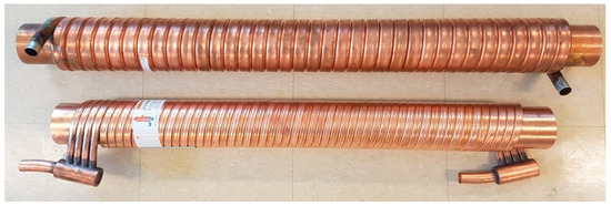
Figure 1.
Common designs for falling-film drain water heat recovery (DWHR) systems.
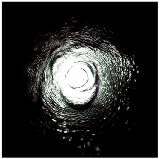
Figure 2.
The falling film in the drain-side pipe for a vertical installation.
DWHR systems are becoming more common in residential buildings, and as such, the building codes and incentive programs are updated to include them. In Canada, the Governments of Ontario and Manitoba have updated their provincial building codes to mandate the installation of these systems in new residential buildings [6,7]. The Canada Green Building Council has also incentivized the use of DWHR systems by making it possible to receive a point towards the Efficient Domestic Hot Water Equipment credit in the LEED Canada for Homes 2009 rating system [8]. Lastly, the Canadian Standards Association (CSA) has produced standard B55.1–15, which is widely used by the manufacturers for rating the performance of DWHR systems [9].
Water heating demand can be reduced significantly through the use of a DWHR system. A study by the Manitoba Advanced House in Winnipeg, Canada, estimated that 50% of a typical family’s annual domestic hot water load could be recovered [10], and a subsequent study by Oak Ridge National Labs produced similar results [11]. Later research conducted by the Canadian Centre for Housing Technology examined DWHR systems and concluded that gas consumption for water heating could be reduced by 9% to 27% depending on the system configuration [12]. More recently, long term simulations of DWHR systems done by Mazur and Słyś showed reductions in annual domestic water heating demands by 23–31%, as well as significant potential to reduce CO2 emissions [13,14]. Other studies conducted in Canada and the Netherlands support these results [15,16].
Each of the previously mentioned studies focused only on proving the feasibility of using DWHR systems to reduce energy consumption. None attempted to produce performance models for DWHR systems. Significant efforts have been made to address this issue at the University of Waterloo through a series of studies. The first study aimed to develop the characteristic effectiveness vs. flow rate curves for multiple DWHR systems [17], while others investigated the impacts of drain-side wetting [18], off-vertical system installation [19], variable inlet temperatures [20] and unequal flowrates [21]. The results from these studies were combined into a preliminary model capable of predicting the steady-state performance of DWHR systems using data obtained from the CSA’s rating process, which was presented at a conference in 2016 [22]. This work aims to fully present the model and the conditions for which it was developed, discuss the need for its validation to cover conditions that were not included during model development, and show that the model still remains pertinent for such conditions.
2. Method
DWHR systems are rated based on their effectiveness using the ε-NTU method, where represents the effectiveness, and NTU represents the Number of Transfer Units [9,23]. By this method, the effectiveness, , is defined as the ratio of heat transfer, , to the maximum heat transfer, , which can occur in the heat exchanger. This effectiveness is expressed as shown in Equation (1).
where represents the heat capacity rate (kW/°C), m is the mass flow rate (kg/s), is the specific heat (kJ/kg°C), and is the temperature (°C). The subscripts c and h refer to the cold mains side and warm drain side, while i and o refer to the inlet and outlet. Lastly, the subscript min refers to the lesser of and .
The CSA standard requires effectiveness to be measured only under equal flow conditions, and assumes the properties of water are constant on both sides of the heat exchanger [9]. As a result, Equation (1) can be simplified, and a DWHR system’s equal flow effectiveness can be determined using Equation (2). Since the purpose of a DWHR system is to preheat the cold mains-side water, the effectiveness is always calculated based on the mains-side temperatures.
Equation (2) is mandated for rating DWHR systems according to CSA standard B55.1–15 [9]. It dictates that the system effectiveness be evaluated for a mains-side temperature of 12 ± 0.4 °C, a drain-side temperature of 28 ± 0.6 °C above the mains-side temperature, and at six volumetric flow rates: 5.5, 7, 9, 10, 12 and 14 L/min. A curve fit of the form shown in Equation (3) is then fit to the data. The curve fit is then used to produce a single rated effectiveness value at 9.5 L/min, which is the metric used for selling DWHR systems on the market.
where (min/L) and (dimensionless) are fit coefficients, and is the volumetric flow rate in L/min.
An apparatus for testing the performance of DWHR systems was constructed at the University of Waterloo. Inlet and outlet water temperatures on both sides of the heat exchanger can be measured using immersion resistance temperature detectors to within ±0.1 °C. Tests can be performed for volumetric flow rates of up to 26 L/min with a reading accuracy of ±1%. The system is set up to permit testing under both equal flow and unequal flow conditions.
A simplified schematic of the test setup is shown in Figure 3. In the figure, the black lines represent the components in the system that are involved in the normal operation of the system when the DWHR unit is being operated under equal flow conditions. This is achieved using a single positive displacement vane pump to push water through the entire system in a single flow path, which ensures that the mass flow rates through both sides of the heat exchanger are equal. To achieve unequal flow conditions during tests, bypass branches equipped with solenoid valves have been implemented in the test apparatus, which are shown using red and blue colors on Figure 3. The blue branch is activated for test conditions when a lower flow rate is desired on the hot side of the heat exchanger relative to the cold side. Conversely, the red branch is activated to achieve higher flow rates through the cold side relative to the hot side. Furthermore, anti-stratification measures have been incorporated into the test apparatus to ensure constant inlet water temperatures during testing. A detailed description of this apparatus is available online [24].
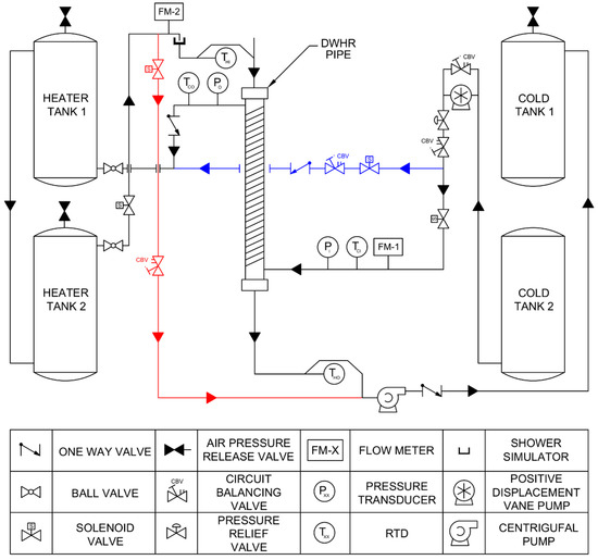
Figure 3.
Simplified schematic of the test apparatus during operation, where the blue and red branches allow variation in flow rates on the cold and hot side of the DWHR unit respectively.
3. Model Development
Based on the authors’ experiences in testing DWHR systems, a multistep strategy was laid out for using data obtained from the rating process, to estimate steady-state performance under real operating conditions. In short, one must first estimate the equal flow effectiveness for the DWHR system, correct it for the inlet fluid temperatures and, if needed, use this to predict the unequal flow performance. Each step will be described in this paper.
3.1. Estimating the Rated Equal Flow Effectiveness Curve
To estimate the equal flow effectiveness curve, some data related to the DWHR system performance are needed. Two likely data sources are presented:
- The user may have access to CSA test data from a system manufacturer, or from CSA reports. If available, these data would contain the equal flow effectiveness curve fit in the form of Equation (3);
- The user may have equal flow effectiveness measurements taken at the CSA test flow rates of 5.5, 7, 9, 10, 12 and 14 L/min, or similar data produced from other sources. The equal flow effectiveness curve can be developed by fitting Equation (3) to these data. Care must be taken when doing this. At low flow rates, the falling film on the drain side becomes unstable and, as a result, the steady-state performance varies between DWHR systems. Therefore, when generating the curve fit, the user is advised not to use any data obtained at flow rates below 5.5 L/min, or below 7 L/min for DWHR systems with diameters of 10.2 cm or larger.
Option (2) is the process specified in the CSA standard to generate the equal flow effectiveness curve mentioned in Option (1). Figure 4 shows an example of the curve fit for the 5.1-cm diameter, 91-cm-long system.
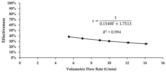
Figure 4.
Equal flow effectiveness vs. flow rate for a 5.1-cm diameter, 91-cm-long DWHR system.
3.2. Temperature Adjustment of the Equal Flow Effectiveness Curve
Previous work showed that variations in the inlet temperatures had an impact on the measured effectiveness for DWHR systems [20]. A theoretical analysis of heat transfer in DWHR systems was also conducted and successfully used to predict the impact of inlet temperatures on system effectiveness [24]. Additionally, this work showed that the change in effectiveness is primarily due to changes in dynamic viscosity with temperature, and the resulting impact of this on heat transfer coefficients. It is evident that the inlet temperatures used during the production of the equal flow effectiveness curve are important, as is the correction of the curve to suit the conditions being studied by the user.
A temperature correction scheme could be developed based on the aforementioned theoretical analysis, but it was deemed to be overly complex. Instead, it was decided that a simpler correlation could be developed based on experimental data. This correlation is shown in Equation (4).
where is the equal flow effectiveness at a set of known inlet temperatures, is the equal flow effectiveness determined at a set of inlet reference temperatures, and is the correction factor. All temperatures are in °C. The reference temperatures were chosen to be = 40 °C and = 10 °C. More details about the development of Equation (4) can be found in previous publications [20,24].
3.3. Performance at Unequal Flow Conditions
The final step needed for determining system performance is to examine conditions of unequal flow. A semi-empirical correlation was experimentally developed to predict the heat transfer rate at unequal flow rates using heat transfer rate measured at the equal flow condition [21]. This correlation is presented in Equation (5).
where is the heat transfer rate at the unequal flow condition, is the heat transfer rate at the equal flow condition, is the flow rate through the coils and is the flow rate of the falling film. Detailed descriptions of these tests can be found in previous publications [21,24].
4. Overall Model
Using the methods presented in Section 3, it is possible to predict the steady-state performance of a DWHR system based on equal flow data. The overall model combines these methods in the order presented in this section. A complete example will be presented later in Section 4.2. The steps for applying the model are as follows:
- Obtain the equal flow effectiveness curve. The curve may be directly available from CSA reports. If not, fit a curve of best fit in the form of Equation (3) to the equal flow data from CSA or an equivalent rating process. The user is advised not to use any data obtained at flow rates below 7 L/min for DWHR systems with diameters of 10.2 cm or larger, or flow rates below 5.5 L/min for DWHR systems with smaller diameters. Use this curve fit to calculate the equal flow effectiveness at the desired mains-side flow rate;
- Adjust the calculated effectiveness to represent the input temperatures being considered using Equation (4). This is a two-stage process. If the effectiveness curves determined in step (1) are not taken from the reference condition of = 40 °C and = 10 °C, then Equation (4) must first be used to determine . Following this, Equation (4) is used again to calculate at the inlet temperatures of interest;
- A conversion from effectiveness to heat transfer rate is required. Make the conversion using Equation (6), where is the flow rate in L/min, the heat transfer rate, q, is in kW, and temperatures are in °C. The numbers in Equation (6) assume constant fluid density ( = 1000 kg/m3) and specific heat ( = 4.18 kJ/kg°C) for water. The 60,000 in the denominator is to convert from L/min into m3/s.
- If required, find the unequal flow heat transfer rate using Equation (5).
This procedure was developed for DWHR systems with mains-side inlet temperatures between 5 °C and 20 °C, drain-side inlet temperatures between 25 °C and 45 °C, and flow rates between 5.5 L/min and 14 L/min, except for systems with diameters of 10.2 cm or larger, where the valid flow rates are between 7 and 14 L/min.
4.1. Model Limitations
As summarized in the previous paragraph, the model was developed for a limited range of inlet flow rates and temperatures. The performance of DWHR systems is a strong function of inlet flow rates, and the range of flow rates chosen for model development were adapted from those covered in the CSA standard [9]. The validation for the model in this range of flow rates was presented in 2016 [22].
The range of flow rates for which the model was validated is insufficient to cover what occurs in many plumbing systems where DWHR systems are installed. To clarify this statement, Figure 5 was created to show three distinct plumbing systems containing a DWHR pipe. The three variations shown in the figure are simplified to only contain a showerhead for water-drawing purposes and, to better represent a realistic case scenario, each showerhead is equipped with a mixing valve. In the figure, is the temperature, is the volumetric flow rate, and properties are assumed to be constant. Figure 5A depicts a system where all preheated water from the DWHR pipe is fed to the water heater, Figure 5B depicts a system where all preheated water is fed to the mixing valve at the showerhead, and Figure 5C shows a combination of the two.
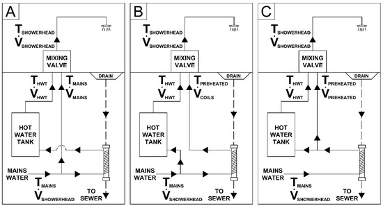
Figure 5.
Possible plumbing setups for DWHR systems in a residential building. In the figure, (A) depicts a system where all preheated water from the DWHR pipe is fed to the water heater, (B) depicts a system where all preheated water is fed to the mixing valve at the showerhead, and (C) is a combination of (A,B).
For all three cases shown in Figure 5, and considering that a typical showerhead has a flow rate of 9.5 L/min (2.5 gallons/min), if two or more shower events occur simultaneously, the total flow rate exceeds the maximum flow rate for which the model was validated. This situation could apply to high-rise residential buildings, college dormitories, gymnasiums, and any other application where the flow rate of drain water exceeds 14 L/min. Clearly, further investigation is required to determine if the model still works for flow rates higher than 14 L/min.
It is also possible for the flow rate through a DWHR system’s coils to fall below the lower limit of the model, even for a typical showerhead flow rate of 9.5 L/min. Consider the following case for plumbing setup depicted in Figure 5A: the showerhead flow rate is fixed at 9.5 L/min, the mains temperature is 10 °C, the user chooses a shower temperature of 35 °C, and the hot water tank’s temperature is a typical 60 °C. Ignoring all losses, and by performing mass and energy balances on the mixing valve, the volumetric flow rate of water going through the DWHR system’s coils can be calculated. In this case, the flow rate was determined to be 4.75 L/min, which fell below the lower limit for which the model was validated. This exercise was then repeated for the same showerhead flow rate of 9.5 L/min, for constant mains water temperatures of 5, 10 and 15 °C, and shower temperatures varying from 15 to 45 °C. The results are shown in Figure 6, where the straight lines represent constant mains temperatures as labelled, and the shaded area enclosed by dashed lines represents the region in which the model was developed.
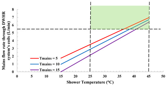
Figure 6.
Mains water flow rate through the DWHR system as a function of shower temperature for a 9.5-L/min showerhead, for constant mains water temperatures of 5, 10 and 15 °C.
Many of the extremely low flow rates shown in Figure 6 correspond to unrealistic conditions, such as 1 L/min corresponding to a shower temperature of 20 °C with a mains temperature of 15 °C. Regardless, additional validation is clearly required to evaluate the model’s capability to predict accurate performance metrics for DWHR systems with flow rates below 5.5 L/min through their coils.
4.2. Model Validation
Before the model could be implemented into building simulation software, it had to be validated to address the limitations described in Section 4.1. To do so, eight different DWHR pipes representing three different diameters and two different manufacturers were selected for testing. Table 1 lists the systems examined.

Table 1.
DWHR systems tested for validation.
To produce performance data equivalent to those from the CSA rating [9], the eight systems were tested at equal flow rates of 5.5, 7, 9, 10, 12 and 14 L/min, and at inlet temperatures of 40 ± 0.5 °C and 12 ± 0.5 °C on the drain side and the mains side, respectively.
Each system was then tested under many different inlet conditions to produce data for the validation process. Mains inlet temperatures were between 4 and 22 °C, while the drain inlet temperatures were between 25 and 50 °C. Note that some of the inlet temperatures used for these tests were outside of the range for which the model was developed; this was done to determine whether the model remains accurate for such temperatures. The drain side flow rates were between 7 and 20 L/min for DWHR systems with a diameter of 10.2 cm, or between 5.5 and 20 L/min for systems with smaller diameters. The validation of the model for drain side flow rates lower than the ones listed above was not attempted in this work for two reasons. Firstly, in typical installations, this flow rate is dictated by the showerhead flow rate, which is usually above 5.5 L/min; secondly, the falling film becomes unstable and sometimes breaks apart at very low flow rates. As for the mains side flow rates, the range of flow rates in this study were between 4 and 20 L/min. The lower bound of 4 L/min was chosen mainly because the test apparatus is unable to hold a steady flow rate below 4 L/min.
In total, over one hundred validation cases were considered, and for each case, the predicted performance was compared to the measured result. Due to the sheer volume of data, it was deemed necessary to first show an example for how the model is applied to the validation cases. The calculation procedure is demonstrated here for one of these cases. The 5.1-cm diameter and 91-cm-long DWHR system (System #1) was first tested to produce the CSA-equivalent data listed in Table 2. The data from Table 2 were used to generate a curve fit in the form of Equation (3) to characterize the effectiveness as a function of the flow rate, as shown in Equation (7).
Table 2.
Canadian Standards Association (CSA)-equivalent data for System #1.
The system’s performance was then evaluated at random conditions, one of which had = 4.7 °C, = 47.3 °C, a mains-side flow rate of 3.97 L/min, and a drain-side flow rate of 7.97 L/min. The measured steady-state heat transfer rate for this test was 6.25 kW.
Following the procedure described at the beginning of Section 4, the first step is to obtain the equal flow effectiveness curve for this DWHR system, shown in Equation (7), and use it to predict the equal flow effectiveness at the mains-side flow rate, as shown in Equation (8).
This effectiveness must then be adjusted for temperature in a two-stage process. First, the reference effectiveness is calculated using Equation (4). The CSA-equivalent tests were performed at = 12 °C and = 40 °C; therefore, the reference effectiveness is calculated as shown in Equation (9).
Solving the above equation gives a value of = 0.4213. The next stage is to use in Equation (4) to determine the effectiveness at the inlet temperatures of = 4.7 °C, = 47.3 °C as shown in Equation (10).
Solving this gives a temperature-corrected equal flow effectiveness value of = 0.4238. Using Equation (6), this effectiveness is then converted to a heat transfer rate, as shown in Equation (11).
This heat transfer rate corresponds to the equal flow condition, and since the flow rates in the validation case were not equal, Equation (5) must be used. The unequal flow calculation is shown in Equation (12).
where = 6.19 kW is the predicted heat transfer rate for the validation case. This is 0.06 kW lower than the measured value of 6.25 kW, with a prediction error smaller than 1% for this example.
A total of 135 validation tests were performed, 93 of which had at least one inlet flow rate outside of the CSA range of flow rates. The predicted heat transfer rates for all DWHR units were plotted against the measured values, as shown in Figure 7, for all 135 validation cases. The identity line of y = x, which represents a perfect model, was also drawn on the figure to visually highlight the model’s inaccuracies. It can be seen in the plot that the test results lie in close proximity to the y = x line, even when the flow rates were outside the bounds in which the model was developed. It is worth noting that, on average, the results were more erroneous for cases with flow rates outside of the CSA range. This can be attributed to the fact that the curve fit used in the first step of the model is based on the range of flow rates prescribed by the CSA standard.
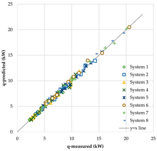
Figure 7.
Predicted vs. measured heat transfer rates for all 135 test cases.
To provide an estimate for the prediction errors associated with the model, the Mean Absolute Percentage Error (MAPE) associated with the results was calculated using Equation (13). MAPE represents the error as a percentage, and eliminates the scale dependency of the outcome. The MAPE was calculated to be 3.47% for the case with 93 non-CSA flow rates, and the MAPE for the entire data set was 2.96%. Table 3 summarizes the statistical results, as well as the maximum prediction errors between the measured and predicted heat transfer rates.
Table 3.
Comparison of model’s accuracy for different flow regions.
The results listed in Table 3 showed that the model, on average, was almost twice as erroneous when it was used to predict heat transfer rates outside of the CSA’s range of flow rates. The increased errors in model predictions were not large enough to require the development of a new model from scratch; however, the CSA rating process can be modified to improve the predictions. Recall that the main input to the model, which specifies the DWHR system, is the characteristic effectiveness vs. flow rate curve developed during the CSA rating procedure. The curve fit used in the model is based on the range of flow rates prescribed by the CSA standard, which then gets extrapolated to predict performance at flow rates outside this range. The model cannot account for errors caused by extrapolating the curve fits; instead, it stands to reason to expand the CSA standard’s range of flow rates to include additional data points in order to generate better curve fits, and eliminate the need for extrapolation.
5. Discussion
The model presented in this work is intended to be incorporated into building simulation models where detailed information about water usage and the plumbing system are known. However, this model addresses some of the largest gaps in the literature for accurate simulations of DWHR systems. Currently, annual simulations are based upon a constant effectiveness value (i.e., constant flow rates and temperatures through the heat exchanger), and for plumbing setups similar to what was shown in Figure 5C where the flow rates through both sides of the heat exchanger are equal. Even the most recent studies, such as Mazur’s study from 2018, suffer from such limitations [14]. The model presented in this work allows for the simulation of DWHR systems installed in any of the setups shown in Figure 5 and operated under any flow rates or temperatures.
One of the main advantages of the model is that it can be used to choose an optimal plumbing configuration that could result in maximum savings on an annual basis. This was not possible before, as plumbing configurations can vary significantly, as shown in Figure 5, and robust models are required for optimization purposes. Another advantage of the model is that it could be combined with other technologies to simulate complex systems. For example, a DWHR unit can be installed in a system equipped with solar thermal panels, where it is important to keep track of temperatures for accurate simulations of the system, which is made possible with the model presented in this work.
6. Conclusions
Several DWHR systems, representing different diameters, lengths and manufacturers, were tested as part of the work presented. Methods were developed and validated for determining the equal flow effectiveness curve, to correct for inlet temperatures, and to predict the impact of unequal flow conditions. In each case, these corrections turned out to be independent of diameter, length and coil design.
These methods were combined into an overall model which can predict the steady-state performance of DWHR systems at different conditions. The model was used to predict the heat transfer rates for 135 validation cases, 93 of which had at least one inlet flow rate outside of the CSA standard’s range of flow rates. Model predictions were in good agreement with the measured values, and the mean absolute percentage error for the entire data set was 3%. It was concluded that the model could be used to accurately predict the performance of DWHR systems operating under steady-state conditions.
Author Contributions
Conceptualization, R.M. and M.R.C.; data curation, R.M.; formal analysis, R.M.; funding acquisition, R.M. and M.R.C.; investigation, R.M.; methodology, R.M. and M.R.C.; project administration, M.R.C.; resources, M.R.C.; supervision, M.R.C.; validation, R.M.; writing—original draft, R.M.; writing—review & editing, R.M. and M.R.C. All authors have read and agreed to the published version of the manuscript.
Funding
This research was funded by the Natural Sciences and Engineering Research Council of Canada (NSERC) and the Ontario Graduate Scholarship (OGS) program.
Conflicts of Interest
The authors declare no conflicts of interest.
References
- NRCan. Residential Sector, Canada: Secondary Energy Use and GHG Emissions by End-Use. 2017. Available online: http://oee.nrcan.gc.ca/corporate/statistics/neud/dpa/showTable.cfm?type=CP§or=res&juris=ca&rn=2&page=0 (accessed on 20 May 2020).
- Eurostat. Energy Consumption and Use by Households. 28 March 2017. Available online: https://ec.europa.eu/eurostat/en/web/products-eurostat-news/-/DDN-20170328-1 (accessed on 20 May 2020).
- UEIA. Annual Household Site End-Use Consumption in the U.S. February 2018. Available online: https://www.eia.gov/consumption/residential/data/2015/c&e/pdf/ce3.1.pdf (accessed on 20 May 2020).
- Cooperman, A.; Dieckmann, J.; Brodrick, J. Drain Water Heat Recovery. ASHRAE J. 2011, 53, 58–62. [Google Scholar]
- Schmid, F. Sewage Water: Interesting Heat Source for Heat Pumps and Chillers; Swiss Federal Office of Energy SFOE: Bern, Switzerland, 2008. [Google Scholar]
- Ontario Ministry of Municipal Affairs. Supplementary Standard SB-12 Energy Efficiency for Housing. 2016. Available online: http://www.mah.gov.on.ca/AssetFactory.aspx?did=15947 (accessed on 18 September 2017).
- Government of Manitoba. Manitoba Building Code Amendment. The Buildings and Mobile Homes Act. 2015. Available online: http://web2.gov.mb.ca/laws/regs/annual/2015/052.pdf (accessed on 18 September 2017).
- Canada Green Building Council. LEED® Canada for Homes. 2009. Available online: http://www.cagbc.org/cagbcdocs/LEED_Canada_for_Homes_2009_RS+addendum_EN.pdf (accessed on 18 September 2017).
- CSA. B55.1-15 Test Method for Measuring Efficiency and Pressure Loss of Drain Water Heat Recovery Units; Canadian Standards Association: Mississauga, ON, Canada, 2015. [Google Scholar]
- Proskiw, G. Technology Profile: Residential Greywater Heat Recovery Systems; The CANMET Energy Technology Centre (CETC) Energy Technology Branch, Department of Natural Resources Canada: Ottawa, ON, Canada, 1998. [Google Scholar]
- Tomlinson, J.J. Heat Recovery from Wastewater Using a Gravity-Film Heat Exchanger; Oak Ridge National Laboratory: Oak Ridge, Tennessee, TN, USA, 2001. [Google Scholar]
- Zaloum, C.; Gusdorf, J.; Parekh, A. Performance Evaluation of Drain Water Heat Recovery Technology at the Canadian Centre for Housing Technology; Natural Resources Canada: Ottawa, ON, Canada, 2007. [Google Scholar]
- Mazur, A.; Słyś, D. Possibility of heat recovery from gray water in residential building. Sel. Sci. Pap. J. Civ. Eng. 2017, 12, 155–162. [Google Scholar] [CrossRef]
- Mazur, A. The impact of using of a DWHR heat exchanger on operating costs for a hot water preparation system and the amount of carbon dioxide emissions entering the atmosphere. In Proceedings of the E3S Web of Conferences, Krakow, Poland, 7–8 June 2018; Volume 45. [Google Scholar]
- Eslami-nejad, P.; Bernier, M. Impact of Grey Water Heat Recovery on the Electrical Demand of Domestic Hot Water Heaters. In Proceedings of the Eleventh International IBPSA Conference, Glasgow, Scotland, 27–30 July 2009. [Google Scholar]
- Schuitema, R.; Sijpheer, N.C.; Bakker, E.J. Energy Performance of a Drainwater Heat Recovery System. In Proceedings of the European Conference and Cooperation Exchange on Sustainable Energy, Vienna, Austria, 5–8 October 2005. [Google Scholar]
- Collins, M.R.; Van Decker, G.W.; Murray, J. Characteristic effectiveness curves for falling-film drain water heat recovery systems. HVAC&R Res. 2013, 19, 649–662. [Google Scholar]
- Beentjes, I.; Manouchehri, R.; Collins, M.R. An investigation of drain-side wetting on the performance of falling film drain water heat recovery systems. Energy Build. 2014, 82, 660–667. [Google Scholar] [CrossRef]
- Manouchehri, R.; Banister, C.J.; Collins, M.R. Impact of small tilt angles on the performance of falling film drain water heat recovery systems. Energy Build. 2015, 102, 181–186. [Google Scholar] [CrossRef]
- Manouchehri, R.; Collins, M.R. An experimental analysis of the impact of temperature on falling film drain water heat recovery system effectiveness. Energy Build. 2016, 130, 1–7. [Google Scholar] [CrossRef]
- Manouchehri, R.; Collins, M.R. An experimental analysis of the impact of unequal flow on falling film drain water heat recovery system performance. Energy Build. 2018, 165, 150–159. [Google Scholar] [CrossRef]
- Manouchehri, R.; Collins, M.R. Steady-state modelling of falling film drain water heat recovery efficiency using rated data. In Proceedings of the eSim 2016 Building Performance Simulation Conference, Hamilton, ON, Canada, 3–6 May 2016; pp. 159–168. [Google Scholar]
- Kays, W.M.; London, A.L. Compact Heat Exchangers; McGraw-Hill Book Company: Stanford, CA, USA, 1964; pp. 14–20. [Google Scholar]
- Manouchehri, R. Predicting Steady-State Performance of Falling-Film Drain Water Heat Recovery Systems from Rating Data. Master’s Thesis, University of Waterloo, Waterloo, ON, Canada, 2015. [Google Scholar]
© 2020 by the authors. Licensee MDPI, Basel, Switzerland. This article is an open access article distributed under the terms and conditions of the Creative Commons Attribution (CC BY) license (http://creativecommons.org/licenses/by/4.0/).