Net Ecosystem Exchange of CO₂ in Deciduous Pine Forest of Lower Western Himalaya, India

Abstract

Carbon cycle studies over the climate-sensitive Himalayan regions are relatively understudied and to address this gap, systematic measurements on carbon balance components were performed over a deciduous pine forest with an understory layer. We determined annual net carbon balance, seasonality in components of carbon balance, and their environmental controls. Results indicated a strong seasonality in the behavior of carbon exchange components. Net primary productivity (NPP) of pine forest exceeded soil respiration during the growing phase. Consequently, net ecosystem exchange exhibited a net carbon uptake. In the initial phase of the growing season, daily mean uptake was −3.93 (±0.50) g C m⁻² day⁻¹, which maximizes (−8.47 ± 2.3) later during post-monsoon. However, a brief phase of carbon release was observed during peak monsoon (August) owing to an overcast condition. Nevertheless, annually the forest remained as a carbon sink. The understory is extensively distributed and it turned out to be a key component of carbon balance because of sustained NPP during the pine leafless period. Temperature and evaporative fraction exhibited a prime control over the seasonal carbon dynamics. Our observations could lend certain useful insights into the application of coupled climate-carbon cycle models for the Himalaya and ecological functions in the region.

1. Introduction

During the last two centuries, anthropogenic CO₂ emissions and deforestation have increased the surface temperature significantly. The built-up CO₂ in the atmosphere causes global warming, whose future extent will not only depend on the size of future emissions, but also on the development of future carbon (C) sinks of the terrestrial biosphere and ocean. Terrestrial biosphere, together with the ocean help by drawing down more than 50% of the annual anthropogenic CO₂ emissions, and their C sink strength have continuously improved over the past five decades [1]. However, the future trend of C sink largely depends on the responses of terrestrial ecosystems to increasing CO₂ concentrations and climate change [2]. Further, the terrestrial C sink is mostly controlled by the forest ecosystems and associated environmental drivers [3].

The C balance of terrestrial ecosystems can be represented by both the net ecosystem productivity (NEP) and net ecosystem carbon exchange (NEE). The balance between ecosystem respiration (Re) and gross primary productivity (GPP) determines NEE, which can be positive (i.e., carbon source) or negative (i.e., carbon sink). NEP can be represented by the difference between net primary productivity (NPP) and heterotrophic ecosystem respiration. The variability of NEE is tightly coupled with the variations of C balance components, namely, GPP and Re, and their responses to environmental variables and climate [4]. Previous studies have underlined that GPP can be influenced by both environmental (i.e., radiation, rainfall, temperature, vapor pressure deficit (VPD), etc.) and biophysical variables (i.e., leaf area index), whereas, Re is primarily regulated by environmental variables, such as temperature and soil moisture [5,6,7]. Further, the variability of Re can be largely biased by the constraints in night-time respiration data availability [7,8]. Thus, it becomes essential to decipher the variability and controls of individual components of carbon balance to understand mechanisms and processes controlling seasonal and inter-annual variability of NEE.

In particular, processes and mechanisms controlling NEE and their responses to changing environment across the Himalayan ecosystems are usually unknown. Over the last few decades, Himalayan ecosystems have experienced increased temperatures and abrupt changes in the precipitation pattern [9,10]. In view of such rapid environmental change, it becomes imperative to study the components of C balance and to evaluate whether the ecosystem is a carbon source or sink. Ecosystem productivity can be derived from varieties of methods, which have their own applicability, strengths and limitations (such as, atmospheric CO₂ inversion (estimate surface-to-atmosphere net C flux), field inventory and book-keeping models, biogeochemical process-based models, satellite data, and flux tower). This study has utilized a combination of chamber-based and micrometeorological methods for understanding and quantifying NEE to determine the sink–source status along with controlling environmental factors.

The deciduous pine forest, Pinus roxburghii, is a dominant vegetation type in the lower western Himalayan region (elevation: 500–2000 m) and it encompasses 18,650 km² area that represents about 6% of the total forested land of India [11]. Given its climatic (subtropical) and ecological importance, we had investigated the radiation–energy balance and inter–linkages of canopy photosynthesis (Ac), and water fluxes across the seasons [12,13]. The results underlined that the degree of coupling between water and C exchange was stronger during transition phases (post–monsoon and spring seasons) [12,13]. Further, we have investigated seasonal dynamics of canopy and soil respiration fluxes based on in situ field measurements. We observed the temporal dynamics of night-time canopy respiration (Rnc) and soil respiration (Rs) fluxes. Their major controlling environmental factors were identified as air/soil temperature, latent heat flux, VPD, soil moisture, and evaporative fraction (EF) [7]. Results also indicated that carbon processes were ideal only within a narrow range of environmental variables. Ac and Rnc were inversely correlated and respiration increased with EF. Overall, phenology determined the respiration–photosynthesis ratio, and understory removal disturbed the carbon balance [7]. Other than our previous attempts [7,12,13], there were no studies found that characterize carbon exchange over coniferous forest in the region. It is also not clear whether the deciduous pine forest behaves as a carbon sink or source.

Within this perspective, the overarching objectives of this study were: (i) To quantify the components of the carbon balance of deciduous pine forest; (ii) to quantify NEE and determine the sink–source status; and (iii) to attain an in-depth understanding on seasonal carbon exchange dynamics and controls using systematic in situ field measurements coupled with concurrent micrometeorological measurements.

To characterize carbon fluxes in a young, deciduous and homogenously distributed Pinus roxburghii forest ecosystem having an understory (Lantana camara: An invasive shrub), we used 14 months of measured micrometeorological, ecophysiological, and biophysical data comprising an annual growth cycle from November 2010 to December 2011. We employed manually intensive chamber-based up-scaling methodology, however at a longer time-interval (continuous 24 h cycles at a 10-day interval). The chamber-based measurements are extremely useful when individual components of carbon balance and environmental factors or disturbances need to be discerned [14], unlike the flux tower or eddy–covariance (EC) technique [8,15,16]. To the best of our knowledge, this is an initial comprehensive study to characterize environmental controls on seasonal variations of NEE and to quantify carbon balance dynamics (source/sink) using annual time-scale in situ based data.

2. Materials and Methods

2.1. Site Description

The experimental study site was located within the reserve forest at the Forest Research Institute (FRI), Dehradun, India (30°20′04″ N and 78°00′02″ E), having a mean elevation of 640 m. The site has a micrometeorological station having multi-level, slow response sensors on a 13 m long tower to measure sub-hourly radiative–convective flux, state parameters, and sub-surface thermal profiles. The station is designed to measure biophysical (LAI—leaf area index and PAR—photosynthetically active radiation,) and ecophysiological (photosynthesis and respiration) properties of the vegetation and soil. The experimental site covers an area over five hectares (stand density: 1000 stems ha⁻¹). The young (8.5 years old, mean height: 6.5 m, and mean DBH: 13.8 cm) pine represents the overstory, while Lantana camara (Verbenaceae) represents shrub understory cover (an invasive species). The understory was managed and it was cleared during 2010 (October–November). However, the understory started re-growing from April 2011 onwards, and further it was not cleared in order to study the effects of understory cover on ecosystems’ carbon fluxes. To have systematic biophysical and ecophysiological measurements, the site was homogenously divided into nine sampling quadrats (10 m × 10 m) in different directions. The micrometeorological tower was placed centrally [12].

2.2. Climate

The site is located in a heavy rainfall zone in the western Himalaya where a warm-moist environmental condition prevails during the growing season (March–October). Monsoon season is from mid-June to mid-September. Precipitation (P) peaks during July–August, whereas, air temperature (AT) remains highest during April and May (Supplementary Figure S1). Overall, the climate could be considered as more energy-limited than water-limited. However, the water-limitation phase occurs only for a short duration confined to the summer (April–May) months. The soil water content (SWC) ranges from 10% in peak summer days to above 24% during the rainy season (mean of three-soil layer: 0.1 m, 0.2 m, and 0.45 m). Due to the failure of automatic field soil tensiometers, we resorted to manual monthly volumetric samplings from three depths near the tower.

2.3. Ecophysiological Measurements

2.3.1. Night-Time Canopy Respiration (Rnc)

Rnc rates of both overstory (pine) and understory (lantana) were measured from canopy foliage except woody tissues (stem and small branches). Rnc rates were manually but intensively measured at a 10-day interval from 10 November 2010 to 31 December 2011 (for e.g., Nov1d 2010 to Dec3d 2011) for 12 h (1830 to 0530 h LMT18) using the LI–6400 XT portable photosynthesis system (model LI–6400 XT, standard leaf chamber area: 2 cm × 6 cm, LI-COR, Lincoln, NE, USA). For measurements under prevailing environmental conditions (as per the LiCOR instruction manual), block temperature and VPD was maintained under ambient conditions. The airflow rate and reference CO₂ was set at 400 μmol mol⁻¹ and 380 μmol mol⁻¹, respectively [17].

Hourly sampling of the overstory and understory species consisted of 360–450 readings distributed across three plants in three different quadrats, with three to five leaves per vertical layer of a plant around each canopy position (top, middle, and bottom). Each plant was divided into three vertical layers, and only one plant was measured in a sampling quadrat. Within 1.5–2.0 min on each layer, 40 to 50 readings were collected. Accordingly, each plant in a quadrat was sampled for 6 min that provided a total of 120 to 150 readings. Three different quadrats were sampled at each hour for each species (pine and lantana), at 15-min interval, and averaged for that hour. Periodically, valve matching was performed to maintain consistent data quality. The night-time leaf-level respiration data from the photosynthesis system were up-scaled to the canopy level on the basis of LAI measurements [18,19] as well as on the canopy leaf area basis (Section 2.4) [20].

2.3.2. Soil Respiration (Rs)

Using a soil chamber (LI–6400–09) and LI–6400 IRGA (Li–COR, Lincoln, NE, USA), Rs rates were measured for 24 h at a 10-day interval. The LI–6400 IRGA was randomly used in different quadrats in order to acquire the maximum possible spatial coverage. Hourly readings consisted of three measurement points in a quadrat. To check for data quality and to compute measurement uncertainty, the data was supplemented and compared intermittently by applying another closed, static chamber (25 cm × 25 cm) based on an infrared gas analyzer (IRGA) CO₂ sensor (GasAlertMicroIR5, BW Tech., Honeywell Inc., Charlotte, NC, USA). Within a quadrat, systematic sampling was done to cover both the root and non-root zone (based on the distance from trees) to have true representation of Rs (including both soil and root respiration). To avoid real-time effect of disturbance on CO₂ emission, chambers were slipped into the collars inserted to the soil layer 24 h prior to the measurements.

2.3.3. Day-Time Net Canopy Photosynthesis (Ac) and Net Primary Productivity (NPP)

Procedure and periodicity for hourly sampling of leaf-level photosynthesis of the over and understory species were similar as described above for night-time canopy respiration (Section 2.3.1). On each day of measurement, daytime (0600 to 1800 h LMT) net photosynthesis and respiration in the next night (1830 to 0530 h LMT) was measured hourly.

Day-time leaf-level photosynthesis of both the overstory and understory species was measured using the LI-6400 XT photosynthesis system under prevailing environmental conditions. Hourly leaf-level photosynthesis data were upscaled to the canopy-level according to Campbell and Norman [21] assuming single light assimilation responses in relation to all the leaves in the canopy and sunlit and shaded class based on canopy sub-division into the three (top, mid, and bottom) layers. Descriptions of upscaling and associated errors are described in Singh et al. [13]. Thus, it represents day-time net canopy assimilation (Ac). In other words, it was the gross primary production $\left(\mathrm{GPP}\right)$ minus the day-time respiration $(R{d}_{day})$. Mathematically, it can be written as:

$$A_c=\mathrm{GPP}-R{d}_{day}$$

(1)

Given the strong inhibition of day-time respiration [8] in light conditions and lower level of day-time respiration with respect to night-time respiration [22,23]; and thus, contribution of day-time respiration in total daily canopy respiration, Ac has been assumed equivalent to the gross primary productivity (Ac ≈ GPP). Daily net primary productivity (NPP) was computed by subtracting Rnc from Ac [24]. Mathematically, it can be expressed as:

$$\mathrm{NPP}=A_c-R_{\mathrm{nc}}$$

(2)

Therefore, daily net ecosystem exchange (NEE) becomes:

$$\mathrm{NEE}=R_{\mathrm{s}}-\mathrm{NPP}$$

(3)

where, $R_{\mathrm{s}}$ is soil respiration (heterotrophic and root respiration).

NEE is an indicator of net carbon balance of the ecosystem. Negative sign denotes a net carbon flux from atmosphere to ecosystem (i.e., carbon sink), and thus a net carbon uptake by the ecosystem. As it is a derived flux, thus, we computed the standard error (s.e.) associated with NEE to represent the magnitude of variations.

$$\mathrm{SE}=\sqrt{{\mathrm{SE}}_{\mathrm{NPP}}{}^2+{\mathrm{SE}}_{R\mathrm{s}}{}^2}$$

(4)

where, ${\mathrm{SE}}_{\mathrm{NPP}}$ is the s.e. of NPP; while ${\mathrm{SE}}_{R\mathrm{s}}$ is the s.e. of Rs.

Carbon use efficiency (CUE) was computed as the ratio of daily integrals of NPP to Ac (≈GPP) that signifies the capacity of plants to transfer carbon from atmosphere to terrestrial biomass [25]. It is a dimensionless index of carbon flux efficiency from the atmosphere to the vegetation (range: 0 to 1). Values closer to 1 is indicative of a higher carbon flux efficiency from atmosphere to vegetation.

2.4. Biophysical Measurements: LAI and Phenology

Concurrent to the ecophysiological measurements, leaf area index (LAI) was also measured at a 10–day interval in overstory pine throughout the study period, while the LAI was measured in the understory after growth initiation (i.e., March 2011 onwards). We used a plant canopy analyzer (PCA) (LAI-2000; Li-COR, Inc., Lincoln, NE, USA) for measuring LAI. A detailed sampling plan and correction factor (1.57) for the clumping of needles in the pine canopy were described in Singh et al. [13]. Overall, we followed the procedure as per the PCA LAI-2000 instruction manual.

Annual phenology of the pine exhibited a distinct green and brown stage. The transition dates from one growth stage to another of pine and lantana were monitored using digital field photographs and visual observations. With the onset of spring season and increasing temperature physiological activities in pine (i.e., emerging green needles) were manifested. Canopy greening was complete by the month of May. It remained green until October, while canopy browning started with the onset of the winter season (November–February). The understory (lantana) was cleared in October 2010 as a part of management practice. After the arrival of spring (March) in 2011, new leaves began to re-appear from its tuberous underground root. By the end of March, lantana attained an average height of 0.6 m. Its canopy was fully developed before the onset of monsoon with a mean height of 1 m. In the next winter (2011), when lantana was not cleared, sign of leaf browning was observed in the winter.

2.5. Micrometeorological Observations and Data Processing

An INSAT uplinked micrometeorological tower (13 m) was installed within the homogenously distributed young pine forest with a fetch of about 500 m from all directions (fetch ratio = 1:100) for continuous and automated measurements of radiation components (shortwave and longwave), energy and water balance. The slow response sensors consisted of a four component net radiometer (at 10 m; Kipp and Zonen, Delft, Netherlands), two-depth (at 0.1 m and 0.2 m) self-calibrating soil heat flux plates (HFP-01SC, Radiation & Energy Balance System Inc., Bellevue, WA, USA), three-height (at 4.5 m, 7.5 m, and 12.5 m) air temperature–relative humidity (AT—RH) probes with a shielded and aspirated sensor (HMP-45C, Campbell scientific, Logan, UT, USA), three-height (at 4.5 m, 7.5 m, and 12.5 m) anemometer-vane for wind speed and direction (KDS-131, Komoline Aerospace Limited, Ahmedabad, India), and three-depth (0.05 m, 0.2 m, and 0.45 m) soil thermometers (KDS-031, Komoline Aerospace Limited, Ahmedabad, India). A rain gauge of the tipping bucket type (KDS-071, Komoline Aerospace Limited, Ahmedabad, India) was placed in the open to record rainfall. A programmable 25-channel data logger (DSAWSKM1-W, Komoline Aerospace Limited, Ahmedabad, India) automatically stored these data. The data were logged every second and averaged for 30 min [12].

Batch processing of micrometeorological data was carried out to convert all sub-hourly fluxes into daily averages. Radiation balance components and ground heat flux were averaged for the daytime and for the 24 h period. 10-day (dekadal) and monthly averages of fluxes were computed from daily averages. The data quality was screened to remove spurious spikes in the instantaneous and daily averages to have smooth temporal transition [26] and to obtain reliable dekadal averages.

Net radiation at the surface was computed from the four components of radiation balance as given in Equation (5).

$$R\mathrm{n}={\mathrm{SW}}_{\mathrm{net}}+{\mathrm{LW}}_{\mathrm{net}}$$

(5)

where,

$${\mathrm{SW}}_{\mathrm{net}}=\mathrm{SW}\downarrow -\mathrm{SW}\uparrow$$

$${\mathrm{LW}}_{\mathrm{net}}=\mathrm{LW}\downarrow -\mathrm{LW}\uparrow$$

where, SW and LW are shortwave and longwave radiation, respectively. The symbols ‘↓’ and ‘↑’ represent incoming and outgoing fluxes, respectively. The SWnet and LWnet are net shortwave and net longwave radiation fluxes at the surface. The net radiation (Rn) is partitioned into sensible heat flux (SH), latent heat flux (LE), ground heat flux (G), and metabolic and storage energy in the vegetation canopy (ΔH).

$$R\mathrm{n}=\mathrm{SH}+\mathrm{LE}+\mathrm{G}+\Delta \mathrm{H}$$

(6)

G was measured following methodology adopted by Heusinkveld et al. [27]. The storage heat of the canopy was ignored in the seasonal cycle, with the assumption that the amount of energy stored during the heating cycle is being released during the cooling cycle [26]. The amount of metabolic heat is usually negligible as compared to other components [26].

The net available energy (Q) was computed as:

$$\mathrm{Q}=R\mathrm{n}-\mathrm{G}$$

(7)

Latent heat flux from Bowen ratio energy balance (BREB) method was computed as:

$$\mathrm{LE}=\frac{R\mathrm{n}-\mathrm{G}}{1+\mathsf{\beta }}$$

(8)

where: $\mathsf{\beta }=\frac{\mathrm{SH}}{\mathrm{LE}}=\mathsf{\gamma }\frac{{dT}_a}{{de}_a}$

The air temperature ($\frac{d{T}_a}{dZ}$) and vapor pressure ($\frac{d{e}_a}{dZ}$) gradients can be determined through multi-height measurements within the surface layer (or quasi-laminar boundary layer). γ is the psychrometric constant (0.66 mbar °C⁻¹).

The evaporative fraction (EF) was computed as the ratio between the evapotranspiration (LE) and the available energy (Q) at the land surface and considered as an indirect indicator that affects the C balance. It is a stable indicator of the annual dryness–wetness cycle that isolates surface control (soil moisture and vegetation) from radiation and turbulent factors (range 0 to 1). EF is thus supposed to be a diagnostic of the surface energy balance that is constant or self-preserved and it is a characteristic physical parameter, which defines ecosystems into two broad categories: (1) Energy-limited and (2) water-limited regime [28]. In the energy-limited regime, EF is independent of the soil moisture content, while it provides a first-order constraint in water-limited condition. Stronger evapotranspiration (ET) and AT relationship than evapotranspiration and vapor pressure deficit (ET–VPD) relation [13], defined this subtropical pine ecosystem as energy-limited rather than water-limited that prompted us to analyze its interrelationship with ecophysiological variables.

2.6. Statistical Analysis and Uncertainty Estimate

Pearson’s correlation analysis was conducted to examine the relationship between carbon cycle components and environmental-biophysical factors. Additionally, a one-to-one interaction between significantly correlated carbon components and environmental-biophysical predictors were assessed using a linear regression analysis. Further, we used multiple regression and an ANOVA to identify the best environmental-biophysical factors as predictor variables. Significant statistical differences were set with p < 0.001, unless otherwise stated. All statistical analyses were performed using SPSS (ver. 14) software (IBM, Bangalore, India). We further explored the possibility of the temporal relationship between carbon fluxes and environmental-biophysical drivers influencing these C-balance components using a wavelet coherence analysis [29]. Analyses were performed using MATLAB R2012 (The MathWorks, Inc., Natick, MA, USA) and wavelet analysis software [29,30].

3. Results

3.1. Environmental Variables and Seasonal Variations

Typical western Himalayan subtropical climatic condition is interesting and worth highlighting (

Table 1. Mean climatic (subtropical) and soil characteristics of the study site.

Variables	Characteristics	Remarks
Annual Rainfall	2020 ± 423 mm	Average over 1940–2010, Peak during July–August
Air Temperature	11.5 °C (January), 27 °C (June)	Peak during May–June
Humidity	52% (April), 85% (August)	Lowest (summer season), Maximum (rainy season)
Sunshine	4.4 h day−1 to 9.3 h day−1	Minimum (July–August), Maximum (May)
Pan Evaporation	1.2 mm to 7.2 mm	Minimum (December), Maximum (May)
Vapor Pressure Deficit (VPD)	0.37 kPa to 3.7 kPa	Lowest (monsoon), Highest (summer)
Soil Moisture	10% to 24% (mean of the three-soil layer: 0.05 m, 0.2 m, and 0.45 m)	Lowest in May (summer), Maximum (rainy season)
Soil type	Mollisols	3–8 m thickness, Porosity 40–60%
Soil Texture	Sandy clay loam	35% sand, 40% clay, and 25% silt
Soil pH	4.5–6	Acidic
Bulk density	1030 kg m−3	0–20 cm depth

). The study site lies in a heavy rainfall zone in the western Himalayan region (70-year average: 2020 ± 423 mm). The seasonal pattern of temperature (AT), precipitation (P), matched concurrently with peaks of both P and AT (mean 25.5 °C) occurs during July–September (Figure S1). Such coincident variation (warm-moist condition) is the environmental characteristic of the region. Vapor pressure deficit (VPD: 1.1 ± 0.85 kPa) remained high (3.7 kPa) only during the dry summer (April–May) and at a minimum (0.37 kPa) during the monsoon. Soil water content varied between 11% (May) and 24% (August). Sunshine hours varied from 4.4 h day⁻¹ to 9.3 h day⁻¹ with a minimum during July–August and maximum during May. The mean monthly open pan evaporation varies from 1.2 mm to 7.2 mm with the lowest during winter and the highest during summer. Seasonal VPD and soil moisture dynamics were found inversely but significantly related (R² = 0.69, p < 0.001). Evaporative fraction (EF: The ratio between the evapotranspiration (ET) and the available energy at the land surface), an indirect indicator of the annual dryness–wetness cycle (range: 0–1), remained above 0.38 throughout the study period with a mean of 0.58 ± 0.16. It was lowest (0.38) during winter and highest (0.9) during the monsoon. Further, the stronger ET and AT relationship than the ET–VPD relation defined this subtropical pine ecosystem as energy-limited rather than water-limited. The energy and water limitation phase during an annual growth cycle occurs in a continuum with a shorter water limited period (confined only to the summer months: April–June; Figure S2).

3.2. Seasonal Variations in NPP, Rs, and NEE

The behavior of carbon fluxes (NPP, Rs, and NEE) across the seasons such as winter 2010 (no understory), pre- and post-monsoon (comprising the growing period: April–October), and winter 2011 (with understory) has been shown in Figure 1. With the advent of the growth conducive spring season, the increment in NPP was remarkable. It attained peak in the post-monsoon season (23.6 μmol CO₂ m⁻² s⁻¹). Results also indicated a dropdown in NPP from July3d (10 day intervals: 21–30 July) to Aug3d (21–30 August) that has been attributed to decline in photosynthesis owing to an overcast condition during the rainy season (i.e., limited incoming solar radiation input including PAR). The mean NPP over the growing period (April–October) was observed at 11.75 ± 1.25 (s.e.) μmol CO₂ m⁻² s⁻¹ (CV: 49%). NPP was minimum (0.7 ± 0.14) during winter 2010 (no understory and dormant overstory), while it was almost 11 times higher during winter 2011 (7.9 ± 1.96 μmol CO₂ m⁻² s⁻¹) due to the presence of an understory.

The annual cycle of soil respiration (Rs) was bimodal (Figure 1). With leaf onset during spring (March–April), a smaller peak (7–8 μmol CO₂ m⁻² s⁻¹) was noticed. Rs attained peak in the post-monsoon season (12–15 μmol CO₂ m⁻² s⁻¹; Figure 1). Mean Rs over the growing period was 9.2 ± 2.8 (s.e.) μmol CO₂ m⁻² s⁻¹ (CV: 30%). Rs rates declined with the advancement of summer owing to water limitation (or declined soil moisture). Thereafter, it increased with the arrival of monsoon and again declined during winter. During winter 2010 and 2011, Rs rates were 6.3 ± 0.17 and 7.25 ± 0.24 μmol CO₂ m⁻² s⁻¹, respectively. The coefficient of variation (CV) in these periods were 10.7% and 8.2%, respectively, reflecting a feeble role of photosynthates from the understory and overstory on Rs during the winter physiological state.

NEE varied to a large extent during the observational period that ranged from −12.8 μmol CO₂ m⁻² s⁻¹ to 6.3 μmol CO₂ m⁻² s⁻¹, with an average of −3.3 ± 1.65 (s.e.) μmol CO₂ m⁻² s⁻¹ over the peak growing period (June–October). NEE was negative (carbon sink) mostly over the growing period (Figure 1). However, within the growing period, NEE attained a positive level (carbon source) in the peak monsoon season (July3d–Aug3d), owing to response of carbon processes to ambient environmental conditions. As described earlier, this was mostly attributed to the overcast condition. Outside the window of July3d–Aug3d, NEE continued as a carbon sink, with an average of −6.3 ± 1.3 μmol CO₂ m⁻² s⁻¹. A peak in the carbon sink was observed during post-monsoon season (September–October) when the clear sky condition prevailed with abundant soil moisture. Due to the physiological dormancy of pine during winter 2010 when the understory was removed, NEE was observed as a carbon source, with an average of 5.57 ± 0.23 μmol CO₂ m⁻² s⁻¹. Whereas, during the winter 2011 (with the understory layer), the ecosystems became a net sink of CO₂, with an average of −0.66 ± 1.72 μmol CO₂ m⁻² s⁻¹. Higher s.e. observed during winter 2011 might be due to less observations (n = 6, representing November–December), while winter 2010 had more observations (n = 12, representing November to February). Nevertheless, the substantial difference in the winter season NEE fluxes could be attributed to the presence of an understory (lantana). The effect of understory removal was exhibited until the spring–summer period of 2011. During this period both understory and overstory canopy was still developing and the ecosystem exhibited a carbon source (3.96 ± 1.0 μmol CO₂ m⁻² s⁻¹).

These results underlined that the removal of the understory has disturbed an aspect of the carbon balance of this ecosystem. The ecosystem was found to be a source of carbon when understory was absent for about five months (November 2010–March 2011). The understory (Lantana camara: An invasive species) is extensively distributed in the lower Himalaya and elimination of understory is a prevalent forest management practice in this region. It appeared that understory is a significant component of the forest carbon balance that can be attributed to sustained NPP from understory during the lean season.

Monthly variations of NEE and corresponding phenological stages were shown in

Table 2. Monthly net ecosystem exchange (NEE, g C m⁻² month⁻¹) during an annual cycle of 2011. The corresponding standard error (SE) and green vegetation fraction (GVF) have been shown. Fluxes were the sum over the months. Further, months were selected and aggregated based on source/sink of NEE (positive or negative).

Months	NEE (Mean ± SE), CV (%)	Seasons	Phenology
January–February	310.3 ± 2.8, 2	Winter	Physiologically dormant stage
March–April	247.0 ± 10.5, 10	Spring to Summer	10% to 63% GVF
May–July	−314.6 ± 5.4, 4.8	Summer to Monsoon	100% GVF
August	208.0 ± 8.6, 4	Monsoon	100% GVF
September–October	−508.3 ± 23, 11	Post-monsoon	100% in September, 92% GVF in October
November	−129.2 ± 9.7, 13	Fall	80% GVF
December	87.8 ± 14.4, 28	Winter	Physiologically dormant stage
Annual sum	−99 ± 9.9 g C m−2 year−1 (peak carbon sink reached in post-monsoon)

. The results showed that NEE was consistently negative during the growing period (green vegetation fraction of 100%) except for the month of August as described earlier. During winter (physiologically dormant stage) and the water-limited summer season, NEE was consistently positive (carbon source).

A pronounced seasonal pattern was observed in NEE. At the annual-time scale (January–December, 2011), the pine forests in conjunction with the understory (lantana), exhibited a net carbon sink (negative NEE), with an accumulated NEE of −99 ± 9.9 g C m⁻² year⁻¹ (i.e., an equivalent of −9.55 ± 0.95 μmol CO₂ m⁻² s⁻¹). As represented by s.e., the magnitude of variation associated with carbon sink was about 10%.

3.3. Seasonal Variations in Factors Controlling NPP and Rs

The optimal temperature that favored maximum productivity was around 25 °C. NPP and EF were positively and significantly correlated (R² = 0.75, p < 0.001, excluding October), but showed remarkable decline at higher EF (>0.75; Figure 2a). It is notable that in this subtropical environment, reduction in light availability due to overcast conditions could reduce the productivity. Optimum EF that favored maximum productivity varied between 0.5 and 0.75. It means that if dryness (EF < 0.5) or wetness (EF > 0.75) prevails for a longer period (at least over a month); then it may have an impact on the carbon processes. We also observed that an increase in NPP was related to the decrease in VPD (Figure 2b). During the monsoon and post-monsoon period of the growing season with VPD more than 2 kPa, the NPP remained almost constant. However, VPD between 0.6 kPa and 2.0 kPa was the most optimal condition for higher NPP.

Typically, soil respiration (Rs) rate was mostly controlled by temperature and EF during the growing season, while soil moisture had a larger role during the summer water-limited period. Therefore, the seasonal transition phases of Rs fluxes in this region were critically associated with temperature, soil moisture, and EF. The night-time canopy respiration (Rnc) variability up to 83% can be attributed to temperature, dewfall, VPD, and EF during the growing season. For detailed environmental factors controlling night-time canopy respiration (Rnc) and soil respiration (Rs), one can refer to Singh and Parida [7].

3.4. Seasonality in Carbon Use Efficiency (CUE)

As per the ‘constancy hypothesis’ of CUE, it is assumed that CUE does not change but, it is ambiguously a variable factor depending on the plant functional types and the environmental conditions [31]. Our results showed that CUE varied from 0.3 to 0.87 across the seasons and the mean growing season CUE was 0.74 ± 0.02. A higher CUE of 0.74 in this subtropical region was expected due to the warm-moist regime. In winter 2011 (with an understory), mean CUE was 0.63 ± 0.08, while during winter 2010 (no understory), CUE was exceptionally low (0.29 ± 0.05). Generally, the forest management practices, such as understory removal favors the growth of the overstory (pine). However, in view of the C-balance, this practice has led to lower CUE and positive NEE flux. Irrespective of the seasons, both soil and air temperatures have a substantial control on CUE, wherein the r-value was estimated at 0.75 (p < 0.001) at an annual-time scale covering the period January to December 2011. The relationship between CUE and temperature is shown in Figure 3. An observed decline in CUE during overcast days of the monsoon (i.e., July3d–Aug3d) could be because of a decline in canopy photosynthesis (Ac) due to a reduced PAR.

Besides the anthropogenic interventions (clearing of understory), air temperature (AT) and EF emerged as the most important factors regulating the ecosystem carbon balance. CUE–EF relation was positively correlated (R² = 0.75, p < 0.001) across the growing period (April–June) and suggestive of increasing CUE as wetness (EF) increases towards 0.75. Interestingly, a reverse (or negative) relationship was observed with R² = 0.75, when EF exceeded 0.75 during monsoon and post-monsoon period of growing season (Figure 4a). Importantly, whenever, EF dropped below 0.5, a decline in CUE was noted due to moisture deficit or dryness. VPD between 0.6 kPa and 2.0 kPa was optimal for higher CUE (R² = 0.63, p < 0.01; Figure 4b). During the monsoon and post-monsoon periods of the growing season with a VPD of more than 2 kPa, CUE remained almost constant. Therefore, in this moisture abundant environmental condition, CUE remained unaffected during the monsoon and post-monsoon period of growing season. The above pattern in the dynamics of CUE and its interaction with major environmental factors (AT, EF) was illustrated utilizing a wavelet coherence analysis. The phase difference between CUE–AT and CUE–EF are presented in Figure S3, which was hard to schematize with a linear regression analysis.

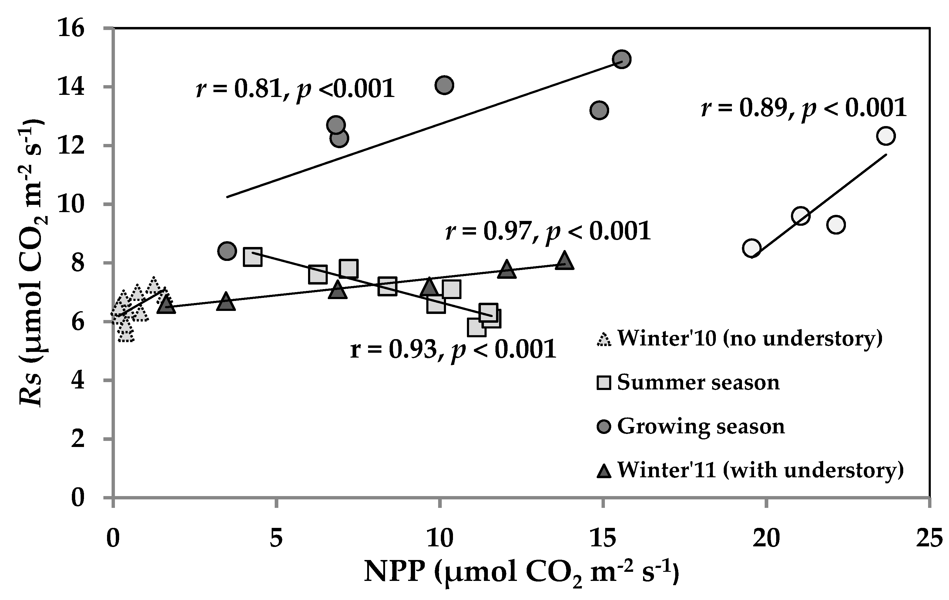
3.5. Temporal Correlation of NPP and Rs across the Seasons and Relation with LAI

To understand how photosynthetic carbon input and Rs were coupled seasonally in this deciduous pine forest, we analyzed their inter-linkage (Figure 5). Dynamics of temporal correlation between Rs and NPP (seasonal coupling and decoupling behavior) has been shown using a coherence analysis (Figure S4). The Rs–NPP relation was positively correlated (r > 0.81, p < 0.001) over the growing season. In the post-monsoon, the correlation coefficient (r) between Rs and NPP was highest (r = 0.89). However, it was weakest (r = 0.58, p < 0.01) during winter 2010 (no understory) and strongest (r = 0.97, p < 0.001) during the same time-period in 2011 (with an understory). Notably, the Rs–NPP relation became inverse (r = 0.93, p < 0.001) during two to three months of the water-limitation period in the summer or pre-monsoon.

A minimum NPP of 0.7 ± 0.14 (s.e.) μmol CO₂ m⁻² s⁻¹ was observed during winter 2010, while a maximum of 19.5 ± 2 μmol CO₂ m⁻² s⁻¹ was observed during the post-monsoon season. The LAI of pine showed a unimodal seasonal pattern that varied from 0.55 to 6.44 with a mean of 4.0 (s.d. = 2.21, s.e = 0.36). A peak in LAI was attained during the monsoon and maintained for at least three months (August to October). Declining LAI was observed after the setting of the winter season. The LAI–NPP was positively correlated (Figure 6) across the growing season (R² = 0.83, p < 0.001). The LAI–NPP was also positively correlated during summer period and winter 2011 (R² = 0.82, p < 0.001; with an understory), while no correlation during winter 2010 (without an understory). It can be noted that LAI dynamics was found to be the major and overall regulator of the productivity.

4. Discussion

4.1. Seasonal Variability of Ecosystem CO₂ Fluxes

Components of carbon balance, such as Ac (~GPP), Rs, and NPP exhibited a strong seasonality in this subtropical pine forest having an understory as lantana. Both Rs and NPP peaked during the post-monsoon season and were lowest in the winter, which is typical for any temperate or subtropical coniferous forests [5,32]. The daily minimum and maximum rates of NPP were well comparable with the existing literatures for any temperate and subtropical coniferous forests [5,33,34]. For instance, the NPP from mixed forest plantation was reported in the rage of 2 μmol CO₂ m⁻² s⁻¹ to 6 μmol CO₂ m⁻² s⁻¹ over Northern Himalaya [33,35]. Notably, we observed that the NPP was almost 11 times higher during winter 2011 owing to the presence of an understory as compared to winter 2010.

Soil respiration (Rs) is an integral part of the ecosystem carbon cycle and coupled to various components of ecosystem production and decomposition processes. Rs is directly related to ecosystem carbon balance, nutrient cycling, regional-global carbon cycling, and climate change. Moreover, it plays a critical role in regulating atmospheric CO₂ concentration and thus, climate dynamics. However, given its ecological significance and role in atmospheric CO₂ concentration, it is unknown how climate warming would affect the positive feedback loop between the global carbon cycle and climate system and what is its role of soil respiration in regulating this positive feedback. To understand these pertinent questions, we have tried to decipher the biotic and abiotic controls in a pine forest of lower Himalaya.

Soil respiration (Rs) and productivity (NPP) relations were prominent at a seasonal time-scale as evidenced by their tight-link during the growing period, while they decoupled during the summer-time water stress. Studies across a variety of biomes also revealed a strong correlation between Rs and NPP [36,37]. A tight-link between Rs and NPP was obvious because primary production provides the organic substrate that drives soil metabolic activities [38]. However, a complete reversal in the Rs–NPP relation was noticed (r = −0.93), when winter-time temperature-limited conditions changed to the water-limitation period during summer (April–June). It was probably due to a reduction in photosynthate availability (as the overstory and understory canopy was still developing) as well as moisture stress-induced reduction in soil metabolism. Anaplerotic uptake of CO₂ could be another reason. Emergence of new leaves and canopy development is an important phase in the annual phenological cycle. In this critical phase, in the absence of sufficient numbers of matured leaves, the central process in energy metabolism, i.e., the tricarboxylic acid (TCA) cycle, increasingly functions to biosynthesize essential, non-essential amino acids, fatty acids, glucose, etc. The anaplerotic uptake of CO₂ ensures continued function of TCA cycle even if anions are removed from the cycle for biosynthesis. Accordingly, during dark CO₂ fixation, an additional inorganic carbon is essential for amino acid synthesis during canopy development so, additional carbon can be sourced either through the scavenging of respired CO₂ or through the uptake of CO₂ from the surrounding atmosphere. It is reasonable to conclude that during summer, Rs decouples from photosynthetic carbon input and it reduces due to a combined effect of photosynthate availability and water deficit. Even during dormant winter, understory played a crucial role in determining the strength of the Rs–NPP relation.

The carbon source/sink of the pine forest across the seasons was illustrated in Table 2. The understory was cleared before the experimentation started in November 2010 and overstory pine was in winter dormancy due to which the system acted as a source of carbon (384 ± 0.9 g C m⁻² month⁻¹) and persisted until the advent of spring (March). During the growing season (May–July), the pine forest was a sink of carbon (–315 ± 5.4 g C m⁻² month⁻¹), but having a larger carbon sink in the post-monsoon season (–508 ± 23 g C m⁻² month⁻¹). A notable decline in NEE was observed (208 ± 8.6 g C m⁻² month⁻¹) during rainy and overcast days in the monsoon season (e.g., July3d–Aug3d). The year 2010–2011 received about 31% higher precipitation than the long-term average (i.e., 70 years). This decline in NEE was mostly because of the decline in canopy photosynthesis, while soil and foliage respiration remained enhanced and even it was at its peak. These findings were also consistent with Zhang et al. [39] that suggested clouds can significantly affect NEE in a temperate pine mixed forest and in a subtropical evergreen broad-leaved forest in China. Watham et al. [33] while working in this region in a young, mixed-deciduous broad-leaved forest at 300 m of elevation (mean rainfall of 1500 mm), they reported that the nine year old mixed forest plantation (comprising of Holoptelea integrifolia, Dalbergia sissoo, Acacia catechu, and Albizia procera) remained as a carbon sink in July–August during 2013. Thus, the number of rainy days and monsoon dry-wet spells may have a marked influence on NEE.

In particular, at the seasonal time-scale, NPP exceeded Rs almost during the growing season (April–October), and consequently NEE has exhibited a net carbon uptake. During the winter and spring seasons, NEE was consistently positive (or the carbon source) due to the physiological dormancy stage of pine forest. These results were consistent with the physiological understanding of ecosystems, and with other studies in the region in broadleaf young deciduous vegetation types [33] and forests worldwide [40]. Further, presence of lantana (an invasive understory) during winter 2011 had helped to drop down the magnitude of the carbon source. Nevertheless, at the annual time-scale, the system remained as a carbon sink (−99 ± 9.9 g C m⁻² year⁻¹). The magnitudes of the carbon sink were within the range of other studies that reported across the variety of ecosystems worldwide [41]. However, our estimated annual carbon sink was lower than the Pinus forests over Europe and North America that ranged from −224 g C m⁻² year⁻¹ to −277 g C m⁻² year⁻¹ [42,43].

4.2. Factors Affecting Ecosystem CO₂ Fluxes

Evaporative fraction-temperature explained maximum variability in the fluxes over this energy-limited ecosystem. Usually, temperature is the most important abiotic factor influencing biological systems across the scales from the biochemical kinetic reactions to ecosystem biogeochemical processes including carbon cycling. In particular, in the energy-limited ecosystems, as in this case of the Himalayan ecosystem, solar incoming radiation and temperature played a crucial role in photosynthesis and respiration. By looking into the significance of defining the temperature threshold points, we observed that the optimal temperature was 25 °C and NEE became positive when the temperature was below 10 °C. In relation to moisture availability, we observed that optimal EF that maximizes both NPP and NEE was observed between 0.5 and 0.75. Both NPP and NEE declined when EF exceeded 0.75 or dropped below 0.5. VPD between 0.6 kPa and 2.0 kPa was optimal for NPP and NEE. We also observed that Rs rates were mostly determined by abiotic factors such as soil/air temperature and EF. These observations were consistent with Wangdi et al. [44], which indicated that the temperatures and EF has a larger control on Rs flux. The seasonal pattern of Rs was consistent as reported from a central Himalayan region [32].

It is well established that under non-limiting light-moisture conditions, NPP is mainly governed by green leaf area in most forest ecosystems [45,46]. The NPP–LAI was found positively correlated across the growing season (R² = 0.83, p < 0.001). We observed that temperature played a key role in regulating NPP in a pine ecosystem and a similar conclusion was obtained in a southern boreal forest in Finland [47]. A decline in VPD led to an increase in NPP, with the exception during winter with declining LAI. A pronounced effect of VPD on NPP was consistent with the conclusions of Williams et al. [48] and Stella et al. [49] over pine forests from Northern America and Europe, respectively. Besides, these physical factors and anthropogenic interventions, phenological cycle (LAI) played an important role in determining the sink and source capacity of a deciduous pine ecosystem in western Himalaya.

4.3. Seasonal Variability of CUE and Associated Factors

The ecosystem CUE (ratio of NPP to GPP) is often used as an index of carbon flux efficiency from atmosphere to the vegetation, and to decipher the effects of forest management on carbon balance [31]. CUE is a critical ecosystem property for productivity models. The historical concept of “constant CUE” has been discarded, as it can vary with ecosystem-type, climate, nutrients, and locations [31,50,51]. Further, we showed that CUE is also dependent on the forest management practices (e.g., understory removal). The CUE has a large spatial-temporal variation (0.23–0.83) over forest ecosystems [31]. Our results underlined that CUE varied largely across the seasons (0.3 to 0.8) and mean growing season CUE was 0.74 ± 0.02 (s.e.). Annual CUE of this subtropical pine forests stands at 0.64 ± 0.03 (s.e.). A higher CUE in a warm-moist regime in this subtropical region with ~240 days of growing period can be theoretically expected. Zanotelli et al. [52] while working in a similar warm-moist environmental setup observed comparable CUE (0.71 ± 0.09). The mean CUE in the winter 2011 (with an understory) and in the winter 2010 (no understory) were 0.63 and 0.29, respectively. Typically, the forest management practice such as understory removal favors the growth of overstory (pine). By contrast, in view of carbon balance, this practice could lead to lower CUE. Consequently, it may lead to a release of carbon (positive NEE) from pine ecosystems over Himalaya.

4.4. Uncertainty Associated with CO₂ Ecosystem Fluxes

The strength of this paper lays in the analysis of the manual but numerous chamber-based flux measurements through systematic sampling in different quadrats, but it is also pertinent to mention here the possible source of uncertainty in the measurements of ecophysiological variables and chamber–based upscaling method. Lack of spatial representativeness is the most important source of systematic error in Rs measurements [53]. To obtain sufficient spatial representativeness of both the root and non-root zone with a single measurement system, these zones were hourly and alternatively sampled in different random quadrats. To supplement these measurements, periodic measurements were also carried out through another static-chamber IRGA-based instrument. Diffusion-leak may become a significant source of error in the chamber-based methodology. We carefully considered it every time while operating the photosynthesis system and ensured it by ‘valve matching’, as it was routinely performed every 30 min to maintain prevailing ambient conditions and to correct any analyzer offsets. Further, sufficient numbers (350–450) of systematic hourly readings minimized random error (coefficient of variation). The usual auto-correlation between ecosystem respiration (Re) and NEE was avoided in this study, which was hardly possible with the EC system without errors [54]. Nevertheless, systematic error of ~15–20% associated with chamber-based methodology was assumed in this study [53], especially when intended to measure individual carbon balance components [55,56,57].

We acknowledge that study on seasonal carbon balance behavior of a mature pine forest in the Himalaya is rare. However, studies on annual biomass based productivity estimates phytogeography, phenology are available [58]. It is suggested that Pinus roxburghii is not the potential natural climax forest but has been stabilized extensively and currently regarded as a permanent feature. Its extensive occurrence in the Himalaya has been attributed to continuing disturbances, such as deforestation, burning, and landslides. Mature forest attains a height of 30–35 m, whereas, canopy is open and crown density is below 60%. The understory shrub layer of a mature forest is poor, and grasses dominate because of frequent burning. However, in this study we found that the shrub layer was an important contributor to the ecosystem carbon balance. Thus, it appears that with the maturity of the forest, importance of shrub layer diminishes. Biomass and allometric equation based annual productivity estimates of Pinus roxburghii forest indicate a range of 7.6 ton ha⁻¹ year⁻¹ to 18.7 ton ha⁻¹ year⁻¹, which is similar to this study in young pines. Studies mainly focus on above ground and below ground productivity estimates remain controversial. The plant height and canopy spread at successive stages indicates saturation above the age of around 60 [58]. The total photosynthetic and non-photosynthetic biomass ratio also declines as the tree ages. An estimate indicates a five times more relative accumulation of biomass occurs in non-photosynthetic parts during the later years of growth. We found the ratio at 0.09 for this young pine and the reported ratio at the age of 25 years is 0.082. Accordingly, maximum increment in mature trees biomass occurs at the age around ~40 years. Still a knowledge gap exists between behaviors of young with that of mature trees. Therefore, the future research direction should focus on long-term monitoring of different components of ecosystem carbon balance, controlling climatic factors including disturbances.

5. Conclusions

Subtropical deciduous pine (chir pine) forests in western Himalaya regions are underrepresented in global assessments concerning forest carbon dynamics and productivity, and so far no comprehensive in situ data were available on carbon exchange dynamics from pine forests. This study revealed that pine forests with understory (lantana: An invasive species) have a large carbon uptake potential, particularly during the growing period, and thus, it can be concluded that subtropical pine forests are strong carbon sinks during favorable environmental conditions. In the post-monsoon season, the highest strong carbon sink was noticed, while a reduction in incoming solar radiation (reduced PAR) due to cloudiness could lead to transient phase reversal in this energy-limited pine ecosystem. Furthermore, carbon dynamics in this ecosystem were strongly controlled by temperature, EF, and VPD other than LAI and PAR. Removal of the understory is a prevalent forest management practice in the Himalaya, but this practice may not be a viable option for gaining and maintaining carbon balance in pine forests over the Himalaya. The understory (lantana) is extensively distributed in the Himalaya, and it turned out to be a significant component of the forest carbon balance. This can be attributed to sustained NPP from the understory during the lean season (November–February). On the contrary, lantana (known as an invasive detrimental weed) could pose serious problems in plantation forestry. It can obstruct overstory vegetation and become the dominant species causing a threat to the native flora. Moreover, long-term time-series data are essential to assess the degree of inter-annual variability of carbon dynamics in response to environmental conditions and climate. Nonetheless, these findings may be useful in understanding the carbon balance over a relatively understudied region of the world.

References

1. Le Quéré, C.; Andres, R.J.; Boden, T.; Conway, T.; Houghton, R.A.; House, J.I.; Marland, G.; Peters, G.P.; van der Werf, G.R.; Ahlström, A.; et al. The global carbon budget 1959–2011. Earth Syst. Sci. Data 2013, 5, 165–185. [Google Scholar] [CrossRef] [Green Version]
2. Sitch, S.; Friedlingstein, P.; Gruber, N.; Jones, S.D.; Murray-Tortarolo, G.; Ahlström, A.; Doney, S.C.; Graven, H.; Heinze, C.; Huntingford, C.; et al. Recent trends and drivers of regional sources and sinks of carbon dioxide. Biogeosciences 2015, 12, 653–679. [Google Scholar] [CrossRef] [Green Version]
3. Pan, Y.; Birdsey, R.A.; Fang, J.; Houghton, R.; Kauppi, P.E.; Kurz, W.A.; Phillips, O.L.; Shvidenko, A.; Lewis, S.L.; Canadell, J.G.; et al. A Large and Persistent Carbon Sink in the World’s Forests. Science 2011, 333, 988–993. [Google Scholar] [CrossRef] [PubMed]
4. Ahlstrom, A.; Raupach, M.R.; Schurgers, G.; Smith, B.; Arneth, A.; Jung, M.; Reichstein, M.; Canadell, J.G.; Friedlingstein, P.; Jain, A.K.; et al. The dominant role of semi-arid ecosystems in the trend and variability of the land CO2 sink. Science 2015, 348, 895–899. [Google Scholar] [CrossRef] [PubMed]
5. Baldocchi, D. “Breathing” of the terrestrial biosphere: lessons learned from a global network of carbon dioxide flux measurement systems. Aust. J. Bot. 2008, 56, 1. [Google Scholar]
6. Beringer, J.; Hutley, L.B.; McHugh, I.; Arndt, S.K.; Campbell, D.; Cleugh, H.A.; Cleverly, J.; Resco de Dios, V.; Eamus, D.; Evans, B.; et al. An introduction to the Australian and New Zealand flux tower network–OzFlux. Biogeosciences 2016, 13, 5895–5916. [Google Scholar] [CrossRef]
7. Singh, N.; Parida, B.R. Environmental factors associated with seasonal variations of night-time plant canopy and soil respiration fluxes in deciduous conifer forest, Western Himalaya, India. Trees 2019, 33, 599–613. [Google Scholar] [CrossRef]
8. Keenan, T.F.; Migliavacca, M.; Papale, D.; Baldocchi, D.; Reichstein, M.; Torn, M.; Wutzler, T. Widespread inhibition of daytime ecosystem respiration. Nat. Ecol. Evol. 2019, 3, 407–415. [Google Scholar] [CrossRef]
9. Basistha, A.; Arya, D.S.; Goel, N.K. Analysis of historical changes in rainfall in the Indian Himalayas. Int. J. Climatol. 2009, 29, 555–572. [Google Scholar] [CrossRef] [Green Version]
10. Shrestha, U.B.; Gautam, S.; Bawa, K.S. Widespread Climate Change in the Himalayas and Associated Changes in Local Ecosystems. PLoS ONE 2012, 7, e36741. [Google Scholar] [CrossRef] [Green Version]
11. Forest Survey of India. Indian State of Forest Report 2011; Ministry of Environment and Forests: Dehradun, India, 2011.
12. Singh, N.; Bhattacharya, B.K.; Nanda, M.K.; Soni, P.; Parihar, J.S. Radiation and energy balance dynamics over young chir pine (Pinus roxburghii) system in Doon of western Himalayas. J. Earth Syst. Sci. 2014, 123, 1451–1465. [Google Scholar] [CrossRef]
13. Singh, N.; Patel, N.R.; Bhattacharya, B.K.; Soni, P.; Parida, B.R.; Parihar, J.S. Analyzing the dynamics and inter-linkages of carbon and water fluxes in subtropical pine (Pinus roxburghii) ecosystem. Agric. For. Meteorol. 2014, 197, 206–218. [Google Scholar] [CrossRef]
14. Speckman, H.N.; Frank, J.M.; Bradford, J.B.; Miles, B.L.; Massman, W.J.; Parton, W.J.; Ryan, M.G. Forest ecosystem respiration estimated from eddy covariance and chamber measurements under high turbulence and substantial tree mortality from bark beetles. Glob. Change Biol. 2015, 21, 708–721. [Google Scholar] [CrossRef]
15. Hill, T.; Chocholek, M.; Clement, R. The case for increasing the statistical power of eddy covariance ecosystem studies: Why, where and how? Glob. Change Biol. 2017, 23, 2154–2165. [Google Scholar] [CrossRef]
16. Berkelhammer, M.; Hu, J.; Bailey, A.; Noone, D.C.; Still, C.J.; Barnard, H.; Gochis, D.; Hsiao, G.S.; Rahn, T.; Turnipseed, A. The nocturnal water cycle in an open-canopy forest. J. Geophys. Res. Atmos. 2013, 118, 10225–10242. [Google Scholar] [CrossRef]
17. Collier, S.M.; Ruark, M.D.; Oates, L.G.; Jokela, W.E.; Dell, C.J. Measurement of Greenhouse Gas Flux from Agricultural Soils Using Static Chambers. J. Vis. Exp. 2014. [Google Scholar] [CrossRef] [PubMed] [Green Version]
18. Law, B.E.; Kelliher, F.M.; Baldocchi, D.D.; Anthoni, P.M.; Irvine, J.; Moore, D.; Van Tuyl, S. Spatial and temporal variation in respiration in a young ponderosa pine forest during a summer drought. Agric. For. Meteorol. 2001, 110, 27–43. [Google Scholar] [CrossRef]
19. Cavaleri, M.A.; Oberbauer, S.F.; Ryan, M.G. Foliar and ecosystem respiration in an old-growth tropical rain forest. Plant Cell Environ. 2008, 31, 473–483. [Google Scholar] [CrossRef] [PubMed] [Green Version]
20. Chambers, J.Q.; Tribuzy, E.S.; Toledo, L.C.; Crispim, B.F.; Higuchi, N.; dos Santos, J.; Araújo, A.C.; Kruijt, B.; Nobre, A.D.; Trumbore, S.E. Respiration from a Tropical Forest Ecosystem: Partitioning of sources and low Carbon Use Efficiency. Ecol. Appl. 2004, 14, 72–88. [Google Scholar] [CrossRef]
21. Campbell, G.; Norman, J. An Introduction to Environmental Biophysics; Springer-Verlag New York: New York, NY, USA, 1998; p. 71. [Google Scholar]
22. Sun, J.; Guan, D.; Wu, J.; Jing, Y.; Yuan, F.; Wang, A.; Jin, C. Day and night respiration of three tree species in a temperate forest of northeastern China. IForest 2015, 8, 25–32. [Google Scholar] [CrossRef] [Green Version]
23. Wehr, R.; Munger, J.W.; McManus, J.B.; Nelson, D.D.; Zahniser, M.S.; Davidson, E.A.; Wofsy, S.C.; Saleska, S.R. Seasonality of temperate forest photosynthesis and daytime respiration. Nature 2016, 534, 680–683. [Google Scholar] [CrossRef]
24. Amthor, J.S.; Baldocchi, D.D. Terrestrial higher plant respiration and net primary productivity. In Terrestrial Global Productivity; Roy, J., Mooney, H., Saugier, B., Eds.; Elsevier: New York, NY, USA, 2001; pp. 33–59. [Google Scholar]
25. Allison, S.D.; Wallenstein, M.D.; Bradford, M.A. Soil-carbon response to warming dependent on microbial physiology. Nat. Geosci. 2010, 3, 336–340. [Google Scholar] [CrossRef]
26. Leuning, R.; van Gorsel, E.; Massman, W.J.; Isaac, P.R. Reflections on the surface energy imbalance problem. Agric. For. Meteorol. 2012, 156, 65–74. [Google Scholar] [CrossRef]
27. Heusinkveld, B.G.; Jacobs, A.F.G.; Holtslag, A.A.M.; Berkowicz, S.M. Surface energy balance closure in an arid region: Role of soil heat flux. Agric. For. Meteorol. 2004, 122, 21–37. [Google Scholar] [CrossRef]
28. Seneviratne, S.I.; Corti, T.; Davin, E.L.; Hirschi, M.; Jaeger, E.B.; Lehner, I.; Orlowsky, B.; Teuling, A.J. Investigating soil moisture–climate interactions in a changing climate: A review. Earth-Sci. Rev. 2010, 99, 125–161. [Google Scholar] [CrossRef]
29. Grinsted, A.; Moore, J.C.; Jevrejeva, S. Application of the cross wavelet transform and wavelet coherence to geophysical time series. Nonlinear Process. Geophys. 2004, 11, 561–566. [Google Scholar] [CrossRef] [Green Version]
30. Torrence, C.; Compo, G.P. A Practical Guide to Wavelet Analysis. Bull. Am. Meteorol. Soc. 1998, 79, 61–78. [Google Scholar] [CrossRef] [Green Version]
31. DeLUCIA, E.H.; Drake, J.E.; Thomas, R.B.; Gonzalez-Meler, M. Forest carbon use efficiency: Is respiration a constant fraction of gross primary production? Glob. Change Biol. 2007, 13, 1157–1167. [Google Scholar] [CrossRef]
32. Joshi, M.; Mer, G.S.; Singh, S.P.; Rawat, Y.S. Seasonal pattern of total soil respiration in undisturbed and disturbed ecosystems of Central Himalaya. Biol. Fertil. Soils 1991, 11, 267–272. [Google Scholar] [CrossRef]
33. Watham, T.; Kushwaha, S.P.; Patel, N.R.; Dadhwal, V.K. Monitoring of carbon dioxide and water vapour exchange over a young mixed forest plantation using eddy covariance technique. Curr. Sci 2014, 107, 858–867. [Google Scholar]
34. Singh, N.; Patel, N.R.; Singh, J.; Raja, P.; Soni, P.; Parihar, J.S. Carbon exchange in some invasive species in the Himalayan foothills. Trop. Ecol. 2016, 57, 263–270. [Google Scholar]
35. Patel, N.R.; Padalia, H.; Kushwaha, S.P.S.; Nandy, S.; Watham, T.; Ahongshangbam, J.; Kumar, R.; Dadhwal, V.K.; Senthil, K.A. CO2 Flux Tower and Remote Sensing: Tools for Monitoring Carbon Exchange over Ecosystem Scale in Northwest Himalaya; Navalgund, R., Kumar, A., Nandy, S., Eds.; Springer: Singapore, 2019. [Google Scholar]
36. Bahn, M.; Rodeghiero, M.; Anderson-Dunn, M.; Dore, S.; Gimeno, C.; Drösler, M.; Williams, M.; Ammann, C.; Berninger, F.; Flechard, C.; et al. Soil Respiration in European Grasslands in Relation to Climate and Assimilate Supply. Ecosystems 2008, 11, 1352–1367. [Google Scholar] [CrossRef] [Green Version]
37. DeForest, J.L.; Noormets, A.; McNulty, S.G.; Sun, G.; Tenney, G.; Chen, J. Phenophases alter the soil respiration–temperature relationship in an oak-dominated forest. Int. J. Biometeorol. 2006, 51, 135–144. [Google Scholar] [CrossRef] [PubMed]
38. Yuan, W.; Luo, Y.; Li, X.; Liu, S.; Yu, G.; Zhou, T.; Bahn, M.; Black, A.; Desai, A.R.; Cescatti, A.; et al. Redefinition and global estimation of basal ecosystem respiration rate. Glob. Biogeochem. Cycles 2011, 25, 1–14. [Google Scholar] [CrossRef]
39. Zhang, M.; Yu, G.-R.; Zhang, L.-M.; Sun, X.-M.; Wen, X.-F.; Han, S.-J.; Yan, J.-H. Impact of cloudiness on net ecosystem exchange of carbon dioxide in different types of forest ecosystems in China. Biogeosciences 2010, 7, 711–722. [Google Scholar] [CrossRef] [Green Version]
40. Canadell, J.G.; Mooney, H.A.; Baldocchi, D.D.; Berry, J.A.; Ehleringer, J.R.; Field, C.B.; Gower, S.T.; Hollinger, D.Y.; Hunt, J.E.; Jackson, R.B.; et al. Commentary: Carbon Metabolism of the Terrestrial Biosphere: A Multitechnique Approach for Improved Understanding. Ecosystems 2000, 3, 115–130. [Google Scholar] [CrossRef] [Green Version]
41. Xue, B.-L.; Guo, Q.; Gong, Y.; Hu, T.; Liu, J.; Ohta, T. The influence of meteorology and phenology on net ecosystem exchange in an eastern Siberian boreal larch forest. J. Plant Ecol. 2016, 9, 520–530. [Google Scholar] [CrossRef] [Green Version]
42. Suni, T.; Berninger, F.; Markkanen, T.; Keronen, P.; Rannik, Ü.; Vesala, T. Interannual variability and timing of growing-season CO2 exchange in a boreal forest. J. Geophys. Res. Atmos. 2003, 108. [Google Scholar] [CrossRef]
43. McCaughey, J.H.; Lafleur, P.M.; Joiner, D.W.; Bartlett, P.A.; Costello, A.M.; Jelinski, D.E.; Ryan, M.G. Magnitudes and seasonal patterns of energy, water, and carbon exchanges at a boreal young jack pine forest in the BOREAS northern study area. J. Geophys. Res. Atmos. 1997, 102, 28997–29007. [Google Scholar] [CrossRef] [Green Version]
44. Wangdi, N.; Mayer, M.; Nirola, M.P.; Zangmo, N.; Orong, K.; Ahmed, I.U.; Darabant, A.; Jandl, R.; Gratzer, G.; Schindlbacher, A. Soil CO2 efflux from two mountain forests in the eastern Himalayas, Bhutan: Components and controls. Biogeosciences 2017, 14, 99–110. [Google Scholar] [CrossRef]
45. Lindroth, A.; Verwijst, T.; Halldin, S. Water-use efficiency of willow: Variation with season, humidity and biomass allocation. J. Hydrol. 1994, 156, 1–19. [Google Scholar] [CrossRef]
46. Alton, P.B.; North, P.R.; Los, S.O. The impact of diffuse sunlight on canopy light-use efficiency, gross photosynthetic product and net ecosystem exchange in three forest biomes: Impact of Diffuse Sunlight on canopy LUE, GPP and NEE. Glob. Change Biol. 2007, 13, 776–787. [Google Scholar] [CrossRef]
47. Kolari, P.; Lappalainen, H.K.; HäNninen, H.; Hari, P. Relationship between temperature and the seasonal course of photosynthesis in Scots pine at northern timberline and in southern boreal zone. Tellus B Chem. Phys. Meteorol. 2007, 59, 542–552. [Google Scholar] [CrossRef] [Green Version]
48. Williams, M.; Law, B.E.; Anthoni, P.M.; Unsworth, M.H. Use of a simulation model and ecosystem flux data to examine carbon-water interactions in ponderosa pine. Tree Physiol. 2001, 21, 287–298. [Google Scholar] [CrossRef] [PubMed] [Green Version]
49. Stella, P.; Lamaud, E.; Brunet, Y.; Bonnefond, J.-M.; Loustau, D.; Irvine, M. Simultaneous measurements of CO2 and water exchanges over three agroecosystems in South-West France. Biogeosciences 2009, 6, 2957–2971. [Google Scholar] [CrossRef]
50. Lambers, H. Cyanide-resistant respiration: A non-phosphorylating electron transport pathway acting as an energy overflow. Physiol. Plant. 1982, 55, 478–485. [Google Scholar] [CrossRef]
51. Vicca, S.; Luyssaert, S.; Peñuelas, J.; Campioli, M.; Chapin, F.S.; Ciais, P.; Heinemeyer, A.; Högberg, P.; Kutsch, W.L.; Law, B.E.; et al. Fertile forests produce biomass more efficiently: Forests’ biomass production efficiency. Ecol. Lett. 2012, 15, 520–526. [Google Scholar] [CrossRef] [PubMed]
52. Zanotelli, D.; Montagnani, L.; Manca, G.; Tagliavini, M. Net primary productivity, allocation pattern and carbon use efficiency in an apple orchard assessed by integrating eddy covariance, biometric and continuous soil chamber measurements. Biogeosciences 2013, 10, 3089–3108. [Google Scholar] [CrossRef] [Green Version]
53. Luo, Y.; Zhou, X. Soil Respiration and the Environment; Academic Press: San Diego, CA, USA, 2010; pp. 1–328. ISBN 9780120887828. [Google Scholar]
54. Baldocchi, D.; Sturtevant, C.; Contributors, F. Does day and night sampling reduce spurious correlation between canopy photosynthesis and ecosystem respiration? Agric. For. Meteorol. 2015, 207, 117–126. [Google Scholar] [CrossRef] [Green Version]
55. Lee, X.; Massman, W.; Law, B.E. Handbook of Micrometeorology: A Guide for Surface Flux Measurement and Analysis; Kluwer Academic Publishers: Dordrecht, The Netherlands, 2004; ISBN 1-402022646. [Google Scholar]
56. Aubinet, M.; Feigenwinter, C.; Heinesch, B.; Bernhofer, C.; Canepa, E.; Lindroth, A.; Montagnani, L.; Rebmann, C.; Sedlak, P.; Van Gorsel, E. Direct advection measurements do not help to solve the night-time CO2 closure problem: Evidence from three different forests. Agric. For. Meteorol. 2010, 150, 655–664. [Google Scholar] [CrossRef]
57. Billesbach, D.P. Estimating uncertainties in individual eddy covariance flux measurements: A comparison of methods and a proposed new method. Agric. For. Meteorol. 2011, 151, 394–405. [Google Scholar] [CrossRef]
58. Singh, J.S. Forests of Himalaya: Structure, Functioning and Impact of Man; Gyanodaya Prakashan: Nainital, India, 1992; pp. 1–294. [Google Scholar]
Figure 1. Variations of carbon fluxes net primary productivity (NPP), soil respiration (Rs), and net ecosystem carbon exchange (NEE; μmol CO2 m−2 s−1) at a 10-day (Dekads) interval over the period November 2010 to December 2011 (vertical bars as SE). Fluxes of the winter season 2010 and 2011 were without understory and with understory, respectively. Fluxes since April 2011 were aggregated of overstory and understory. NEE with a negative sign indicated a carbon sink.
Resources 08 00098 g001
Figure 2. Relationship between evaporative fraction (EF) and NPP at a 10-day (Dekads) interval over the growing period April to October 2011 (a). Solid circles indicate the growing period (April–June), while open circles indicate the peak growing period (July–September). In subplot (b), the relationship between the vapor pressure deficit (VPD) and NPP over the growing period April to October 2011 (solid circles) was shown (excluding August).
Resources 08 00098 g002
Figure 3. Variations of carbon use efficiency (CUE; ratios of NPP–Ac) in relation to the day-time air temperature (AT) at a 10-day (Dekads) interval over the period November 2010 to December 2011. The period November 2010 to March 2011 has no understory, while the rest of the period was with an understory.
Resources 08 00098 g003
Figure 4. The relationship between CUE and EF across the growing season was shown. Solid circles indicate the growing season (April–June), while open circles indicate the peak growing season (July–October) (a). October data were not included in the linear regression as the EF values (0.46 to 0.60) had a different cluster. In subplot (b), the relationship between CUE and VPD was shown.
Resources 08 00098 g004
Figure 5. Relationship between the Rs and net primary productivity (NPP) at a 10-day (Dekads) interval over the period November 2010 to December 2011. Solid circles indicate the growing period from (July3d–Sep2d), while open circles indicate the growing period from (Sept3d–Oct3d). Dotted open Δ denotes winter 2010 (no understory), but solid Δ denotes winter 2011 (with an understory). Solid □ indicates data pooled over the summer season (April–May) and pre-monsoon (June).
Resources 08 00098 g005
Figure 6. Relationship between leaf area index (LAI) and NPP at a 10-day (Dekads) interval over the period November 2010 to December 2011. In winter 2010 (no understory), no correlation was obtained. The legend used is as per Figure 5.
Resources 08 00098 g006