Evaluating the Response of Mediterranean-Atlantic Saltmarshes to Sea-Level Rise


Abstract
:1. Introduction
2. Materials and Methods
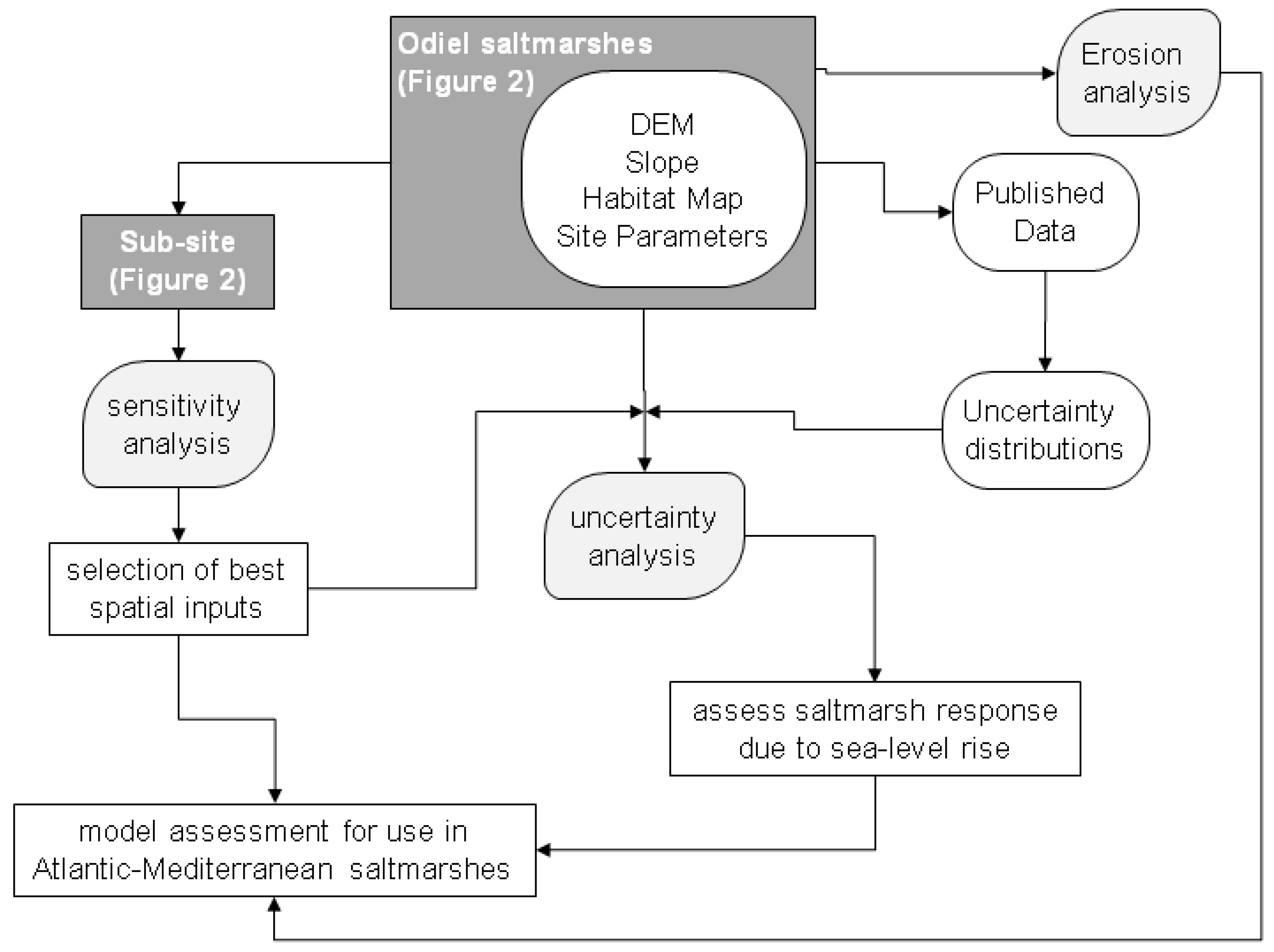
2.1. Research Design
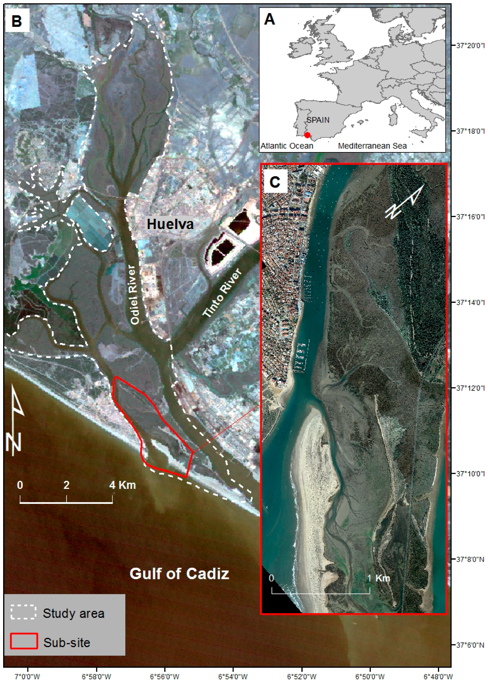
2.2. Study Area
2.3. SLAMM Model
2.4. Sensitivity Analysis of Spatial Model Inputs
2.5. Uncertainty Analysis
- Define the input uncertainty distributions
- Decide how many simulations lead to results which are robust (i.e., not seed sensitive) and accurate.
- Automatically generate random input values consistent with the uncertainty distributions.
- Run SLAMM multiple times with these pseudorandom inputs to evaluate how SLAMM outputs are affected (full calculation).
- Analyze the distribution of the model output outcomes to see if there are any common patterns helping the user to understand the dynamics/interaction of the previously defined uncertainty distributions of the model inputs.
2.6. Erosion Rates
3. Results
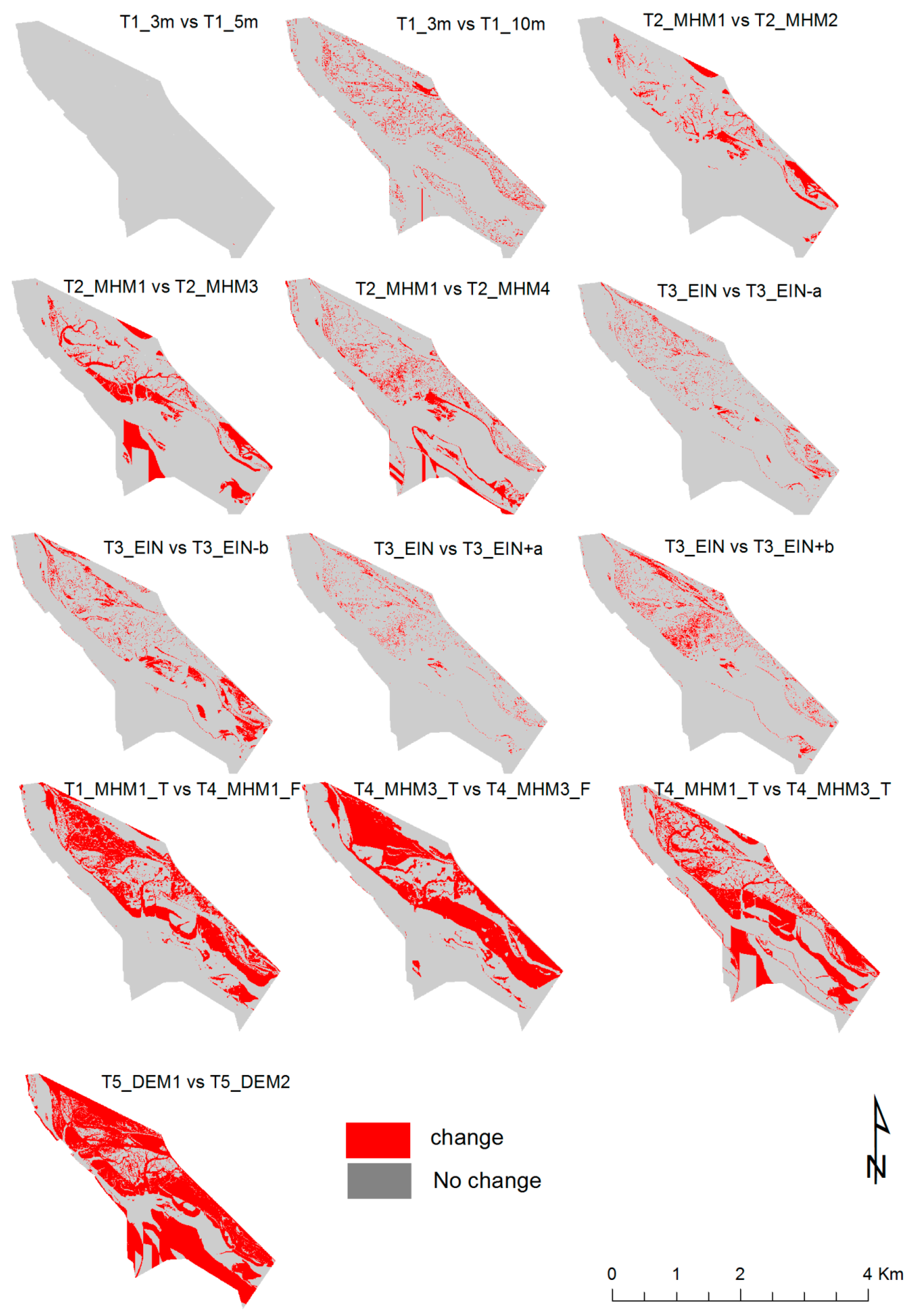
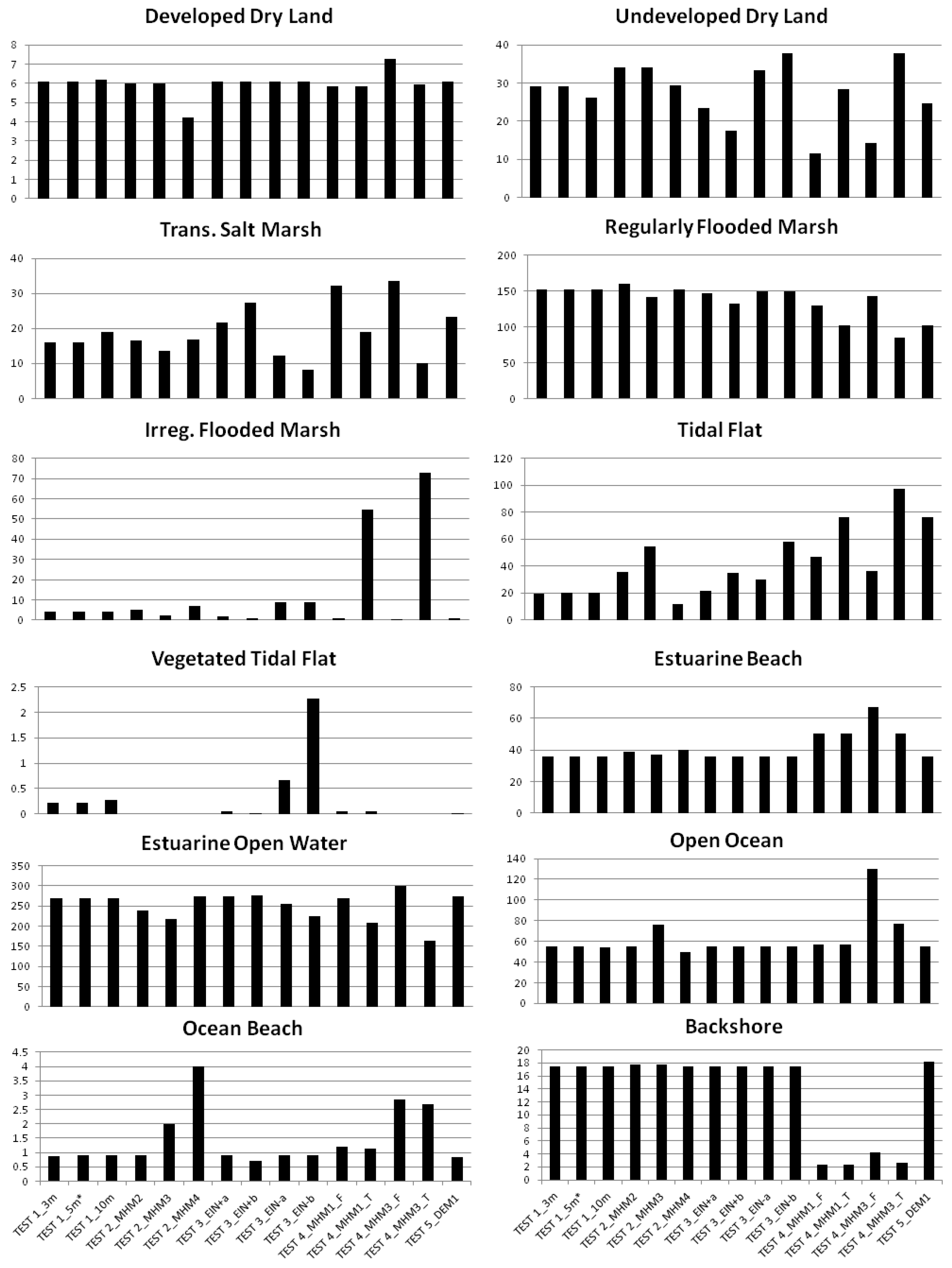
3.1. Sensitivity Analysis Based on Spatial Inputs
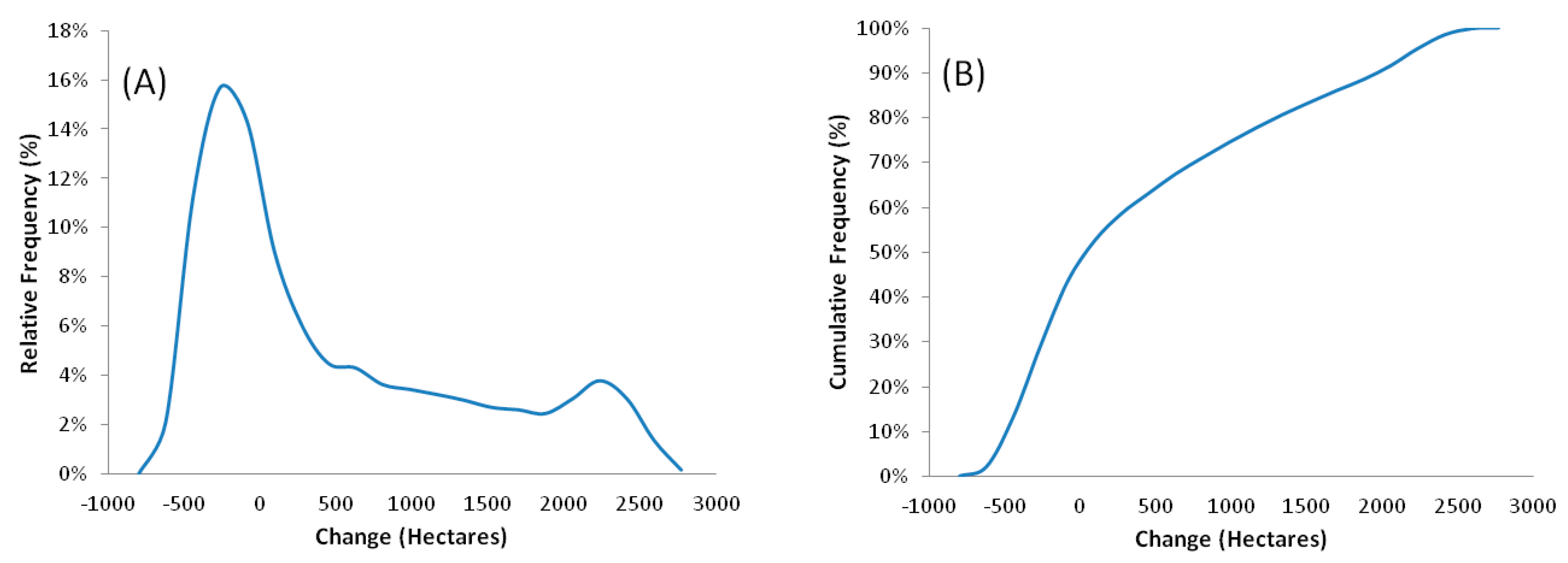
3.2. Uncertainty Analysis
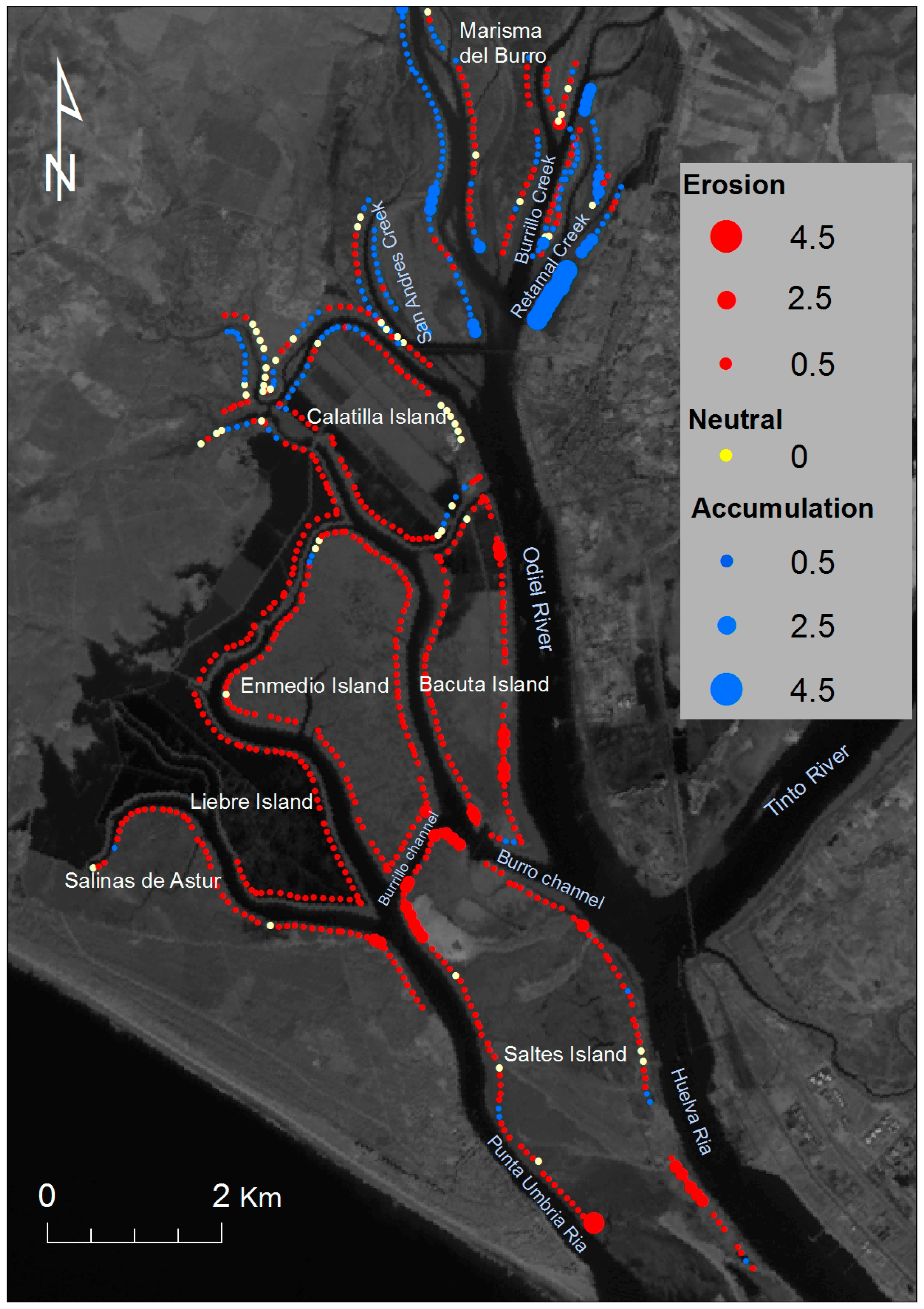
3.3. Assessment of the Erosion Rates
4. Discussion and Conclusions
Author Contributions
Funding
Conflicts of Interest
References
- Smith, S.M. Multi-Decadal Changes in Salt Marshes of Cape Cod, MA: Photographic Analyses of Vegetation Loss, Species Shifts, and Geomorphic Change. Northeast. Nat. 2009, 16, 183–208. [Google Scholar] [CrossRef]
- Nicholls, R.J. Coastal flooding and wetland loss in the 21st century: Changes under the SRES climate and socio-economic scenarios. Glob. Environ. Chang. 2004, 14, 69–86. [Google Scholar] [CrossRef]
- IPCC (Intergovernmental Panel on Climate Change). Climate Change 2014: Synthesis Report. Contribution of Working Groups I, II and III to the Fifth Assessment Report of the Intergovernmental Panel on Climate Change; Pachauri, R.K., Meyer, L.A., Eds.; IPCC: Geneva, Switzerland, 2014; p. 151. [Google Scholar]
- Pfeffer, W.T.; Harper, J.T.; O’Neel, S. Kinematic constraints on glacier contributions to 21st-century sea-level rise. Science 2008. [Google Scholar] [CrossRef] [PubMed]
- Rahmstorf, S. A semi-empirical approach to projecting future sea-level rise. Science 2007, 315, 368–370. [Google Scholar] [CrossRef]
- Meehl, G.A.; Stocker, T.S.; Collins, W.D.; Friedlingstein, P.; Gaye, A.T.; Gregory, J.M.; Kitoh, A.; Knutti, R.; Murhy, J.M.; Nosa, A.; et al. (Eds.) Contribution of Working Group I to the Fourth Assessment Report of IPCC on Climatic Change; Cambridge University Press: Cambridge, UK, 2007; pp. 749–844. [Google Scholar]
- Church, J.A.; Clark, P.U.; Cazenave, A.; Gregory, J.M.; Jevrejeva, S.; Levermann, A.; Merrifield, M.A.; Milne, G.A.; Nerem, R.S.; Nunn, P.D.; et al. Sea level change. In Climate Change, 2013: The Physical Science Basis; Stocker, T.F., Qin, D., Plattner, G.-K., Tignor, M., Allen, S.K., Boschung, J., Nauels, A., Xia, Y., Bex, V., Midgley, P.M., Eds.; Contribution of Working Group I to the Fifth Assessment Report of the Intergovernmental Panel on Climate Change; Cambridge University Press: Cambridge, UK; New York, NY, USA, 2013. [Google Scholar]
- Vermeer, M.; Rahmstorf, S. Global sea level linked to global temperature. Proc. Natl. Acad. Sci. USA 2009, 106, 21527–21532. [Google Scholar] [CrossRef] [PubMed] [Green Version]
- Jevrejeva, S.; Moore, J.C.; Grinsted, A. Sea level projections to AD2500 with a new generation of climate change scenarios. Glob. Planet Chang. 2012, 80–81, 14–20. [Google Scholar] [CrossRef]
- DeConto, R.M.; Pollard, D. Contribution of Antarctica to past and future sea-level rise. Nature 2016, 531, 591–597. [Google Scholar] [CrossRef] [PubMed]
- Oppenheimer, M.; Alley, R.B. How high will the seas rise? Science 2016, 354, 1375–1377. [Google Scholar] [CrossRef]
- Pugh, D.T. Tides, Surges and Mean Sea-Level; John Wiley & Sons Ltd.: New York, NY, USA, 1996. [Google Scholar]
- Rybczyk, J.M.; Callaway, C. Surface Elevation Models. In Coastal Wetlands: An Intergrated Ecosystem Approach; Perillo, G.M.E., Wolanski, E., Cahoon, D.R., Brinson, M.M., Eds.; Elsevier: Amsterdam, The Netherland, 2009; pp. 835–853. [Google Scholar]
- French, J. Tidal marsh sedimentation and resilience to environmental change: Exploratory modelling of tidal, sea-level and sediment supply forcing in predominantly allochthonous systems. Mar. Geol. 2006, 235, 119–136. [Google Scholar] [CrossRef]
- Barbier, E.B. Valuing Ecosystem Services for Coastal Wetland Protection and Restoration: Progress and Challenges. Resources 2013, 2, 213–230. [Google Scholar] [CrossRef] [Green Version]
- Hartig, E.K.; Gornitz, V.; Kolker, A.; Mushacke, F.; Fallon, D. Anthropogenic and climate-change impacts on salt marshes of Jamaica Bay, New York City. Wetlands 2002, 22, 71–89. [Google Scholar] [CrossRef]
- Luo, S.; Shao, D.; Long, W.; Liu, Y.; Sun, T.; Cui, B. Assessing ‘coastal squeeze’ of wetlands at the Yellow River Delta in China: A case study. Ocean Coast. Manag. 2018, 153, 193–202. [Google Scholar] [CrossRef]
- Park, R.A.; Manjit, S.T.; Mauseland, P.W.; Howe, R.C. The Effects of Sea Level Rise on US Coastal Wetlands. The Potential Effects of Global Climate Change on the United States: Appendix B-Sea Level Rise; U.S. Environmental Protection Agency: Washington, DC, USA, 1989.
- Clough, J.; Polaczyk, A.; Propato, M. Modeling the potential effects of sea-level rise on the coast of New York: Integrating mechanistic accretion and stochastic uncertainty. Environ. Model. Softw. 2016, 84, 349–362. [Google Scholar] [CrossRef] [Green Version]
- Hauer, M.E.; Evans, J.M.; Alexander, C.R. Sea-level rise and sub-county population projections in coastal Georgia. Popul. Environ. 2015, 37, 44–62. [Google Scholar] [CrossRef]
- Linhoss, A.C.; Kiker, G.A.; Aiello-Lammensc, M.A.; Chu-Agor, L.; Convertino, M.; Muñoz-Carpena, R.; Fischere, R.; Linkov, I. Decision analysis for species preservation under sea-level rise. Ecol. Model. 2013, 263, 264–272. [Google Scholar] [CrossRef] [Green Version]
- Murdukhayeva, A.; August, P.; Bradley, M.; LaBash, C.; Shaw, N. Assessment of Inundation Risk from Sea Level Rise and Storm Surge in Northeastern Coastal National Parks. J. Coast. Res. 2013, 29, 1–16. [Google Scholar] [CrossRef]
- Sherwood, E.T.; Greening, S. Potential impacts and management implications of climate change on Tampa Bay estuary critical coastal habitats. Environ. Manag. 2014, 53, 401–415. [Google Scholar] [CrossRef]
- Cole Ekberg, M.L.; Raposa, K.B.; Ferguson, W.F.; Ruddock, K.; Burke Watson, E. Development and Application of a Method to Identify Salt Marsh Vulnerability to Sea Level Rise. Estuar. Coast. 2017, 40, 694–710. [Google Scholar] [CrossRef]
- Gehu, J.M.; Rivas-Martinez, S. Classification of European salt plant communities. In Salt Marsh in Europe; Dijkema, K.S., Ed.; Council of Europe: Strasbourg, France, 1984; pp. 34–40. [Google Scholar]
- Orson, R.; Panageotou, W.; Leatherman, S.P. Response of tidal salt marshes of the US Atlantic and Gulf coasts to rising sea levels. J. Coast. Res. 1985, 1, 29–37. [Google Scholar] [CrossRef]
- Ojeda, J. Las Costas Andaluzas. In Geografía de Andalucía; López, A., Ed.; Ariel: Sevilla, España, 2003; pp. 118–135. [Google Scholar]
- Arnaud-Fassetta, G.; Bertrand, F.; Costa, S.; Davidsonc, R. The western lagoon marshes of the Ria Formosa (Southern Portugal): Sediment-vegetation dynamics, long-term to short-term changes and perspective. Cont. Shelf Res. 2006, 26, 363–384. [Google Scholar] [CrossRef]
- Clough, J.S.; Park, R.A.; Fuller, J. SLAMM 6 Beta Technical Documentation SLAMM 6 Technical Documentation. 2010; p. 51. Available online: http://warrenpinnacle.com/prof/SLAMM6/SLAMM6_Technical_Documentation.pdf (accessed on 8 March 2019).
- Fernandez-Nunez, M.; Burningham, H.; Ojeda, J. Improving accuracy of LiDAR-derived digital terrain models for saltmarsh management. J. Coast. Conserv. 2017, 21, 209–222. [Google Scholar] [CrossRef] [Green Version]
- Fernandez-Nunez, M. Fusion of Airborne LiDAR, Multispectral Imagery and Spatial Modelling for Understanding Saltmarsh Response to Sea-Level Rise. Ph.D. Thesis, University College London, London, UK, February 2017. [Google Scholar]
- Rubio, J.C.; Figueroa, M.E. Medio Físico, Vegetación de las Marismas de los ríos Odiel y Tinto (Huelva). Estudios Territoriales 1983, 9, 59–86. [Google Scholar]
- Chu-Agor, M.L.; Muñoz-Carpena, R.; Kiker, G.; Emanuelsson, A.; Linkov, I. Exploring vulnerability of coastal habitats to sea level rise through global sensitivity and uncertainty analyses. Environ. Model. Softw. 2011, 26, 596–604. [Google Scholar] [CrossRef]
- Permanent Service for Mean Sea Level (PSMSL). Available online: https://www.psmsl.org/ (accessed on 16 June 2018).
- Morales, J.A.; Gutiérrez de San Miguel, E.; Borrego, J.E. Tasas de sedimentation reciente en la Ria de Huelva. Geogaceta 2003, 33, 15–18. [Google Scholar]
- Sobol, I.M. Sensitivity estimates for non-linear mathematical models. Math. Model. Comput. Exp. 1993, 4, 407–414. [Google Scholar]
- Pajak, M.J.; Leatherman, S.P. The High Water Line as Shoreline Indicator. J. Coast. Res. 2002, 18, 329–337. [Google Scholar]
- Himmelstoss, E.A. Dsas 4.0. Instructions Installation Guide User. In Digital Shoreline Analysis System (DSAS) Version 4.0—An ArcGIS Extension for Calculating Shoreline Change: U.S. Geological Survey Open-File Report 2008-1278; Thieler, E.R., Himmelstoss, E.A., Zichichi, J.L., Ergul, A., Eds.; USGS Numbered Series; U.S. Geological Survey: Reston, VA, USA, 2009. [Google Scholar] [CrossRef]
- Garrote, J.; Díaz-Álvarez, A.; Nganhane, H.V.; Garzón Heydt, G. The Severe 2013–2014 Winter Storms in the Historical Evolution of Cantabrian (Northern Spain) Beach-Dune Systems. Geosciences 2018, 8, 459. [Google Scholar] [CrossRef]
- Manno, G.; Lo Re, C.; Ciraolo, G. Uncertainties in shoreline position analysis: The role of run-up and tide in a gentle slope beach. Ocean Sci. 2017, 13, 661–671. [Google Scholar] [CrossRef]
- Craft, C.; Clough, J.; Ehman, J.; Joye, S.; Park, R.; Pennings, S.; Guo, H.; Machmuller, M. Forecasting the effects of accelerated sea-level rise on tidal marsh ecosystem services. Front. Ecol. Environ. 2009, 7, 73–78. [Google Scholar] [CrossRef]
- Akumu, C.E.; Sumith, P.; Baban, S.; Bucher, D. Examining the potential impacts of sea level rise on coastal wetlands in north-eastern NSW, Australia. J. Coast. Conserv. 2010, 15, 15–22. [Google Scholar] [CrossRef]
- Woodland, R.J.; Rowe, C.L.; Henry, F.P.P. Changes in Habitat Availability for Multiple Life Stages of Diamondback Terrapins (Malaclemys terrapin) in Chesapeake Bay in Response to Sea Level Rise. Estuar. Coast. 2017, 40, 1502–1515. [Google Scholar] [CrossRef]
- Wu, W.; Zhou, Y.; Tian, B. Coastal wetlands facing climate change and anthropogenic activities: A remote sensing analysis and modelling application. Ocean Coast. Manag. 2017, 138, 1–10. [Google Scholar] [CrossRef]
- Pylarinou, A. Impacts of Climate Change on UK Coastal and Estuarine Habitats: A Critical Evaluation of the Sea Level Affecting Marshes Model (SLAMM). Ph.D. Thesis, University College London, London, UK, 2015. [Google Scholar]
- Castillo, J.M.; Luque, C.J.; Castellanos, E.M.; Figueroa, M.E. Causes and consequences of salt-marsh erosion in an Atlantic estuary in SW Spain. J. Coast. Conserv. 2000, 6, 89–96. [Google Scholar] [CrossRef]
- Wolters, M.; Bakker, J.P.; Bertness, M.D.; Jefferies, R.L.; Möller, I. Saltmarsh erosion and restoration in south-east England: Squeezing the evidence requires realignment. J. Appl. Ecol. 2005, 42, 844–851. [Google Scholar] [CrossRef]
- Borchert, S.M.; Osland, M.J.; Enwright, N.M.; Griffith, K. Coastal wetland adaptation to sea level rise: Quantifying potential for landward migration and coastal squeeze. J. Appl. Ecol. 2018, 55, 2876–2887. [Google Scholar] [CrossRef]
- French, J.R. Numerical Simulation of Vertical Marsh Growth and Adjustment to Accelerated Sea-Level Rise, Norfolk, U.K. Earth Surf. Proc. Land 1993, 18, 63–81. [Google Scholar] [CrossRef]
- Wood, K.A.; Stillman, R.; Goss-Custard, J.D. Co-creation of individual-based models by practitioners and modellers to inform environmental decision-making. J. Appl. Ecol. 2015, 52, 810–815. [Google Scholar] [CrossRef] [Green Version]
- Morris, J.T.; Sundareshwar, P.V.; Nietch, C.T.; Kjerfve, B.; Cahoon, D.R. Responses of coastal wetlands to rising sea level. Ecology 2002, 83, 2869–2877. [Google Scholar] [CrossRef]
- Hladik, C.; Schalles, J.; Alber, M. Salt marsh elevation and habitat mapping using hyperspectral and LIDAR data. Remote Sens. Environ. 2013, 139, 318–330. [Google Scholar] [CrossRef]
- Fraile-Jurado, P.; Fernandez-Diaz, M. Escenarios de subida del nivel medio del mar en los mareógrafos de las costas peninsulares de España en el año 2100. Estud. Geogr. 2016, 280, 57–79. [Google Scholar] [CrossRef]
- Passeri, D.L.; Hagen, S.C.; Medeiros, S.C.; Bilskie, M.V.; Alizad, K.; Wang, D. The dynamic effects of sea level rise on low-gradient coastal landscapes: A review. Earth’s Future 2015, 3, 159–181. [Google Scholar] [CrossRef] [Green Version]
- Kiker, G.A.; Bridges, T.S.; Kim, J. Integrating comparative risk assessment with multi-criteria decision analysis to manage contaminated sediments: An example from New York/New Jersey Harbor. Hum. Ecol. Risk Assess. 2008, 14, 495–511. [Google Scholar] [CrossRef]
- Linkov, I.; Satterstrom, F.K.; Kiker, G.A.; Batchelor, C.; Bridges, T.S.; Fergusson, E. From comparative risk assessment to multi-criteria decision analysis and adaptive management: Recent developments and applications. Environ. Int. 2006, 32, 1072–1093. [Google Scholar] [CrossRef] [PubMed]


| SLAMM Category | Description |
|---|---|
| Dry-land | Upland (above Highest Astronomical Tide) |
| Transitional Salt Marsh | Estuarine intertidal scrub-shrub |
| Irreg.Flooded Marsh | High saltmarsh |
| Reg.Flooded Marsh | Low saltmarsh |
| Ocean Flat | Marine intertidal unconsolidated shore mud or organic |
| Tidal Flat | Estuarine intertidal unconsolidated shore mud or flat |
| Estuarine Beach | Estuarine intertidal unconsolidated shore sand or beach-bar |
| Ocean beach | Marine intertidal unconsolidated shore sand |
| Backshore | Dry part of an active beach (located above Mean Higher High Water) |
| Estuarine water | Estuarine water |
| Name | Description | Source |
|---|---|---|
| DEM_1 | Unmodified LiDAR-derived DEM (1 m spatial resolution). | [31] |
| DEM_2 | Modified LiDAR-derived DEM (1 m spatial resolution). DEM_1 was corrected using a habitat-specific correction factor | [30] |
| DEM_3 | DEM of the Andalusian Coast (10 m spatial resolution) | Andalusian Environmental Ministry |
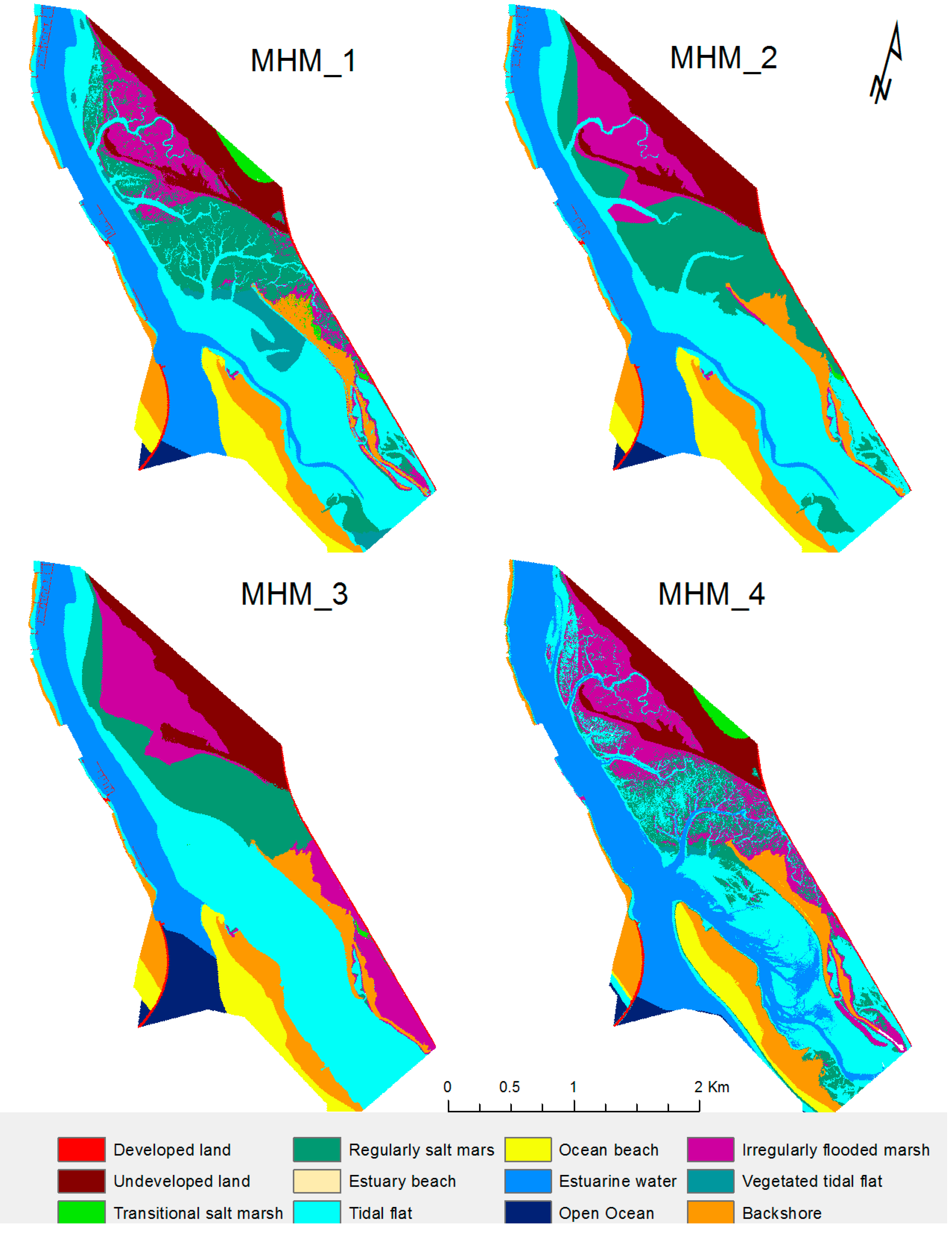
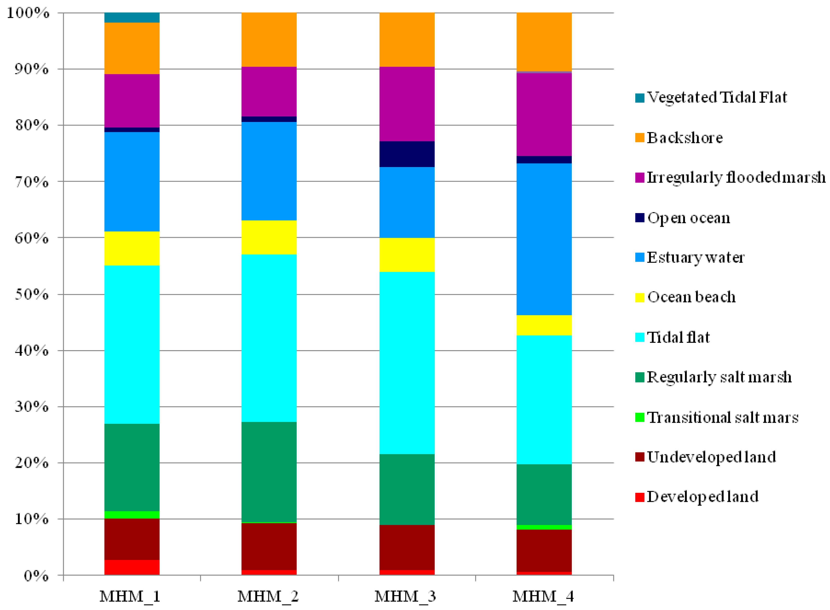
| MHM_1 | Marsh Habitat Map derived from supervised classification using 2013 aerial photography and DEM_2 (1 m spatial resolution) | [31] |
| MHM_2 | Manual simplification of MHM1 (5 m spatial resolution) to remove small creeks (retains main creeks) | Derived from MHM1 (e.g., fewer small creeks) |
| MHM_3 | Manual simplification of MHM2 (5 m spatial resolution) to remove all creeks (only the main tidal channels remain) | Derived from MHM2 (e.g., only the main channel) |
| MHM_4 | Reclassification of DEM2 based on habitat elevation range. For Upland categories and backshore (where the height range overlaps, manual editing was carried out) | Derived from DEM2 |
| EIN | Elevation inputs (EINs) per habitat category (zonation) EIN_a (±0.2 m); EIN_b (±0.4 m) | [32] |
| Input Parameters | |
|---|---|
| Description | Punta Umbría Ria |
| Habitat Map Photo Date (YYYY) | 2013 |
| Digital Elevation Model Date (YYYY) | 2013 |
| Direction Offshore (n, s, e, w) | South |
| Historic Trend (mm/year) | 3.3 |
| Mean Tide Level - Vertical datum (m) | 0.39 |
| Great Diurnal Tide Range (m) | 3.11 |
| Salt Elev. (m above MTL) | 2.09 |
| Marsh Erosion (horz. m/year) | 0.0105 |
| T.Flat Erosion (horz. m/year) | 0.003 |
| Reg. Flood Marsh Accr (mm/year) | 6.57 |
| Irreg. Flood Marsh Accr (mm/year) | 2.5 |
| Description | Test 1 | Test 2 | Test 3 | Test 4 | Test 5 |
|---|---|---|---|---|---|
| Cell size (m) | 3, 5, 10 | 5 | 5 | 5 | 5 |
| Digital Elevation Model | DEM_2 | DEM_2 | DEM_2 | DEM_3 | DEM_1 DEM_2 |
| Marsh Habitat Map | MHM_1 | MHM_1 MHM_2 MHM_3 MHM_4 | MHM_1 | MHM_1 MHM_3 | MHM_1 |
| Elev. Prep * | False | False | False | False/True | False |
| Elevation ranges (zonation) | EIN | EIN | EIN EIN_a (±0.2 m) EIN_b (±0.4 m) | EIN | EIN |
© 2019 by the authors. Licensee MDPI, Basel, Switzerland. This article is an open access article distributed under the terms and conditions of the Creative Commons Attribution (CC BY) license (http://creativecommons.org/licenses/by/4.0/).
Share and Cite
Fernandez-Nunez, M.; Burningham, H.; Díaz-Cuevas, P.; Ojeda-Zújar, J. Evaluating the Response of Mediterranean-Atlantic Saltmarshes to Sea-Level Rise. Resources 2019, 8, 50. https://doi.org/10.3390/resources8010050
Fernandez-Nunez M, Burningham H, Díaz-Cuevas P, Ojeda-Zújar J. Evaluating the Response of Mediterranean-Atlantic Saltmarshes to Sea-Level Rise. Resources. 2019; 8(1):50. https://doi.org/10.3390/resources8010050
Chicago/Turabian StyleFernandez-Nunez, Miriam, Helene Burningham, Pilar Díaz-Cuevas, and José Ojeda-Zújar. 2019. "Evaluating the Response of Mediterranean-Atlantic Saltmarshes to Sea-Level Rise" Resources 8, no. 1: 50. https://doi.org/10.3390/resources8010050
APA StyleFernandez-Nunez, M., Burningham, H., Díaz-Cuevas, P., & Ojeda-Zújar, J. (2019). Evaluating the Response of Mediterranean-Atlantic Saltmarshes to Sea-Level Rise. Resources, 8(1), 50. https://doi.org/10.3390/resources8010050