Abstract
Solar and wind resources available for power generation are subject to variability due to meteorological factors. Here, we use a new global climate reanalysis product, Version 2 of the NASA Modern-Era Retrospective Analysis for Research and Applications (MERRA-2), to quantify interannual variability of monthly-mean solar and wind resource from 1980 to 2016 at a resolution of about 0.5 degrees. We find an average coefficient of variation (CV) of 11% for monthly-mean solar radiation and 8% for wind speed. Mean CVs were about 25% greater over ocean than over land and, for land areas, were greatest at high latitude. The correlation between solar and wind anomalies was near zero in the global mean, but markedly positive or negative in some regions. Both wind and solar variability were correlated with values of climate modes such as the Southern Oscillation Index and Arctic Oscillation, with correlations in the Northern Hemisphere generally stronger during winter. We conclude that reanalysis solar and wind fields could be helpful in assessing variability in power generation due to interannual fluctuations in the solar and wind resource. Skillful prediction of these fluctuations seems to be possible, particularly for certain regions and seasons, given the persistence or predictability of climate modes with which these fluctuations are associated.
1. Introduction
Solar (photovoltaic and thermal) and wind power are rapidly increasing in importance as components of the modern energy grid. Solar and wind resources vary widely in space and time, largely associated with weather factors. There is increasing interest in building on the past century’s advances in numerical weather prediction to forecast solar and wind availability at specific places and times, enabling better matching of energy supply, demand and storage [1,2,3,4].
Forecasting of weather minutes to days ahead is well established. Most applications of solar [5,6,7,8,9,10,11,12,13,14,15,16] and wind [17,18,19] forecasting have been at these shorter durations, developing a wide variety of methods and tools. However, there is also longer-term variability in solar and wind resources, beyond the mean annual cycle. For example, interannual variability in solar resource has been mapped for the United States (U.S.) [20], and monthly and annual wind power resource and production in Portugal respond to large-scale atmospheric circulation patterns, such as the North Atlantic Oscillation [21]. Solar radiation reaching the surface, particularly the direct fraction important for concentrating and thermal solar power applications, varies widely from year to year at some locations, driven by variation in cloudiness and in atmospheric aerosol loading [22]. In the western U.S., atmosphere and ocean circulation patterns led to notably slacker wind than usual in the first half of 2015, a ‘wind drought’, which greatly affected power generation [23].
Weather forecasting at seasonal timescales (roughly one to several months ahead) has also advanced in recent years, exploiting sources of relatively long-range predictability in the climate system [24,25,26,27,28,29]. The main variables forecasted have typically been temperature and precipitation, with monsoon and drought forecasting for agricultural applications being an important focus [30,31,32,33,34,35,36].
The goal of this paper is to better understand global patterns of seasonal-scale interannual variability in wind and solar resources and to consider to what extent this variability might be predictable up to several months in advance. To achieve this, we here (a) map the interannual variability and co-variability of monthly wind and solar resource fields in a global reanalysis product (MERRA-2) and (b) correlate wind and solar variability with values of major climate modes and study their potential predictability.
2. Methods
2.1. Reanalysis Wind and Solar Resource Fields
Version 2 of the NASA Modern-Era Retrospective Analysis for Research and Applications (MERRA-2) estimates the state of the Earth’s atmosphere since 1980 by assimilating extensive meteorological observations to the dynamic climate model GEOS-5, at about 50-km spatial resolution [37,38,39]. Compared to the original MERRA [40], MERRA-2 assimilates a wider range of satellite data and in particular is the first major reanalysis to assimilate satellite aerosol observations [41], which is expected to be particularly useful for accurately representing solar variability in desert and polluted areas. The earlier MERRA product has been used for a study of wind power statistics in Great Britain, which found good correlations between the reanalysis winds and available in situ measurements [42]. Conversion of MERRA and MERRA-2 hourly meteorological variables to wind power and photovoltaic capacity factors, calibrated to available national and site level renewable power generation data, has also been carried out for a set of European countries [43,44].
We analyzed MERRA-2 products at the provided spatial resolution of 0.5° latitude and 0.625° longitude. The mean monthly MERRA-2 field we used as a proxy for solar resource is SWGDN, surface incident shortwave flux. This is expected to be roughly proportional to photovoltaic power production, though for concentrating systems, the direct solar flux is more important. As a proxy for wind resource, we used wind speed at 50-m height (calculated from the hourly easterly and northerly velocity components, U50M and V50M, and averaged to monthly), which is comparable to the typical hub height of commercial wind turbines. In fact, the power available from wind scales as wind speed cubed (whose monthly mean is not provided as a reanalysis field), and real relationships between wind speed and wind power generation are more complicated. Still, it is empirically found that on a monthly timescale, fluctuations in mean wind speed are well correlated with wind power availability and with recorded power generation [23].
As one check on the representation of interannual solar and wind resource variability in MERRA-2, we compared it with available station observations. These observations were obtained from the Global Historical Climatology Network-Daily (GHCN-D) database [45]. Only data not flagged with quality concerns [46] were used. MERRA-2 wind speed (at 10-m height; MERRA-2 variable name: SPEED) was compared with GHCN-D wind speed (AWND). Since few shortwave flux measurements were available in GHCN-D, MERRA-2 shortwave flux was compared with one minus cloud fraction (ACMC, ACMH, ACSC, or ACSH in GHCN-D). The daily GHCN-D values were averaged to monthly, and the comparison was to the MERRA-2 grid cell containing the station coordinates. All stations with complete data for a given month for at least 5 years during the study period (1980 to 2016) were retained, resulting in 1120 usable stations for wind speed and 278 for solar flux. The mean interannual coefficient of variation of the monthly values was 12.2% for wind and 13.8% for solar station measurements. The corresponding values for the subsampled MERRA-2 grid were 8.3% and 6.9%, implying that the interannual variability in MERRA-2 is of the right order of magnitude, though somewhat lower than what is seen at individual stations. The median correlation coefficient between the station and MERRA-2 data interannual variability was 0.458 for wind and 0.469 for solar resource, suggesting that the interannual variability in the MERRA-2 reanalysis is also mostly in phase with that observed on the ground.
We also compared MERRA-2 shortwave flux with the corresponding monthly surface downwelling shortwave radiation product in Version 2 of the Climate Monitoring Satellite Application Facility cLoud, Albedo and RAdiation dataset from Advanced Very High Resolution Radiometer data (CLARA) [47], a EUMETSAT product based on the data record of instruments on polar-orbiting meteorological satellites. CLARA had quasi-global coverage for 1982 to 2015 on a 0.25° grid, which we regridded to the MERRA-2 grid before comparison. The (area-weighted) median correlation coefficient between CLARA and MERRA-2 interannual variability was 0.503, slightly better than the correlation of MERRA-2 with station cloudiness data. The mean interannual coefficients of variation were quite similar (8.0% for subsampled MERRA-2, 8.6% for CLARA).
2.2. Wind and Solar Interannual Variability
For each MERRA-2 pixel, given the mean wind/solar resource for each month and its interannual standard deviation , a coefficient of variation CV was calculated as:
Dividing by the annual mean value, this formula avoids giving too much weight to variability in months when the average resource is low, such as high-latitude winters for solar resource. This CV was mapped, and its mean value was calculated for land and water pixels separately for three approximately equal-area latitude bands: 0° to 19° (low latitude), 19° to 42° (mid latitude), 42° to 90° (high latitude).
Since many power grids now include substantial amounts of both wind and solar generation, we also computed the correlation coefficient (for each grid cell and month of the year separately) between the wind and solar resources. Positive correlation between the two means that months with anomalously low wind resource will likely also have less solar resource than usual, worsening the impact of interannual variability on power supply. Negative correlation means that fluctuations in the two resources will tend to offset each other, potentially mitigating the impact.
2.3. Wind and Solar Associations with Climate Modes and Potential Predictability
A number of recognized modes of variability in the climate system affect climate statistics over large areas throughout the globe. Here, we perform a preliminary assessment of the extent to which solar and wind anomalies are associated with each of these climate modes. We do this by computing the adjusted coefficient of determination between MERRA-2 solar or wind resource and the value of each climate mode, where is calculated using the Pratt formula and intended to be an approximately unbiased measure [48,49,50] of what fraction of the resource variance could be explained by variability in the climate mode. Adjusted correlation is obtained as with the sign being the same as the unadjusted correlation, or 0 if . was computed separately for each MERRA-2 grid cell and for each month of the year and then averaged to assess variation between land and ocean and by latitude and season. This was also computed for previous climate mode values (lagged up to 12 months) to provide an indication of the extent to which future solar and wind resource fluctuations could be predicted given present conditions.
Note that for each grid cell and month, and assuming that resource and climate mode values from the 37 years are independent and normally distributed, ( corresponding to unadjusted ) is significantly different from zero at the 0.95 confidence level.
The five climate modes chosen were those for which monthly index values, calculated from atmospheric pressure and sea surface temperature (SST) fields, were available from the U.S. National Oceanic and Atmospheric Administration (NOAA) [51]. In alphabetical order, they are:
- Arctic Oscillation (AO), a mode of surface-pressure variability between the Arctic and North Atlantic and Pacific [52].
- North Atlantic Oscillation (NAO), a mode of 500-millibar (mb) height variability between Greenland and the central North Atlantic [53].
- Pacific Decadal Oscillation (PDO), a mode of North Pacific SST variability [54].
- Pacific-North America Index (PNA), a mode of 500-mb height variability between the North Pacific and western North America [55].
- Southern Oscillation Index (SOI), surface pressure variability across the tropical Pacific [56].
2.4. Interannual Variability over Longer Aggregation Periods
Most of the analysis in this paper is for the variability of monthly-mean solar radiation and wind speed. To begin to extend this to longer-lasting variability, such as the 2015 western USA wind drought (which lasted about 6 months) [23], we computed the CV also for 2- to 12-month aggregation periods. The mean CV is expected to decrease with increasing aggregation period, with the rate of decrease depending both on the autocorrelation of anomalies in consecutive months (which we found to be small, but positive) and on any long-term ‘memory’ due to, for example, the association of anomalies with long-lasting climate modes.
3. Results
3.1. Interannual Variability
The global mean (area-weighted) coefficient of variation, defined as above, was 8% for monthly solar radiation and 11% for wind speed. Across latitude bands, variability was greater, on average, over water than over land (Table 1). Solar variability was lowest in mid latitudes compared to high and low latitudes. Wind variability peaked in low latitudes over water, but at high latitudes over land (Table 1).

Table 1.
Mean coefficient of variation (%) for monthly wind and solar resource, by latitude band.
Within these broad latitudinal and land/water patterns, solar radiation showed low variability over deserts and subtropical oceans with generally sunny conditions and relatively high variability over much of tropical and temperate Eurasia (Figure 1a). Wind speed interannual variability was high over and offshore of Europe as well as in the Equatorial oceans, and greater over mountainous western North America compared to the flatter east (Figure 1b). More broadly, wind variability, but not solar variability, appeared to be greater over mountainous regions globally.
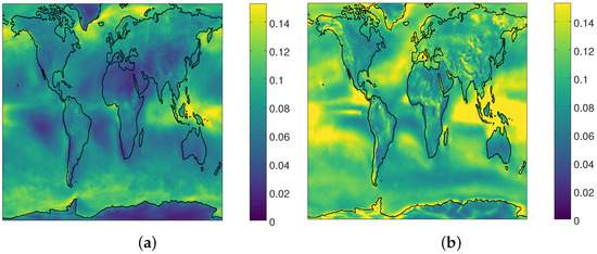
Figure 1.
Interannual coefficient of variation for monthly surface (a) solar radiation and (b) wind speed.
A sense of seasonal differences in the coefficients of variation is conveyed by Figure 2, which shows the ratio of January to July CVs. In general, rainy seasons (winter in Mediterranean climates and summer in tropical and monsoon regions) show higher CVs than dry seasons. Europe tends to have more variability in winter as compared to summer, while South and East Asia tend to be the opposite, and North America is mixed.
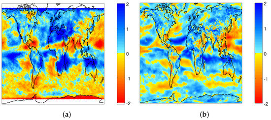
Figure 2.
Base-2 logarithm of the ratio between January and July interannual coefficient of variation for surface (a) solar radiation and (b) wind speed. A value of for example, means that the CV is twice as large in January, while with a value of the CV is twice as large in July.
Wind and solar anomalies tended to be negatively correlated with each other over the mid- and high-latitude oceans, but positively correlated over low-latitude land (Table 2). Mean correlations were strongly positive (around 0.4) over much of tropical South America, Africa, Indonesia and India, as well as over Mexico and the adjoining southwest U.S. and east China (Figure 3). In those areas, which include many of the regions that are most intensely developing wind and solar resources, the interannual variability of wind and solar resources is expected to often be in phase, increasing the impact of climate fluctuations on energy supply. On the other hand, these correlations were negative in Europe and Siberia, implying that solar resource development there could reduce fluctuations in energy supply due to interannual variations in wind speed.
Table 2.
Mean correlation coefficient between wind and solar resource monthly anomalies, by latitude band.
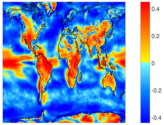
Figure 3.
Mean correlation between anomalies in monthly surface solar radiation and wind speed.
3.2. Association with Climate Modes and Predictability
Averaged over all land areas, the estimated fraction of variance in the monthly anomaly fields that could be explained by linear regression with the climate modes, was greatest for SOI in the case of solar radiation and greatest for AO for wind speed (Table 3). SOI was the climate mode best associated with wind and solar variability at low latitudes, but explained little of the variance at high latitudes, where AO and NAO were the best associated. PDO was similar to SOI in having the strongest associations at low latitudes, while PNA had latitudinally more uniform and generally weaker correlations (Table 3).
Table 3.
Mean % variability ( of linear regression) in monthly surface solar radiation and wind speed that could be explained by large-scale climate modes, by latitude band. AO, Arctic Oscillation; NAO, North Atlantic Oscillation; PDO, Pacific Decadal Oscillation; PNA, Pacific-North America Index; SOI, Southern Oscillation Index.
Many of these associations showed a marked seasonal variation in strength. In particular, over high-latitude land areas, AO and NAO were strongly correlated with solar and wind variability in December to March, with AO showing particularly good correlations with wind variability, whereas mean correlations in other months were much weaker (Figure 4).
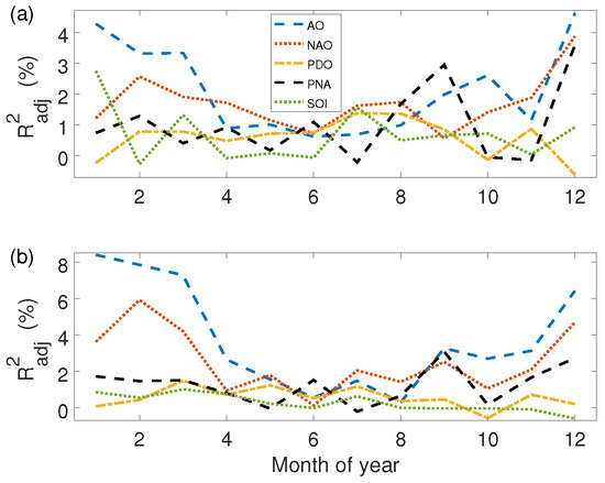
Figure 4.
Mean high-latitude land for correlation between monthly (a) solar radiation or (b) wind speed and values for climate modes of the same month, by time of year.
Even within latitude zones, associations are spatially quite non-uniform. For example, AO shows high associations () in winter with solar radiation and wind speed in the North Atlantic, Northern Europe, the western Mediterranean and the Sahara, but much smaller associations in North America (Figure 5). NAO is correlated with winter wind speed particularly around the North and Baltic seas (Figure 6) and PDO over the western Mediterranean and northern China (Figure 7). On the other hand, the PNA is strongly associated with winter wind anomalies over much of the U.S., but not over Europe (Figure 8). SOI is strongly correlated with solar and wind anomalies in the tropical Pacific, but also with winter anomalies in the south-central U.S. (Figure 9).
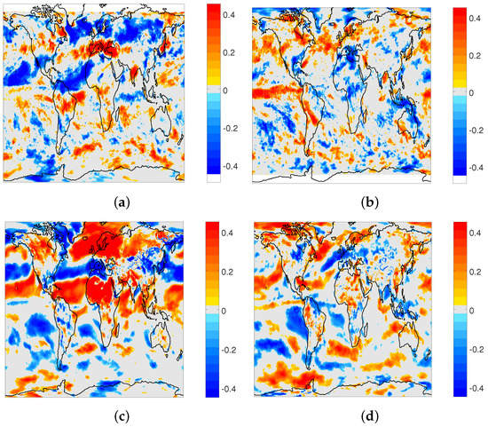
Figure 5.
for correlation with AO with (a) solar radiation in January; (b) solar radiation in July; (c) wind speed in January; (d) wind speed in July.
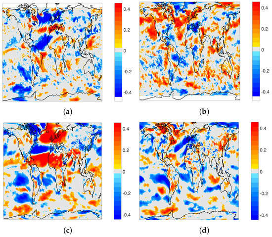
Figure 6.
Same as Figure 5, but for correlation with NAO.
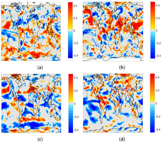
Figure 7.
Same as Figure 5, but for correlation with PDO.
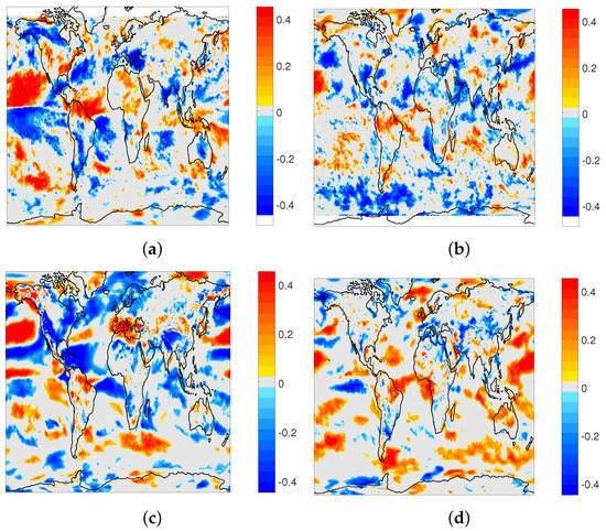
Figure 8.
Same as Figure 5, but for correlation with PNA.
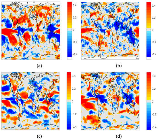
Figure 9.
Same as Figure 5, but for correlation with SOI.
The results presented so far are for associations between climate modes and solar and wind anomalies from the same month. Solar and wind anomalies can also be associated, to varying extents, with climate mode values from previous months (Figure 10). AO and NAO are not very persistent across multiple months, and so, the correlation strengths diminish rapidly as one goes earlier than the current month. SOI and especially PDO are persistent across months, so correlations decay more slowly, implying that future wind and solar anomalies should be partly predictable based on current values of these climate modes (Figure 10).
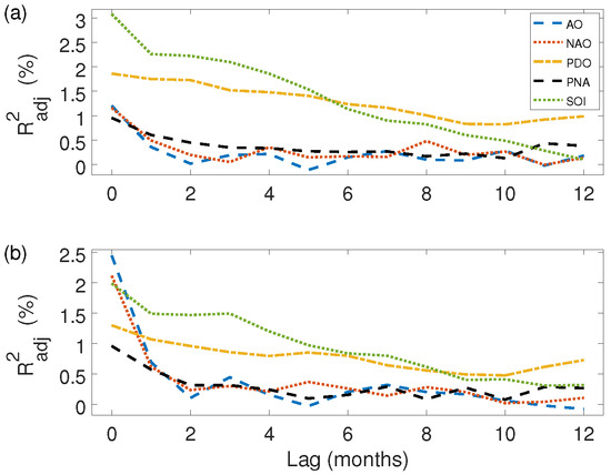
Figure 10.
Global mean land for correlation between monthly (a) solar radiation or (b) wind speed and values for different climate modes up to 12 months prior.
3.3. Longer Aggregation Periods
The magnitude of interannual variation in mean solar radiation and wind speed decreases as we increase the aggregation period length, as expected. The decrease is less rapid than would be expected if mean solar radiation and wind speed anomalies followed an autoregressive process of order one where autocorrelations fell off exponentially (Figure 11). This tendency can be attributed at least in part to the association of these anomalies with long-lasting climate modes such as SOI and PDO, and it makes long-lasting fluctuations such as multi-month regional wind drought more likely than might be calculated if anomalies were modeled as an AR(1) process.
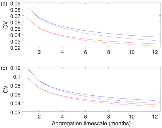
Figure 11.
Global mean land (red) and ocean (blue) coefficient of variation between monthly (a) solar radiation or (b) wind speed at aggregation timescales of one to 12 months. The expected values for an autoregressive process of order one that matches the one- and two-month values are also shown (dashed curves).
4. Discussion
The global-mean coefficients of variation for monthly-mean solar radiation and wind speed in the MERRA-2 reanalysis were found to be 11% and 8%, respectively. While variability was lower on average over land than over oceans, some of the land areas that currently have the largest build-up of solar and wind energy generation, e.g., in India, China, Western Europe and the U.S., had greater than average variability. Variability is expected to be greater at the scale of individual generation plants, compared to the reanalysis grid scale, as also hinted at by the larger median coefficients of variation in station observations compared to MERRA-2.
A full assessment of the impact of monthly-scale resource variability on wind and solar energy generation at a particular site or power grid would benefit from in situ observation series, as well as consideration of the power curves of specific generation equipment that takes into account, e.g., the proportionality of available power to the cube of wind speed and the reliance of solar thermal equipment on the direct fraction of solar radiation. Nevertheless, based on our comparison with GHCN-D station and CLARA remote sensing observations and the finding that the 2015 wind drought experienced by wind power operators in the western U.S. can be seen in MERRA-2 near-surface wind speed [23], the reanalysis products presented here appear to be useful in providing approximate numerical values for initial assessment of the magnitude of interannual variability and its impact on reliability and storage requirements [57].
Both wind and solar monthly anomalies were found to show some correlation with the climate modes tested. To the extent that these climate modes are persistent or dynamically predictable, long-range forecasts of these anomalies are possible. Statistical and dynamical methods can be used to predict sea surface temperatures [30,58,59], which are strongly associated with many of the climate modes, and there are also other sources of seasonal predictability, for example related to snow cover and soil moisture [60,61]. Thus, improvements in NAO forecasting have led to better winter wind power forecasts over Europe [62].
Many of the teleconnection correlations, particularly those for AO and NAO in winter (Figure 5 and Figure 6), are of opposite sign between Northern and Southern Europe, implying that spreading and interconnecting wind and solar generation across the continent can mitigate the impact of interannual variability on power supply. Similarly, positive correlations between wind and solar variability, such as that seen in the southwestern U.S., can suggest the need for additional provision for reserve power or grid interconnections.
Predictability based on these climate modes is seen to be much greater for some locations and seasons than is the case in the global mean. The climate modes used here, taken from NOAA, are ones that are known to influence weather in the U.S. For other locations, for example in the Southern Hemisphere, other climate modes, such as the Antarctic Oscillation [63], could have stronger associations with wind and solar fluctuations.
5. Conclusions
We find a substantial amount of interannual variability, with mean coefficients of variation of order 10% at the monthly timescale, in both solar radiation and wind speed, which could result in important fluctuations in the supplied power from solar and wind resources. Some of this variability correlates with the values of climate modes, and the persistence and predictability of these modes provides the potential for skill in seasonal prediction of these wind and solar fluctuations.
Acknowledgments
Nir Y. Krakauer gratefully acknowledges support from NOAA under Grants NA11SEC4810004 and NA15OAR4310080. The authors thank Daran Rife for valuable comments and help with datasets and the participants in the American Solar Energy Society annual conference for helpful discussion. All statements made are the views of the authors and not the opinions of the funders nor the U.S. government.
Author Contributions
Nir Y. Krakauer and Daniel S. Cohan conceived of and designed the data analysis and contributed analysis tools. Nir Y. Krakauer performed the data analysis and wrote the paper.
Conflicts of Interest
The authors declare no conflict of interest.
References
- Kostylev, V.; Pavlovski, A. Solar power forecasting performance—Towards industry standards. In Proceedings of the 1st International Workshop on the Integration of Solar Power into Power Systems, Aarhus, Denmark, 24 October 2011. [Google Scholar]
- Masa-Bote, D.; Castillo-Cagigal, M.; Matallanas, E.; Caamaño-Martín, E.; Gutiérrez, A.; Monasterio-Huelín, F.; Jiménez-Leube, J. Improving photovoltaics grid integration through short time forecasting and self-consumption. Appl. Energy 2014, 125, 103–113. [Google Scholar] [CrossRef]
- Widén, J.; Carpman, N.; Castellucci, V.; Lingfors, D.; Olauson, J.; Remouit, F.; Bergkvist, M.; Grabbe, M.; Waters, R. Variability assessment and forecasting of renewables: A review for solar, wind, wave and tidal resources. Renew. Sustain. Energy Rev. 2015, 44, 356–375. [Google Scholar] [CrossRef]
- Juban, R.; Ohlsson, H.; Maasoumy, M.; Poirier, L.; Kolter, J.Z. A multiple quantile regression approach to the wind, solar, and price tracks of GEFCom2014. Int. J. Forecast. 2016, 32, 1094–1102. [Google Scholar] [CrossRef]
- Hammer, A.; Heinemann, D.; Lorenz, E.; Lückehe, B. Short-term forecasting of solar radiation: A statistical approach using satellite data. Sol. Energy 1999, 67, 139–150. [Google Scholar] [CrossRef]
- Sfetsos, A.; Coonick, A.H. Univariate and multivariate forecasting of hourly solar radiation with artificial intelligence techniques. Sol. Energy 2000, 68, 169–178. [Google Scholar] [CrossRef]
- Perez, R.; Moore, K.; Wilcox, S.; Renné, D.; Zelenka, A. Forecasting solar radiation–Preliminary evaluation of an approach based upon the national forecast database. Sol. Energy 2007, 81, 809–812. [Google Scholar] [CrossRef]
- Reikard, G. Predicting solar radiation at high resolutions: A comparison of time series forecasts. Sol. Energy 2009, 83, 342–349. [Google Scholar] [CrossRef]
- Mellit, A.; Pavan, A.M. A 24-h forecast of solar irradiance using artificial neural network: Application for performance prediction of a grid-connected PV plant at Trieste, Italy. Sol. Energy 2010, 84, 807–821. [Google Scholar] [CrossRef]
- Mathiesen, P.; Kleissl, J. Evaluation of numerical weather prediction for intra-day solar forecasting in the continental United States. Sol. Energy 2011, 86, 967–977. [Google Scholar] [CrossRef]
- Chow, C.W.; Urquhart, B.; Lave, M.; Dominguez, A.; Kleissl, J.; Shields, J.; Washom, B. Intra-hour forecasting with a total sky imager at the UC San Diego solar energy testbed. Sol. Energy 2011, 85, 2881–2893. [Google Scholar] [CrossRef]
- Yang, D.; Gu, C.; Dong, Z.; Jirutitijaroen, P.; Chen, N.; Walsh, W.M. Solar irradiance forecasting using spatial-temporal covariance structures and time-forward kriging. Renew. Energy 2013, 60, 235–245. [Google Scholar] [CrossRef]
- Isvoranu, D.; Badescu, V. Preliminary WRF-ARW model analysis of global solar irradiation forecasting. Math. Model. Civ. Eng. 2014, 10, 1–8. [Google Scholar] [CrossRef]
- Chu, Y.; Li, M.; Pedro, H.T.; Coimbra, C.F. Real-time prediction intervals for intra-hour DNI forecasts. Renew. Energy 2015, 83, 234–244. [Google Scholar] [CrossRef]
- Larson, D.P.; Nonnenmacher, L.; Coimbra, C.F. Day-ahead forecasting of solar power output from photovoltaic plants in the American Southwest. Renew. Energy 2016, 91, 11–20. [Google Scholar] [CrossRef]
- Golestaneh, F.; Gooi, H.B.; Pinson, P. Generation and evaluation of space–time trajectories of photovoltaic power. Appl. Energy 2016, 176, 80–91. [Google Scholar] [CrossRef]
- Lange, M. On the uncertainty of wind power predictions–analysis of the forecast accuracy and statistical distribution of errors. J. Sol. Energy Eng. 2005, 127, 177–184. [Google Scholar] [CrossRef]
- Hering, A.S.; Genton, M.G. Powering up with space-time wind forecasting. J. Am. Stat. Assoc. 2010, 105, 92–104. [Google Scholar] [CrossRef]
- Gallego-Castillo, C.; Bessa, R.; Cavalcante, L.; Lopez-Garcia, O. On-line quantile regression in the RKHS (Reproducing Kernel Hilbert Space) for operational probabilistic forecasting of wind power. Energy 2016, 113, 355–365. [Google Scholar] [CrossRef]
- Gueymard, C.A.; Wilcox, S.M. Assessment of spatial and temporal variability in the US solar resource from radiometric measurements and predictions from models using ground-based or satellite data. Sol. Energy 2011, 85, 1068–1084. [Google Scholar] [CrossRef]
- Correia, J.; Bastos, A.; Brito, M.; Trigo, R. The influence of the main large-scale circulation patterns on wind power production in Portugal. Renew. Energy 2017, 102 Pt A, 214–223. [Google Scholar] [CrossRef]
- Gueymard, C.A. Temporal variability in direct and global irradiance at various time scales as affected by aerosols. Sol. Energy 2012, 86, 3544–3553. [Google Scholar] [CrossRef]
- Rife, D.; Krakauer, N.Y.; Cohan, D.S.; Collier, J.C. A new kind of drought: U.S. record low windiness in 2015. Earthzine 2016. Available online: https://earthzine.org/2016/06/10/a-new-kind-of-drought-u-s-record-low-windiness-in-2015/ (accessed on 18 July 2017).
- Koster, R.D.; Suarez, M.J.; Heiser, M. Variance and predictability of precipitation at seasonal-to-interannual timescales. J. Hydrometeorol. 2000, 1, 26–46. [Google Scholar] [CrossRef]
- National Research Council. Assessment of Intraseasonal to Interannual Climate Prediction and Predictability; Technical Report; National Academies Press: Washington, DC, USA, 2010. [Google Scholar]
- Troccoli, A. Seasonal climate forecasting. Meteorol. Appl. 2010, 17, 251–268. [Google Scholar] [CrossRef]
- Smith, D.M.; Scaife, A.A.; Kirtman, B.P. What is the current state of scientific knowledge with regard to seasonal and decadal forecasting? Environ. Res. Lett. 2012, 7, 015602. [Google Scholar] [CrossRef]
- Doblas-Reyes, F.J.; García-Serrano, J.; Lienert, F.; Biescas, A.P.; Rodrigues, L.R.L. Seasonal climate predictability and forecasting: Status and prospects. Wiley Interdiscip. Rev. Clim. Chang. 2013, 4. [Google Scholar] [CrossRef]
- Committee on Developing a U.S. Research Agenda to Advance Subseasonal to Seasonal Forecasting; Board on Atmospheric Sciences and Climate; Ocean Studies Board; Division on Earth and Life Studies; National Academies of Sciences, Engineering, and Medicine. Next Generation Earth System Prediction: Strategies for Subseasonal to Seasonal Forecasts; National Academies Press: Washington, DC, USA, 2016. [Google Scholar]
- Barnston, A.G.; Mason, S.J.; Goddard, L.; Dewitt, D.G.; Zebiak, S.E. Multimodel ensembling in seasonal climate forecasting at IRI. Bull. Am. Meteorol. Soc. 2003, 84, 1783–1796. [Google Scholar] [CrossRef]
- Kumar, K.K.; Hoerling, M.; Rajagopalan, B. Advancing dynamical prediction of Indian monsoon rainfall. Geophys. Res. Lett. 2005, 32, L08704. [Google Scholar]
- Barnston, A.G.; Li, S.; Mason, S.J.; DeWitt, D.G.; Goddard, L.; Gong, X. Verification of the first 11 years of IRI’s seasonal climate forecasts. Appl. Meteorol. Climatol. 2010, 49, 493–520. [Google Scholar] [CrossRef]
- Barnston, A.G.; Mason, S.J. Evaluation of IRI’s seasonal climate forecasts for the extreme 15% tails. Weather Forecast. 2011, 26, 545–554. [Google Scholar] [CrossRef]
- Mwangi, E.; Wetterhall, F.; Dutra, E.; Di Giuseppe, F.; Pappenberger, F. Forecasting droughts in East Africa. Hydrol. Earth Syst. Sci. 2014, 18, 611–620. [Google Scholar] [CrossRef]
- Dutra, E.; Pozzi, W.; Wetterhall, F.; Di Giuseppe, F.; Magnusson, L.; Naumann, G.; Barbosa, P.; Vogt, J.; Pappenberger, F. Global meteorological drought—Part 2: Seasonal forecasts. Hydrol. Earth Syst. Sci. 2014, 18, 2669–2678. [Google Scholar] [CrossRef]
- Klemm, T.; McPherson, R.A. The development of seasonal climate forecasting for agricultural producers. Agric. Forest Meteorol. 2017, 232, 384–399. [Google Scholar] [CrossRef]
- Bosilovich, M.G.; Robertson, F.R.; Takacs, L.; Molod, A.; Mocko, D. Atmospheric Water Balance and Variability in the MERRA-2 Reanalysis. J. Clim. 2017. [Google Scholar] [CrossRef]
- Reichle, R.H.; Liu, Q.; Koster, R.D.; Draper, C.S.; Mahanama, S.P.P.; Partyka, G.S. Land surface precipitation in MERRA-2. J. Clim. 2017. [Google Scholar] [CrossRef]
- Wargan, K.; Coy, L. Strengthening of the Tropopause Inversion Layer during the 2009 Sudden Stratospheric Warming: A MERRA-2 Study. J. Atmos. Sci. 2016, 73, 1871–1887. [Google Scholar] [CrossRef]
- Rienecker, M.M.; Suarez, M.J.; Gelaro, R.; Todling, R.; Bacmeister, J.; Liu, E.; Bosilovich, M.G.; Schubert, S.D.; Takacs, L.; Kim, G.K.; et al. MERRA: NASA’s modern-era retrospective analysis for research and applications. J. Clim. 2011, 24. [Google Scholar] [CrossRef]
- Randles, C.A.; da Silva, A.M.; Buchard, V.; Colarco, P.R.; Darmenov, A.; Govindaraju, R.; Smirnov, A.; Holben, B.; Ferrare, R.; Hair, J.; et al. The MERRA-2 Aerosol Reanalysis, 1980—Onward, Part I: System Description and Data Assimilation Evaluation. J. Clim. 2017. [Google Scholar] [CrossRef]
- Cannon, D.; Brayshaw, D.; Methven, J.; Coker, P.; Lenaghan, D. Using reanalysis data to quantify extreme wind power generation statistics: A 33 year case study in Great Britain. Renew. Energy 2015, 75, 767–778. [Google Scholar] [CrossRef]
- Staffell, I.; Pfenninger, S. Using bias-corrected reanalysis to simulate current and future wind power output. Energy 2016, 114, 1224–1239. [Google Scholar] [CrossRef]
- Pfenninger, S.; Staffell, I. Long-term patterns of European PV output using 30 years of validated hourly reanalysis and satellite data. Energy 2016, 114, 1251–1265. [Google Scholar] [CrossRef]
- Menne, M.; Durre, I.; Vose, R.; Gleason, B.; Houston, T. An overview of the Global Historical Climatology Network-Daily database. J. Atmos. Ocean. Technol. 2012, 29, 897–910. [Google Scholar] [CrossRef]
- Durre, I.; Menne, M.J.; Gleason, B.E.; Houston, T.G.; Vose, R.S. Comprehensive automated quality assurance of daily surface observations. J. Appl. Meteorol. Climatol. 2010, 49, 1615–1633. [Google Scholar] [CrossRef]
- Karlsson, K.G.; Riihelä, A.; Müller, R.; Meirink, J.F.; Sedlar, J.; Stengel, M.; Lockhoff, M.; Trentmann, J.; Kaspar, F.; Hollmann, R.; et al. CLARA-A1: A cloud, albedo, and radiation dataset from 28 year of global AVHRR data. Atmos. Chem. Phys. 2013, 13, 5351–5367. [Google Scholar] [CrossRef]
- Olkin, I.; Pratt, J.W. Unbiased Estimation of Certain Correlation Coefficients. Ann. Math. Statist. 1958, 29, 201–211. [Google Scholar] [CrossRef]
- Yin, P.; Fan, X. Estimating R2 Shrinkage in Multiple Regression: A Comparison of Different Analytical Methods. J. Exp. Educ. 2001, 69, 203–224. [Google Scholar] [CrossRef]
- Skidmore, S.T.; Thompson, B. Choosing the best correction formula for the Pearson r2 effect size. J. Exp. Educ. 2011, 79, 257–278. [Google Scholar] [CrossRef]
- NOAA-NCEI. Teleconnections. Available online: https://www.ncdc.noaa.gov/teleconnections/ (accessed on 18 July 2017).
- Baldwin, M.P. Annular modes in global daily surface pressure. Geophys. Res. Lett. 2001, 28, 4115–4118. [Google Scholar] [CrossRef]
- Hurrell, J.W.; Kushnir, Y.; Visbeck, M. The North Atlantic Oscillation. Science 2001, 291, 603–605. [Google Scholar] [CrossRef] [PubMed]
- Mantua, N.J.; Hare, S.R. The Pacific Decadal Oscillation. J. Oceanogr. 2002, 58, 35–44. [Google Scholar] [CrossRef]
- Wallace, J.M.; Gutzler, D.S. Teleconnections in the Geopotential Height Field during the Northern Hemisphere Winter. Mon. Weather Rev. 1981, 109, 784–812. [Google Scholar] [CrossRef]
- Horel, J.D.; Wallace, J.M. Planetary-Scale Atmospheric Phenomena Associated with the Southern Oscillation. Mon. Weather Rev. 1981, 109, 813–829. [Google Scholar] [CrossRef]
- Perez, M.J.R.; Fthenakis, V. Impacts of long-timescale variability in solar resources at high PV penetrations: Quantification. In Proceedings of the 2012 38th IEEE Photovoltaic Specialists Conference (PVSC), Austin, TX, USA, 3–8 June 2012; pp. 002481–002486. [Google Scholar]
- Krishnamurti, T.N.; Chakraborty, A.; Krishnamurti, R.; Dewar, W.K.; Clayson, C.A. Seasonal prediction of sea surface temperature anomalies using a suite of 13 coupled atmosphere-ocean models. J. Clim. 2006, 19, 6069–6088. [Google Scholar] [CrossRef]
- Kumar, A.; Chen, M.; Zhang, L.; Wang, W.; Xue, Y.; Wen, C.; Marx, L.; Huang, B. An analysis of the nonstationarity in the bias of sea surface temperature forecasts for the NCEP Climate Forecast System (CFS) Version 2. Mon. Weather Rev. 2012, 140, 3003–3016. [Google Scholar] [CrossRef]
- Douville, H. Relevance of soil moisture for seasonal atmospheric predictions: Is it an initial value problem? Clim. Dyn. 2004, 22, 429–446. [Google Scholar] [CrossRef]
- Wang, S.; Yuan, X.; Li, Y. Does a strong El Niño imply a higher predictability of extreme drought? Sci. Rep. 2017, 7, 40741. [Google Scholar] [CrossRef] [PubMed]
- Clark, R.T.; Bett, P.E.; Thornton, H.E.; Scaife, A.A. Skilful seasonal predictions for the European energy industry. Environ. Res. Lett. 2017, 12, 024002. [Google Scholar] [CrossRef]
- Gong, D.; Wang, S. Definition of Antarctic Oscillation index. Geophys. Res. Lett. 1999, 26, 459–462. [Google Scholar] [CrossRef]


© 2017 by the authors. Licensee MDPI, Basel, Switzerland. This article is an open access article distributed under the terms and conditions of the Creative Commons Attribution (CC BY) license (http://creativecommons.org/licenses/by/4.0/).