Resource-Oriented Prioritisation of Water-Supply Pipe Groups Using Repair and Service-Interruption Burdens

Abstract

Long utility records support renewal screening when failures, durations and exposure use consistent definitions. An audit covered 4885 water-supply failures in a major city in south-eastern Poland (2004–2025); 4859 had a valid repair duration and 4832 had a valid service-interruption status/duration. Events and annual exposure used the same diameter-based functional classification. Material was identified for 4824 events; 4806 events formed 14 material–function groups. The core CRITIC–TOPSIS model combined exposure-normalised failure rate, mean repair time and mean interruption time; 2000 event-level bootstrap replicates quantified sampling uncertainty. Network length increased by about 84.4%, while failure rate decreased (Spearman ρ = −0.911, p < 0.001). Mean repair and interruption times were 7.96 and 2.43 h; 64.2% of repairs equalled 8 h. Galvanised-steel service connections ranked first (CC = 0.819; P(rank 1) = 0.800; P(top 3) = 1.000), followed by steel and asbestos cement distribution pipes. Product-containing structures and the strict >8, >10 and >12 h threshold variants selected asbestos cement distribution pipes, whereas the inclusive ≥8 h and positive-only SIT variants retained galvanised-steel service connections. The result is a group-screening signal, not a renewal prescription; hydraulic consequence, customers affected, condition and cost remain necessary for segment decisions. Beyond the case study, the workflow provides a transferable, low-data screening approach for directing limited maintenance and renewal resources while accounting for water-service accessibility; numerical priorities should be recalculated using local exposure, operational conditions and decision thresholds.

1. Introduction

Drinking-water distribution systems are expected to provide continuous service while their buried components age under incomplete information. A pipe failure is therefore both a physical event and an operational episode: crews must locate and repair the defect, and users may experience an interruption with a duration that does not necessarily equal the repair duration. Service-quality and utility-management standards consequently treat continuity as an explicit performance dimension rather than an incidental by-product of maintenance [1,2].

Research on water-pipe deterioration has developed from statistical break models to machine learning, survival and probabilistic frameworks. Reviews identify material, diameter, age, pressure, soil, climate, installation and prior failures as relevant predictors [3,4,5]. The predictor sets and data requirements summarised in recent reviews [6,7], together with probabilistic analysis [8], show that model results depend on the content and consistency of the available records. These advances are valuable for failure prediction, but they do not by themselves translate a routine repair log into a transparent operational priority list.

Rehabilitation research generally combines likelihood and consequence. Risk-based and hydraulic criticality methods can identify pipes whose failure would reduce pressure or supply [9,10]. Graph-theoretic and minimum-pressure rankings add topology and resilience information [11,12]. Their practical strength is also a limitation for utilities without a calibrated hydraulic model, complete customer-demand allocation or reliable segment-condition data. A complementary first-stage screen can instead use routinely recorded occurrence, repair and shut-off information, provided that exposure denominators, missingness and uncertainty are handled explicitly.

From a resource-management perspective, water-pipe failures affect more than the physical condition of buried infrastructure. Recurrent failures mobilise maintenance labour, equipment, repair materials and financial resources, while service interruptions temporarily restrict users’ access to treated drinking water. Maintenance and renewal planning therefore involves the allocation of limited operational and capital resources among competing parts of the network. A screening framework that combines exposure-normalised failure occurrence with repair and service-interruption duration can support resource stewardship by identifying pipe groups in which recurring failures generate the greatest operational and service burdens.

The primary CRITIC–TOPSIS model therefore used three non-redundant criteria: exposure-normalised failure rate, mean repair duration and mean service-interruption duration. A six-criterion formulation that additionally included a repair-time threshold and two deterministic products, the Repair Burden Index (RBI = failure rate × mean repair duration) and Service-Interruption Burden Index (SIBI = failure rate × mean interruption duration), was evaluated only as a structural sensitivity variant. Event-level bootstrap resampling provided probabilities and intervals for ranks and scores.

The aim is to develop and test a reproducible operational screening framework for pipe function–material groups using a 22-year failure register.

The specific objectives are to:

• Audit all source records and report outcome-specific denominators;
• Assess temporal comparability, network exposure and repair-time heaping;
• Compare statistically defined pipe, material, diameter and cause groups;
• Evaluate criterion dependence and ranking sensitivity;
• Quantify priority uncertainty and temporal stability.

The methodological contribution is the integration of these audit, uncertainty and sensitivity steps around established CRITIC and TOPSIS procedures.

2. Literature Review

2.1. Pipe Failure, Criticality and Rehabilitation

Failure modelling and rehabilitation prioritisation answer related but different questions. Failure models estimate the probability or timing of an event from pipe and operational predictors [3,4,5], with recent work extending the evidence on data quality and probabilistic factors [6,7,8]. Rehabilitation models additionally require consequence, feasibility and budget information. Raspati et al. combined break probability with inability to supply water [9], whereas Prasad used supply shortage, pressure decline, energy loss and hydraulic uniformity to identify critical pipes [10]. Pagano et al. aggregated graph-theory indicators through a Bayesian belief network [11], and minimum-pressure analysis has recently been used to rank individual critical pipes [12]. These methods show why a high failure rate alone is not an adequate proxy for consequence.

Operational group screening has a different resolution. It identifies material–function classes that repeatedly consume repair resources or generate interruptions, after which the utility can inspect the individual segments within those classes. Group results cannot reproduce hydraulic connectivity, isolation-valve configuration or the number and vulnerability of users affected. Their role is therefore to reduce a large asset portfolio to a documented investigation list, consistent with risk-based rehabilitation practice but not equivalent to segment-level risk.

2.2. Repair Duration and Service Interruption

Repair duration is sensitive to its operational definition. Notification-to-restoration time, crew work time and excavation-to-completion time are not interchangeable. Recent studies have used machine learning to predict supply-interruption duration [13], while resilience-based assessment has been used to evaluate water-supply safety [14], and monitoring research has shown that the waiting component can materially affect MTTR [15]. This study uses the recorded repair work window.

Service-interruption duration is analysed separately. An eight-hour repair can occur without a shut-off, and a shorter technical intervention can interrupt many users if isolation is hydraulically consequential. Hazard-assessment research similarly treats interruption of water supply as one element of wider waterworks-system risk and operational security [16].

An earlier article analysed repair and restoration times for the same local system in 2004–2007 [17]. The present study extends observation through 2025, re-audits the event-level intervals, aligns occurrence with annual material–function exposure, separates repair from service interruption and adds adjusted, uncertainty and sensitivity analyses.

Earlier repair-time research identifies diameter, material, damage type, pavement, repair-team capacity and concurrent failures as potential determinants of the time required to restore a water-supply pipe [18]. These factors support the covariate and limitation framework used here, but most are not consistently available in the historical register.

2.3. Multi-Criteria Prioritisation and Uncertainty

Across roughly two decades, MCDA sorting, method comparison, and analytical-network procedures have been applied to pipe rehabilitation [19,20,21]. Engineering guidance and integrated asset-management frameworks place these rankings within staged investigation and investment decisions [22,23], while a recent qualitative risk model addresses unreliable operational data [24]. These perspectives differ in scale and data availability, but all distinguish portfolio screening from a final intervention decision.

AHP and its network extension elicit relative importance through pairwise judgements, whereas TOPSIS ranks alternatives by distance from ideal and anti-ideal profiles. Fuzzy TOPSIS represents linguistic or imprecise judgements with membership functions and has been applied to water-supply alternatives [25,26]. The present data are observed numerical event records. Sampling uncertainty is addressed directly by event-level bootstrap resampling. CRITIC derives objective weights from criterion contrast and conflict [27], and conventional TOPSIS supplies the relative closeness score [28,29]. These procedures do not remove the analyst’s responsibility to define non-redundant criteria and meaningful alternatives.

TOPSIS ranks can change with uncertain inputs, thresholds, weights or the alternative set. Robustness, uncertainty and sensitivity should therefore be treated as distinct questions [30]. In the present study, model comparisons address structural dependence, alternative repair-time thresholds address definitional sensitivity, minimum group size addresses representation, three-subperiod reranking addresses temporal stability, and non-parametric bootstrap resampling [31] propagates sampling variation through both CRITIC weights and TOPSIS scores.

Recent targeted reviews and data-driven condition models further emphasise validation, uncertainty and the difference between group screening and pipe-level condition scoring [32,33,34]. Consequence-oriented studies show that affected service, road-network disruption and spatial clustering can materially change renewal priorities [35,36,37]. Asset-management and isolation-valve analyses likewise place screening within a broader workflow of system modelling, field verification and intervention planning [38,39].

3. Materials and Methods

3.1. Study Area

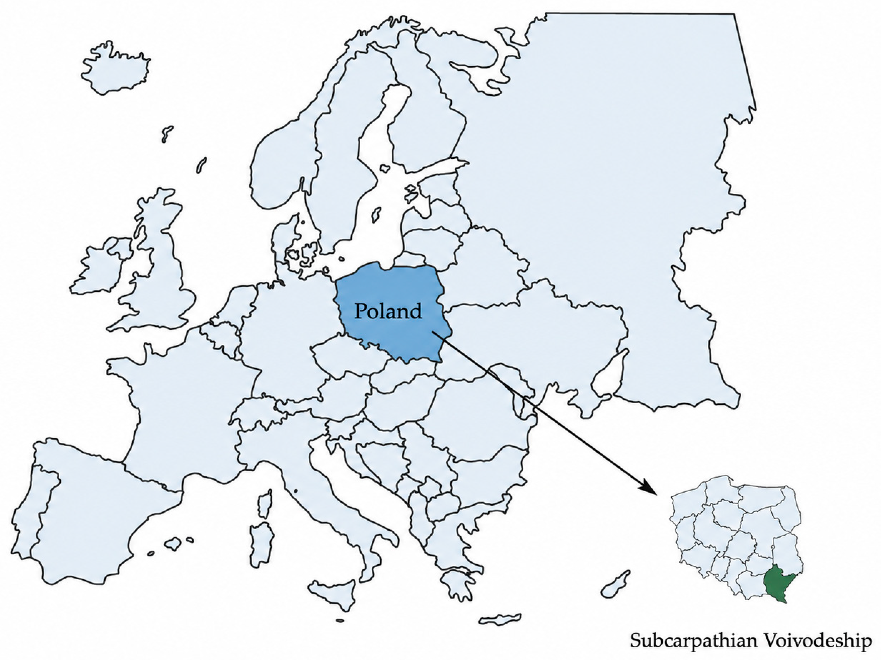
The analysis concerns an anonymised urban water distribution system in the Subcarpathian region of south-eastern Poland (Figure 1). The system is operated by a municipal waterworks company, and the analysed network length has increased by approximately 84.4% from almost 600 km in 2004 [40].

Figure 1 shows the regional setting of the study area.

3.2. Source Records

The source material comprised a database consisting of 22 annual failure registers covering the period 2004–2025 provided by the municipal waterworks company [40].

The resulting record flow is summarised in

Table 1. Record flow and outcome-specific analytical denominators.

Stage	n
Numbered source events	4885
Repair duration calculable	4859
Service-interruption status/duration calculable	4832
Explicit ‘no shut-off’	1039
All numerical zero interruptions	1044
Unique material identified	4824
Pipe function classified	4876
Unique material and pipe function	4817
Primary MCDM set	4806 in 14 groups

.

3.3. Technical Classification and Temporal Comparability

Material labels were harmonised to cast iron, steel, galvanised steel, PVC, PE and asbestos cement (AC). To align every numerator with its exposure denominator, an analytical pipe-function proxy was assigned solely from the diameter for every event and every single-diameter inventory row: service connections, distribution pipes and mains. Failure descriptions were assigned once to the mutually exclusive classes corrosion, leaky socket, loss of tightness, crack, mechanical damage and other/unclear, and the same rule was used for the all-event occurrence analysis and every outcome-specific subset. Rare technical-wear and breakage entries were included in other/unclear.

Annual total, function-specific and material–diameter lengths were available throughout 2004–2025. The same diameter boundaries were applied to the material–diameter inventory. Cross-source reconstruction identified one harmonised material for 4824 of 4885 events (98.75%); 48 remained unknown and 13 were explicitly mixed. Of all events, 4817 also had an unambiguous pipe function. The primary material–function decision matrix used the full 2004–2025 period, with numerator and exposure years aligned.

Cause-by-function occurrence analysis retained all 4885 numbered events. For each cause and pipe function, λ was calculated using Equation (1) and the 2004–2025 cumulative exposure of the corresponding functional class. Nine events without a usable diameter were retained in the all-event cause totals but were excluded from function-specific failure rates.

3.4. Variables and Descriptive Analyses

Annual and period-specific rates used corresponding annual exposure. Arithmetic means are reported with non-parametric 95% bootstrap confidence intervals; medians and interquartile ranges (IQRs) describe the strongly heaped duration data. Temporal monotonicity was assessed using Spearman’s ρ and Kendall’s τ, and Theil–Sen slopes describe annual change. Kruskal–Wallis tests compared repair and interruption distributions across pipe function, full-period material, diameter class and failure cause. Tests are global and do not imply causality. The three analysis subperiods—2004–2010, 2011–2017 and 2018–2025—divide the 22-year record into approximately equal intervals. They were defined for the revised analysis, rather than preregistered, to retain sufficient observations in each interval and limit sensitivity to single-year fluctuations. Statistical analyses were performed using STATISTICA version 13.3 (TIBCO Software Inc., Palo Alto, CA, USA).

3.5. Operational Indicators

For a material–function group g in the full 2004–2025 period, the exposure-normalised failure rate was:

$${\lambda }_g = {\displaystyle \frac{n_g}{{\sum }_{t=2004}^{2025}{L}_{g,t}}}$$

(1)

Mean repair duration and mean service-interruption duration used their own valid denominators:

$${MTTR}_g = {\displaystyle \frac{{\sum }_{i=1}^{n_{g,r}}{T}_{\mathrm{repair},g,i}}{n_{g,r}}}$$

(2)

$${SIT}_g={\displaystyle \frac{{\sum }_{i=1}^{n_{g,s}}{T}_{\mathrm{SI},g,i}}{n_{g,s}}}$$

(3)

The dependent burden indicators were retained for sensitivity analysis, not as independent primary evidence:

$${RBI}_g = {\lambda }_g\times {MTTR}_g$$

(4)

$${SIBI}_{g }={ \lambda }_g\times {SIT}_g$$

(5)

Repair-time threshold sensitivity was defined as:

$$P\left(T_{\mathrm{repair}} > \tau \right)={\displaystyle \frac{n\left(T_{\mathrm{repair}}>\tau \right)}{n_{g,r}}},\tau \in \{8 \mathrm{h},10 \mathrm{h},12 \mathrm{h}\}$$

(6)

In Equation (6), the group-specific denominator n_g,r is the number of valid repair durations rather than the occurrence count used in Equation (1). Threshold indicators were not included in the primary core model after the empirical correlation audit showed near redundancy with MTTR.

3.6. CRITIC–TOPSIS Models

Alternatives were material–function groups with at least ten events in 2004–2025. All criteria were benefit-type in the priority sense: a larger value indicated a greater need for investigation. The primary core model comprised λ, MTTR and SIT. Six structural sensitivity models were also calculated: positive-SIT core (λ, MTTR and the mean conditional on SIT > 0); threshold-augmented (core + P(T_repair > 8 h)); burden (RBI, SIBI and P(T_repair > 8 h)); full (all six); no-RBI; and no-SIBI. This design tests both interruption coding and the effect of deterministic products rather than assuming independence.

For CRITIC, each criterion was min–max-scaled. Its information content combined contrast (standard deviation σ_j) with conflict (Pearson correlation ρ_jk), and weights were normalised to sum to one:

$$C_j = {\sigma }_j\sum _{k=1}^q\left(1 - {\rho }_{jk}\right)$$

(7)

$$w_j={\displaystyle \frac{C_j}{{\sum }_{j=1}^q{C}_j}}$$

(8)

In Equations (7) and (8), q is the number of criteria and is distinct from the event count n. TOPSIS used vector normalisation and Euclidean distances $D_i^{+}$ and $D_i^{-}$ from the positive and negative ideal profiles. The complete normalisation, weighting, ideal profile and distance equations are reported in Appendix A.3. The relative priority score was:

$${CC}_i = {\displaystyle \frac{D_i^{-}}{D_i^{+}+D_i^{-}}}$$

(9)

Scores are relative to the alternatives in the decision matrix and are not probabilities, risk values or universal intervention thresholds. No arbitrary high/medium/low classes were imposed.

3.7. Uncertainty, Sensitivity and Adjusted Modelling

The core ranking was first bootstrapped 2000 times with a fixed random seed by sampling the 4806 eligible pooled events with replacement. Failure rate used all sampled events, whereas MTTR and SIT used their own sampled valid-outcome counts; a missing duration never entered a sum or denominator. Group exposure remained fixed, and CRITIC weights and TOPSIS scores were recomputed in every replicate. All 2000 replicates contained at least one valid repair and interruption value for every alternative. Reported outputs are the median and 95th percentile interval for score and rank, P(rank 1), and P(rank ≤ 3). The conventional event-level scheme treats registered events as exchangeable and conditionally independent; it does not retain within-year clustering or dependence from repeat failures of the same segment.

As a dependence sensitivity analysis, a second set of 2000 calendar-year block bootstrap replicates sampled 22 years with replacement. Every selected year contributed all of its eligible events and the corresponding annual material–function exposure; outcome-specific missingness rules were retained, and CRITIC weights and TOPSIS scores were recomputed. This preserved within-year event clustering and the coupling between annual failures and exposure. Both bootstrap analyses remain conditional on the observed material and diameter assignments and do not propagate classification or inventory error.

Sensitivity analyses varied:

• Interruption representation through positive-only SIT;
• Criterion structure;
• Repair threshold (>8, ≥8, >10 and >12 h);
• Minimum group size (10, 20, 30 and 50 events);
• The same three analysis subperiods used for descriptive comparison.

For subperiod stability, the core ranking was recomputed within 2004–2010, 2011–2017 and 2018–2025 among groups with at least ten events in all three intervals. CRITIC weights and TOPSIS normalisation were re-estimated within each subperiod; Spearman rank correlation against the full-period core ranking and maximum absolute rank change summarised agreement.

To examine whether material differences persisted after observed confounding, log repair duration was regressed on year, log diameter, material, pipe function and grouped failure causes for 4792 complete full-period events. Ordinary least squares coefficients were reported as multiplicative effects after exponentiation, with HC3 heteroscedasticity-robust confidence intervals. PE, distribution pipes and corrosion were reference categories. This model is explanatory and not a validated failure-duration predictor.

Service interruption was also analysed with a two-part adjusted model using the same covariates and reference categories. The first part used logistic regression for a recorded shut-off/restoration interval versus an explicit ‘no water shut-off’ entry; the second used HC3-robust log-linear regression among positive recorded durations. Effects are reported as odds ratios and multiplicative duration ratios, respectively. The complete-case set contained 4765 events: 3739 recorded interruptions and 1026 explicit no-shut-off entries. Of these records, 3736 had a positive duration and 1029 were non-positive; only positive durations entered the second part.

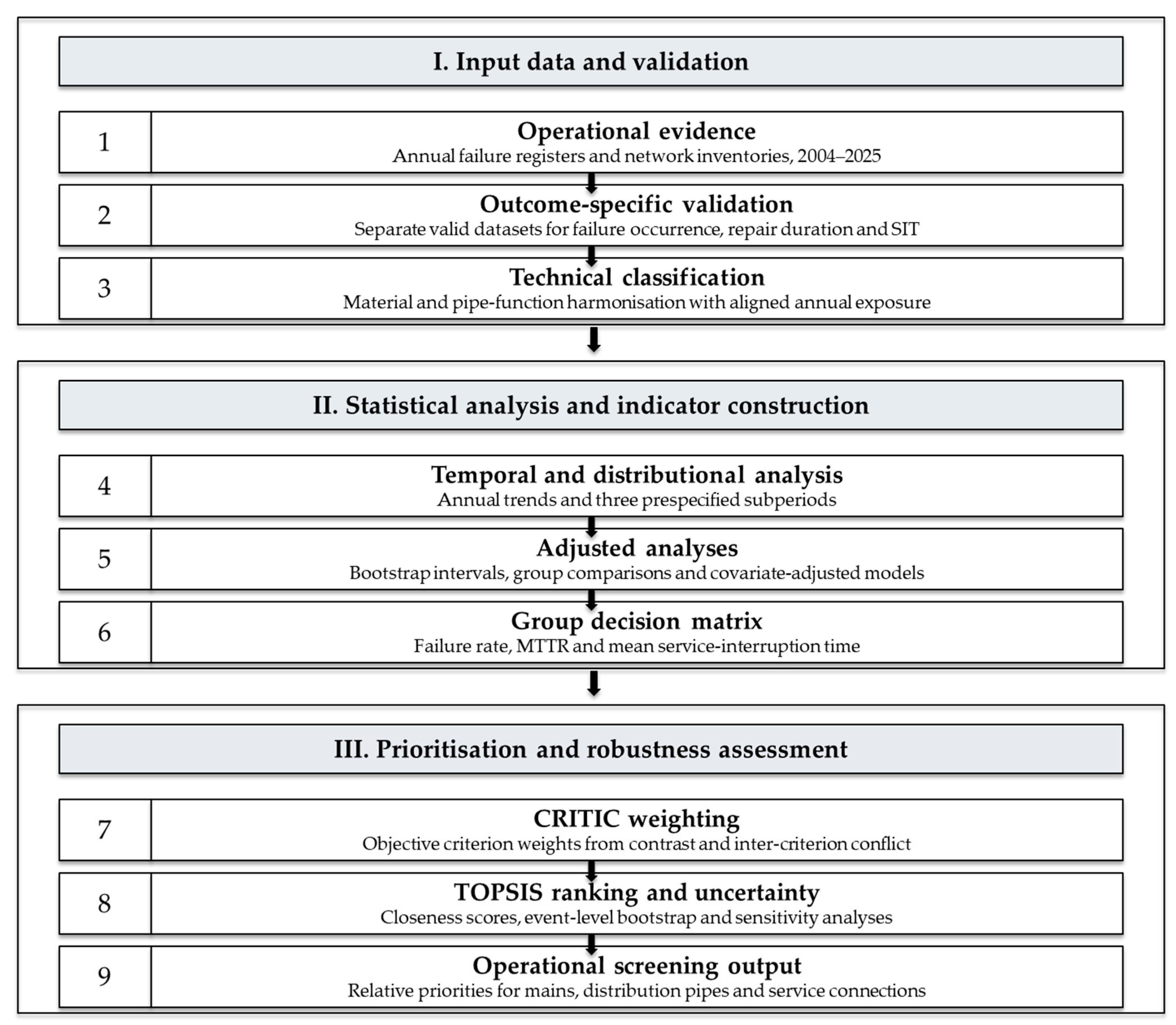
Figure 2 summarises the analytical sequence from operational evidence to screening priorities. Annual registers undergo outcome-specific validation and technical classification. Temporal and distributional analysis, adjusted models and group-indicator construction then lead to CRITIC weighting, TOPSIS ranking, event-level bootstrap uncertainty and sensitivity analyses.

4. Results

4.1. Data Completeness and Network Evolution

The source-level audit retained 4859 valid repair durations totalling 38,663.25 h and 4832 valid service-interruption values totalling 11,751.70 h. Outcome-specific denominators are used throughout, and no missing outcome is estimated.

Historical technical sources supplied a unique, source-supported material for 4824 events (98.75%); 48 records remained unknown and 13 were mixed. After also requiring a diameter-based function, 4817 events entered candidate material–function groups and 4806 in 14 groups met the primary n ≥ 10 rule.

During the analysed period, the total network length increased by 480 km. The annual event count fell from 307 to 158, so exposure-normalised failure occurrence fell more sharply, from 0.539 to 0.150 failures/(km·year). Failure rate had a strong negative trend (ρ = −0.911, p < 0.001; Theil–Sen slope: −0.016 failures/(km·year) per year, 95% CI: −0.020 to −0.013). The failure rate trend should not be interpreted as a treatment effect because network renewal, expansion and asset mix changed concurrently.

4.2. Temporal Patterns

Table 2. Subperiod comparison with outcome-specific denominators.

Subperiods	Events	Exposure (km·yr)	λ (Failures/(km·year)	nrepair	MTTR (h)	Median (IQR) Repair (h)	nSIT	Mean SIT (h)
2004–2010	1718	4444.58	0.387	1693	7.61	8.00 (2.00)	1673	2.41
2011–2017	1797	5597.72	0.321	1796	8.21	8.00 (0.00)	1791	1.68
2018–2025	1370	8015.02	0.171	1370	8.06	8.00 (0.00)	1368	3.44

compares event counts, cumulative pipe-length exposure and outcome-specific time summaries across the three analysis subperiods.

MTTR varied within a comparatively narrow range (7.61–8.21 h), and the annual MTTR trend was not significant (ρ = 0.264, p = 0.236). Mean service-interruption duration was lowest in 2011–2017 (1.68 h) and highest in 2018–2025 (3.44 h). Its annual increasing trend was statistically detectable (ρ = 0.560, p = 0.007) (Table 2). The annual mean repair duration and mean service-interruption duration for 2004–2025 are presented in

Table 3. Annual mean repair duration and mean service-interruption duration, 2004–2025.

Year	Repair Duration		Service Interruption
	Mean Repair Duration, MTTR (h)	95% Bootstrap CI (h)	Mean Service-Interruption Duration (h)	95% Bootstrap CI (h)
2004	6.75	6.39–7.11	2.99	2.68–3.34
2005	7.60	7.08–8.15	3.22	2.65–3.82
2006	7.34	7.02–7.70	1.95	1.68–2.22
2007	7.86	7.55–8.19	2.14	1.88–2.40
2008	7.73	7.52–7.95	2.35	2.16–2.54
2009	8.18	7.92–8.47	2.13	1.86–2.42
2010	8.17	7.96–8.40	2.06	1.86–2.28
2011	8.24	7.99–8.49	1.39	1.21–1.62
2012	8.21	7.93–8.49	1.40	1.25–1.54
2013	8.47	8.18–8.77	1.55	1.40–1.71
2014	8.14	7.81–8.47	1.62	1.41–1.84
2015	8.03	7.76–8.31	1.58	1.40–1.77
2016	8.02	7.73–8.33	2.36	2.13–2.63
2017	8.37	8.03–8.73	2.04	1.74–2.36
2018	8.29	7.91–8.69	2.97	2.64–3.31
2019	8.28	7.95–8.62	3.56	3.26–3.89
2020	8.09	7.67–8.52	3.49	3.22–3.76
2021	7.53	7.20–7.86	3.24	3.00–3.49
2022	8.00	7.61–8.41	3.85	3.59–4.13
2023	8.09	7.79–8.40	3.24	2.95–3.53
2024	7.85	7.53–8.17	3.42	3.17–3.70
2025	8.18	7.80–8.59	3.89	3.57–4.22

.

4.3. Repair-Time Distribution and Group Differences

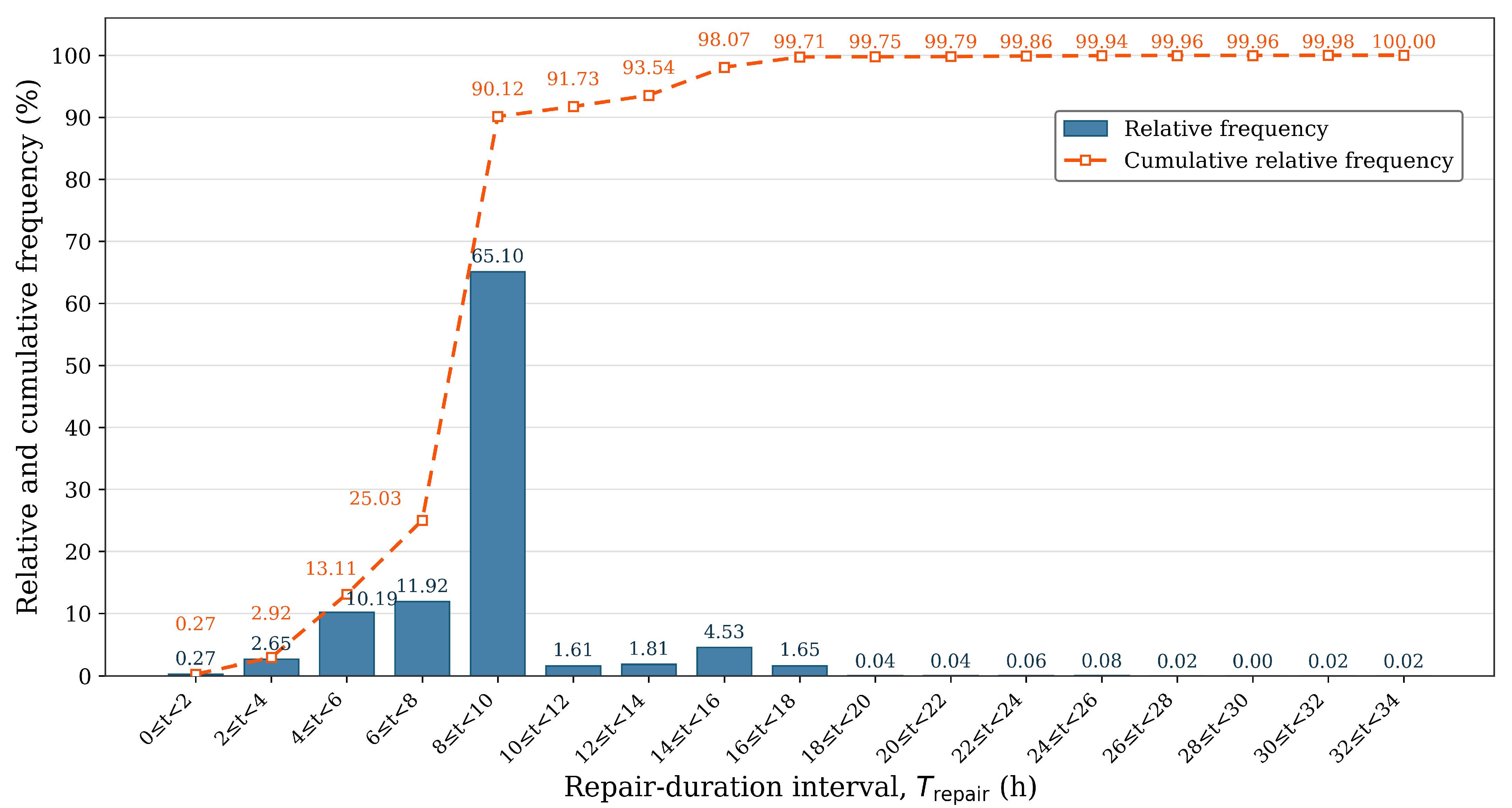
Across 4859 valid observations, mean repair duration was 7.96 h (SD 2.58 h), median was 8.00 h and IQR was 7.50–8.00 h. The distribution was dominated by recording heaping (Figure 3): 4444 values (91.5%) were whole hours and 3118 (64.2%) were exactly 8 h. Exact counts at 6, 7, 12, 16 and 24 h were 204, 220, 43, 77 and 4, respectively. Consequently, the distinction between strict and inclusive thresholds was material: 525 repairs (10.8%) were >8 h, whereas 3643 (75.0%) were ≥8 h. The proportions were 9.5% for >10 h and 7.4% for >12 h.

Table 4. Repair and service-interruption outcomes by pipe function and material (2004–2025).

Dimension	Group	Repair Duration						Service Interruption
		Nrepair	Mean (h)	SD (h)	95% CI (h)	Median (h)	Q1–Q3 (h)	nSIT	Mean (h)	SD (h)	95% CI (h)	Median (h)	Q1–Q3 (h)
Function	Mains	648	9.14	3.27	8.87–9.40	8.00	8.00–8.00	645	1.69	2.63	1.49–1.90	0.00	0.00–3.00
Function	Distribution pipes	2328	7.92	2.57	7.82–8.03	8.00	7.00–8.00	2314	2.57	2.36	2.48–2.67	2.50	1.00–3.50
Function	Service connections	1875	7.59	2.16	7.48–7.69	8.00	7.00–8.00	1865	2.52	1.94	2.44–2.61	2.00	2.00–3.00
Material	Cast iron	1868	8.17	2.79	8.04–8.30	8.00	7.50–8.00	1852	2.21	2.47	2.10–2.33	2.00	0.00–3.00
Material	Steel	1174	8.05	2.60	7.90–8.21	8.00	8.00–8.00	1170	2.19	1.92	2.08–2.30	2.00	1.00–3.00
Material	Galvanised steel	881	7.57	2.26	7.42–7.73	8.00	6.50–8.00	875	2.78	2.33	2.63–2.93	2.50	2.00–3.00
Material	PVC	305	7.72	2.44	7.44–8.00	8.00	7.00–8.00	303	3.13	2.30	2.88–3.41	3.00	2.00–4.00
Material	PE	523	7.64	2.06	7.47–7.81	8.00	8.00–8.00	524	2.61	1.84	2.46–2.76	2.50	2.00–3.50
Material	AC	47	8.47	3.16	7.63–9.33	8.00	7.00–8.00	47	3.66	2.11	3.07–4.28	3.00	2.00–5.00

reports outcome-specific sample sizes, means, uncertainty intervals and distributional summaries by pipe function and material for 2004–2025.

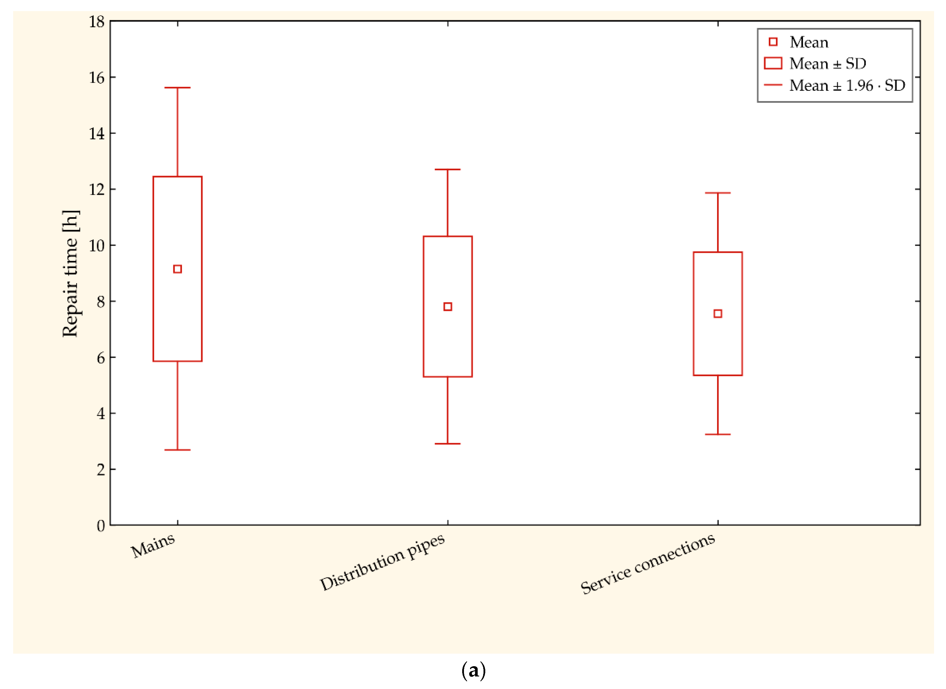
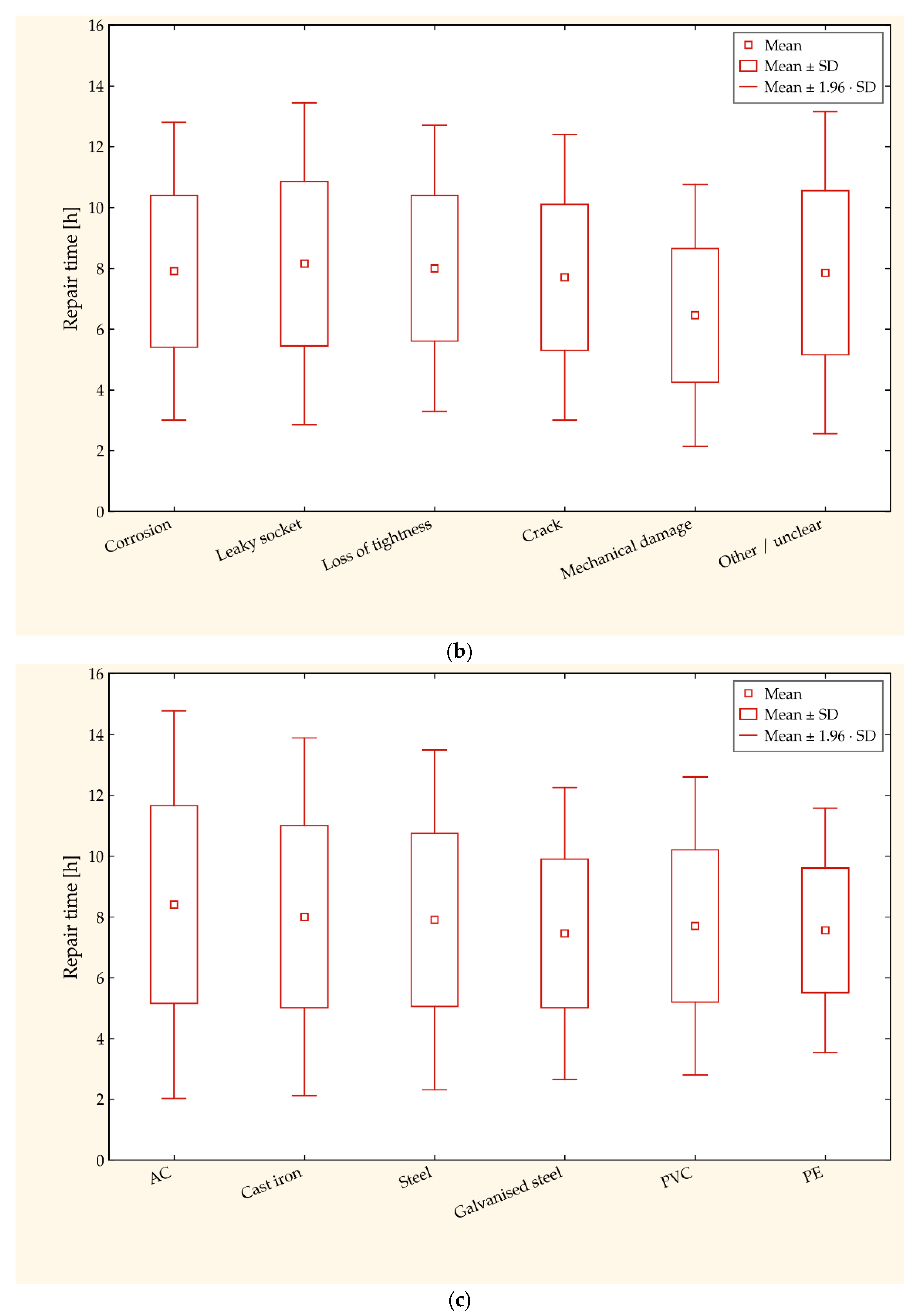
Repairs to mains had the largest unadjusted mean (9.14 h), but their mean interruption duration was the smallest (1.69 h). This divergence confirms that repair work and user-side interruption should not be merged into one time variable. AC events had the largest material-level repair mean (8.47 h; n = 47) and interruption mean (3.66 h), with wide uncertainty. Global Kruskal–Wallis tests indicated differences across function and material for both outcomes (all p < 0.001). Diameter classes also differed for both outcomes (p < 0.001), while failure-cause groups differed for repair duration (p = 0.002) and service interruption (p < 0.001; Appendix A). Given the strong heaping, statistical significance should not be confused with large operational separation. Figure 4 shows the corresponding repair-duration distributions.

Cause-specific occurrence patterns also differed by pipe function (

Table 5. Failure occurrence and exposure-normalised failure rate by cause and pipe function (2004–2025).

Failure Cause	Mains n; λ	Distribution Pipes n; λ	Service Connections n; λ	Classified Total n; Pooled λ	Unknown Function n	All Events n
Corrosion	144; 0.0758	676; 0.0715	1438; 0.2206	2258; 0.1263	3	2261
Leaky socket	420; 0.2210	674; 0.0712	15; 0.0023	1109; 0.0620	6	1115
Loss of tightness	72; 0.0379	312; 0.0330	246; 0.0377	630; 0.0352	0	630
Crack	8; 0.0042	144; 0.0152	107; 0.0164	259; 0.0145	0	259
Mechanical damage	1; 0.0005	12; 0.0013	8; 0.0012	21; 0.0012	0	21
Other/unclear	11; 0.0058	523; 0.0553	65; 0.0100	599; 0.0335	0	599
Total	656; 0.3453	2341; 0.2475	1879; 0.2882	4876; 0.2727	9	4885

). Leaky sockets dominated main exposure (420 failures; 0.2210 failures/(km·year)), whereas corrosion dominated service connections (1438; 0.2206 failures/(km·year)). In distribution pipes, corrosion (676; 0.0715 failures/(km·year)) and leaky sockets (674; 0.0712 failures/(km·year)) were nearly equal. Across all causes, the pooled failure rate was highest for mains (0.3453 failures/(km·year)), followed by service connections (0.2882 failures/(km·year)) and distribution pipes (0.2475 failures/(km·year)).

4.4. Adjusted Repair and Interruption Models

The complete covariate-adjusted repair-duration model is reported in

Table 6. Complete adjusted log repair-duration model (n = 4792).

Term	Multiplicative Effect	95% HC3 CI	p
Year (per year)	1.006	1.005–1.008	<0.001
log(diameter/100 mm)	1.072	1.038–1.107	<0.001
Material: PVC	1.024	0.979–1.071	0.299
Material: Cast iron	1.112	1.056–1.170	<0.001
Material: Steel	1.087	1.023–1.155	0.007
Material: Galvanised steel	1.061	0.998–1.129	0.057
Material: AC	1.145	1.025–1.278	0.017
Function: Service connections	1.046	1.001–1.091	0.043
Function: Mains	1.063	1.014–1.115	0.011
Cause: Leaky socket	0.944	0.904–0.985	0.008
Cause: Loss of tightness	1.036	0.978–1.096	0.229
Cause: Crack	1.011	0.951–1.074	0.729
Cause: Other/unclear	0.959	0.914–1.006	0.084

.

After adjustment, cast iron was associated with an estimated 11.2% longer repair duration than PE (95% CI: 5.6–17.0%; p < 0.001), steel with an 8.7% longer duration (95% CI: 2.3–15.5%; p = 0.007) and AC with an 14.5% longer duration (95% CI: 2.5–27.8%; p = 0.017). PVC was not statistically distinguishable from PE, and galvanised steel narrowly missed p < 0.05 (p = 0.057). A one-unit increase in log(diameter/100 mm) was associated with a 7.2% longer repair; repairs to service connections and mains were 4.6% and 6.3% longer than repairs to distribution pipes after adjustment. The small R² (0.053) indicates that the measured covariates explain little individual-duration variation; it does not identify the source of the unexplained remainder or validate material as a stand-alone causal decision rule.

The two-part interruption model produced different occurrence and duration patterns (

Table A3. Complete adjusted two-part model for recorded service interruption.

Model Part	Term	Effect	95% HC3 CI	p
Occurrence OR	Year (per year)	1.107	1.092–1.123	<0.001
Occurrence OR	log(diameter/100 mm)	0.469	0.358–0.616	<0.001
Occurrence OR	Material: PVC	2.476	1.353–4.531	0.003
Occurrence OR	Material: Cast iron	1.650	0.980–2.778	0.060
Occurrence OR	Material: Steel	0.931	0.524–1.655	0.807
Occurrence OR	Material: Galvanised steel	1.179	0.640–2.173	0.598
Occurrence OR	Material: AC	1.682	0.386–7.330	0.489
Occurrence OR	Function: Service connections	0.792	0.546–1.148	0.219
Occurrence OR	Function: Mains	0.898	0.615–1.313	0.581
Occurrence OR	Cause: Leaky socket	0.203	0.140–0.296	<0.001
Occurrence OR	Cause: Loss of tightness	0.882	0.520–1.499	0.643
Occurrence OR	Cause: Crack	2.823	1.406–5.668	0.004
Occurrence OR	Cause: Other/unclear	3.483	2.115–5.738	<0.001
Positive-duration ratio	Year (per year)	1.009	1.006–1.012	<0.001
Positive-duration ratio	log(diameter/100 mm)	1.153	1.087–1.223	<0.001
Positive-duration ratio	Material: PVC	1.071	0.993–1.154	0.075
Positive-duration ratio	Material: Cast iron	1.118	1.018–1.228	0.020
Positive-duration ratio	Material: Steel	0.981	0.882–1.089	0.714
Positive-duration ratio	Material: Galvanised steel	1.174	1.054–1.308	0.004
Positive-duration ratio	Material: AC	1.302	1.098–1.544	0.002
Positive-duration ratio	Function: Service connections	1.007	0.935–1.084	0.853
Positive-duration ratio	Function: Mains	0.905	0.810–1.011	0.078
Positive-duration ratio	Cause: Leaky socket	0.891	0.818–0.971	0.008
Positive-duration ratio	Cause: Loss of tightness	1.063	0.957–1.181	0.256
Positive-duration ratio	Cause: Crack	1.027	0.928–1.137	0.603
Positive-duration ratio	Cause: Other/unclear	1.052	0.974–1.136	0.200

). After adjustment, each later calendar year was associated with greater odds of a recorded interruption rather than an explicit no-shut-off entry (OR: 1.107, 95% CI: 1.092–1.123) and a 0.9% longer positive duration (ratio: 1.009, 95% CI: 1.006–1.012). Larger diameter was associated with lower odds of a recorded interruption (OR: 0.469 per log-diameter unit) but longer duration when a positive interruption occurred (ratio: 1.153). Relative to PE, PVC had higher odds of a recorded interruption (OR: 2.476), whereas cast iron, galvanised steel and AC had 11.8%, 17.4% and 30.2% longer positive durations. These associations are descriptive: the positive-duration R² was only 0.057.

4.5. Criterion Dependence and Point Rankings

Table 7. Full-period decision matrix and core CRITIC–TOPSIS results (2004–2025).

Group	n (all/r/SIT)	Exposure (km·yr)	λ km−1·yr−1	MTTR (h)	SIT (h)	P(>8 h)	RBI h/(km·yr)	SIBI h/(km·yr)	Core CC	Rank
S–galvanised steel	849 (848/842)	483.12	1.757	7.58	2.77	0.071	13.32	4.86	0.819	1
DP–steel	460 (459/459)	293.17	1.569	7.92	2.35	0.107	12.43	3.69	0.757	2
DP–AC	44 (44/44)	35.86	1.227	8.50	3.86	0.227	10.43	4.74	0.708	3
DP–galvanised steel	29 (29/29)	22.90	1.266	7.14	3.21	0.103	9.04	4.06	0.683	4
DP–cast iron	1381 (1371/1357)	1696.08	0.814	7.92	2.43	0.112	6.45	1.98	0.437	5
S–cast iron	29 (27/26)	44.22	0.656	7.57	2.19	0.074	4.97	1.44	0.343	6
M–cast iron	472 (466/465)	802.56	0.588	8.93	1.59	0.217	5.25	0.94	0.305	7
DP–PVC	219 (219/218)	3646.05	0.060	7.76	3.26	0.087	0.47	0.20	0.207	8
M–PE	37 (37/37)	403.48	0.092	9.05	2.68	0.243	0.83	0.25	0.177	9
M–steel	130 (128/126)	581.79	0.223	9.84	1.66	0.328	2.20	0.37	0.176	10
DP–PE	169 (168/169)	3736.68	0.045	7.94	2.83	0.101	0.36	0.13	0.164	11
S–PVC	80 (80/79)	533.80	0.150	7.47	2.69	0.063	1.12	0.40	0.159	12
S–PE	318 (318/318)	2073.26	0.153	7.32	2.49	0.031	1.12	0.38	0.136	13
S–steel	589 (587/585)	3339.37	0.176	7.76	2.18	0.053	1.37	0.38	0.115	14

presents the full-period group decision matrix and the resulting three-criterion core ranking.

Within the core model, CRITIC assigned weights of 0.347 to failure rate, 0.366 to MTTR and 0.287 to SIT. Galvanised-steel service connections ranked first (CC = 0.819), followed by steel distribution pipes (0.757) and AC distribution pipes (0.708). The first group combined the largest length-normalised failure rate (1.757 failures/(km·year)) with moderate mean times. Its point rank was driven mainly by 849 repeated events over 483.12 km·years of exposure, not by the longest individual repairs; the segments within this class should therefore be checked for event concentration and coding consistency before renewal action.

The dependence audit was decisive. RBI correlated 0.996 with failure rate, SIBI correlated 0.962 with failure rate, and RBI and SIBI correlated 0.960. MTTR and P(T_repair > 8 h) correlated 0.944 because of the heaped repair distribution. Accordingly, the threshold and product criteria were not treated as additional independent evidence in the core model.

Table 8. CRITIC diagnostics for the three-criterion core model.

Criterion	Scaled σj	Conflict Σ(1 − ρjk)	Information Cj	Point Weight	Bootstrap Median Weight (95% Interval)
λ	0.340	1.985	0.674	0.347	0.355 (0.314–0.407)
MTTR	0.272	2.611	0.710	0.366	0.356 (0.311–0.403)
SIT	0.258	2.157	0.557	0.287	0.287 (0.247–0.329)

reports the contrast, conflict, information and point and bootstrap weight components of the core CRITIC model.

Table 9. Criterion correlations.

Criterion	λ			MTTR		SIT			P(T > 8)		RBI		SIBI
λ	1.00			−0.22		0.23			−0.06		1.00		0.96
MTTR	−0.22			1.00		−0.39			0.94		−0.16		−0.23
SIT	0.23			−0.39		1.00			−0.19		0.22		0.45
P(T > 8)	−0.06			0.94		−0.19			1.00		−0.00		−0.03
RBI	1.00			−0.16		0.22			−0.00		1.00		0.96
SIBI	0.96			−0.23		0.45			−0.03		0.96		1.00
where
Value		1.00	0.75		0.50		0.25	0.00		−0.25	−0.50	−0.75		−1.00
Colour

and

Table 10. Ranks under alternative criterion structures.

Pipe Group			Core		Positive-SIT Core			Threshold-Augmented			Burden			Full			No RBI			No SIBI
S–galvanised steel			1		1			2			3			2			2			2
DP–steel			2		2			3			4			3			3			3
DP-AC			3		4			1			1			1			1			1
DP–galvanised steel			4		3			4			5			4			4			4
DP–cast iron			5		5			5			8			7			6			7
S–cast iron			6		6			9			9			9			9			9
M–cast iron			7		7			7			6			6			7			6
DP-PVC			8		10			10			11			10			10			10
M-PE			9		9			8			7			8			8			8
M–steel			10		8			6			2			5			5			5
DP-PE			11		13			11			10			11			11			11
S-PVC			12		14			12			12			12			12			12
S-PE			13		12			13			14			13			13			13
S–steel			14		11			14			13			14			14			14
where
Rank	1	2		3		4	5		6	7		8	9		10	11		12	13		14
Colour

show the complete criterion-correlation matrix and the rank changes produced by alternative criterion structures.

4.6. Bootstrap Uncertainty and Sensitivity

Table 11. Core-model bootstrap uncertainty (2000 event-level replicates).

Group	Observed CC	Bootstrap Median CC	95% Bootstrap CC	Median Rank (95% Interval)	P(Rank 1)	P(Top 3)
S–galvanised steel	0.819	0.819	0.770–0.866	1.0 (1.0–2.0)	0.800	1.000
DP–steel	0.757	0.755	0.691–0.814	2.0 (2.0–4.0)	0.001	0.922
DP–AC	0.708	0.700	0.528–0.891	3.0 (1.0–4.0)	0.138	0.603
DP–galvanised steel	0.683	0.679	0.467–0.843	4.0 (1.0–4.0)	0.062	0.475
DP–cast iron	0.437	0.438	0.403–0.475	5.0 (5.0–6.0)	–	–
S–cast iron	0.343	0.344	0.221–0.478	6.0 (5.0–8.0)	–	0.001
M–cast iron	0.305	0.306	0.273–0.341	7.0 (6.0–7.0)	–	–
DP–PVC	0.207	0.212	0.157–0.266	8.0 (8.0–10.0)	–	–
M–PE	0.177	0.185	0.110–0.254	10.0 (8.0–14.0)	–	–
M–steel	0.176	0.178	0.149–0.209	10.0 (8.0–13.0)	–	–
DP–PE	0.164	0.169	0.118–0.229	11.0 (8.0–13.0)	–	–
S–PVC	0.159	0.165	0.117–0.223	11.0 (9.0–13.0)	–	–
S–PE	0.136	0.142	0.106–0.186	13.0 (11.0–14.0)	–	–
S–steel	0.115	0.123	0.095–0.161	14.0 (13.0–14.0)	–	–

Where (–) indicates that the corresponding ranking outcome was not observed in any replicate.

summarises score and rank uncertainty for every alternative across the 2000 event-level bootstrap replicates.

Galvanised-steel service connections led the point ranking and had a bootstrap score interval of 0.770–0.866, rank interval of 1–2, P(rank 1) = 0.800 and P(top 3) = 1.000 (Table 11). Steel distribution pipes had P(top 3) = 0.922 and a rank interval of 2–4. AC distribution pipes had P(rank 1) = 0.138, P(top 3) = 0.603 and a rank interval of 1–4; galvanised-steel distribution pipes had corresponding probabilities of 0.062 and 0.475. Thus, sampling variation alone does not make first place certain. These probabilities are conditional on the audited classification and fixed annual exposure, and are neither hydraulic-consequence probabilities nor probabilities of future failure.

The calendar-year block bootstrap retained galvanised-steel service connections as the leading group in 68.4% of replicates and in the top three in 100.0%; their median CC was 0.810 (95% interval: 0.687–0.867) and median rank was 1 (95% interval: 1–3). Corresponding P(top 3) values were 0.872 for steel distribution pipes, 0.686 for AC distribution pipes and 0.442 for galvanised-steel distribution pipes. The lower P(rank 1) than in the event-level bootstrap (0.684 versus 0.800) shows that annual clustering adds uncertainty without changing the leading group.

Table 12. Structural, threshold, minimum-representation and subperiod sensitivity.

Sensitivity	Specification	Top Group	Rank Correlation	Maximum Change/Note
Criterion structure	Core	S–galvanised steel	1.000	0
Criterion structure	Positive-SIT core	S–galvanised steel	0.938	3
Criterion structure	Threshold-augmented	DP–AC	0.921	4
Criterion structure	Burden	DP–AC	0.754	8
Criterion structure	Full	DP–AC	0.890	5
Criterion structure	No RBI	DP–AC	0.899	5
Criterion structure	No SIBI	DP–AC	0.890	5
Repair threshold	>8 h	DP–AC	1.000	0
Repair threshold	≥8 h	S–galvanised steel	0.921	4
Repair threshold	>10 h	DP–AC	0.982	2
Repair threshold	>12 h	DP–AC	0.982	2
Minimum group n	n ≥ 10	S–galvanised steel	—	14 alternatives
Minimum group n	n ≥ 20	S–galvanised steel	—	14 alternatives
Minimum group n	n ≥ 30	S–galvanised steel	—	12 alternatives
Minimum group n	n ≥ 50	S–galvanised steel	—	10 alternatives
Subperiod	2004–2010	S–galvanised steel	0.818	4
Subperiod	2011–2017	DP–AC	0.727	5
Subperiod	2018–2025	S–galvanised steel	0.927	3

compares the structural, threshold, minimum-representation and subperiod sensitivity analyses.

Threshold correlations are strictly against >8 h within the threshold-augmented model. Subperiod correlations are against the full-period core ranking among the 11 groups with at least ten events in all three subperiods. Criterion structure materially affected the result. Replacing SIT with the mean conditional on a positive interruption retained galvanised-steel service connections as the leader (Spearman ρ = 0.938 versus the core; maximum rank change = 3). By contrast, the threshold-augmented, burden, full, no-RBI and no-SIBI models all ranked AC distribution pipes first; their rank correlations with the core model were 0.921, 0.754, 0.890, 0.899 and 0.890, with maximum individual changes of four to eight ranks. Under threshold augmentation, strict > 8 h, >10 h and >12 h definitions selected AC distribution pipes, whereas inclusive ≥8 h selected galvanised-steel service connections. Minimum group sizes from n ≥ 10 through n ≥ 50 retained galvanised-steel service connections as the core-model leader. Structural and representation sensitivities must therefore accompany, not merely decorate, the point ranking.

Temporal stability was assessed using the same three analysis subperiods as Table 2. Eleven groups had at least ten events in all three intervals. Galvanised-steel service connections ranked first in 2004–2010 and 2018–2025, whereas AC distribution pipes ranked first in 2011–2017. Rank correlations with the full-period core ranking were 0.818, 0.727 and 0.927, with maximum changes of four, five and three ranks, respectively. This supports periodic recalculation and shows that leader stability is not uniform across the full observation period.

5. Discussion

5.1. Interpretation of the Ranking

With one diameter-based function rule applied to both event counts and annual exposure, and dependent criteria excluded from the primary model, galvanised-steel service connections have the highest point priority, representing 849 events and 483.12 km·years of exposed stock. They remained first at minimum group sizes through n ≥ 50 and in the positive-only SIT model, but not in every subperiod, bootstrap resample or structural model.

Steel distribution pipes ranked second in the full-period point model, with a bootstrap rank interval of 2–4 and P(top 3) = 0.922. AC distribution pipes illustrated a different uncertainty pattern: their rank interval of 1–4 and P(top 3) = 0.603 arose from only 44 observations on 35.86 km·years of exposure. They led all product-containing structures and the strict >8, >10 and >12 h threshold variants; the inclusive ≥8 h variant retained galvanised-steel service connections. AC distribution pipes ranked fourth in the positive-only SIT model, showing that a small group can be influential when its repair and interruption means are high.

The observed rates can also be compared with the literature-based reference criteria. Kwietniewski proposed a general three-class classification in which λ ≤ 0.10 failures/(km·year) denotes a low failure rate and high reliability, 0.10 < λ ≤ 0.50 a moderate failure rate and reliability, and λ > 0.50 a high failure rate and low reliability [41]. On this general scale, the pooled function-classified rate of 0.2727 failures/(km·year) was moderate. Rak proposed function-specific reference values of λ ≤ 0.30 failures/(km·year) for mains, λ ≤ 0.50 for distribution pipes and λ ≤ 1.00 for service connections [42]. The reported function-specific values represent pooled exposure-weighted failure rates over the entire 2004–2025 observation period. On this full-period basis, the main rate (0.3453 failures/(km·year)) exceeded its reference value, whereas the distribution-pipe (0.2475 failures/(km·year)) and service-connection (0.2882 failures/(km·year)) rates remained below theirs. Considering the most recent annual rates, all three pipe-function classes satisfy the corresponding reference criteria, indicating an improvement relative to the long-term pooled assessment.

5.2. Relation to Existing Rehabilitation Research

The results complement rather than replace risk-based criticality methods. Prior studies identify importance through pressure loss and supply shortage [9,10], as well as topology and resilience [11,12]. The present indicators instead measure observed operational recurrence and time. A low-rate main may still be hydraulically critical, while a high-rate service class can dominate work orders without threatening system-wide supply. In future work, combining the two layers is therefore preferable: operational screening identifies where recurring burdens occur, while hydraulic and customer analyses determine their consequences.

The adjusted model is consistent with earlier local repair-time work identifying material, diameter, damage type, pavement, crew capacity and concurrent failures as plausible determinants [18]. Broader reviews show why heterogeneous records and omitted operational factors constrain event-level explanation [6,7]. The low R² shows only that the measured covariates explain little variance; it does not establish which omitted factor accounts for the remainder. Site access, pavement, excavation depth, fittings, isolation, crew availability and concurrent failures should be recorded if repair-duration prediction is a future objective.

The criterion-dependence result has wider MCDA relevance. Objective weighting does not make deterministically derived criteria independent. CRITIC down-weights some redundancy through correlation, but it cannot prevent a concept from entering the decision geometry twice. The core-versus-burden comparison therefore belongs before, not after, interpretation. The rank changes observed here are consistent with calls to analyse TOPSIS robustness and uncertainty explicitly [30].

The practical consequences also span three dimensions that cannot be collapsed into CC. Technically, recurring repairs consume crews, fittings and isolation capacity. Environmentally, excavation, leakage, flushing and replacement materials can create water, energy and material burdens. Socioeconomically, interruption duration interacts with the number and vulnerability of users, critical facilities, traffic disruption and direct cost. The present register observes only part of the technical dimension and one duration component of service consequence, so these wider effects must be added during segment-level appraisal rather than inferred from the group rank.

5.3. Operational Use

The output should be embedded in a staged utility workflow:

• Recalculate annual and rolling material–function indicators with outcome-specific denominators and automated data-quality flags.
• Review the leading groups for denominator anomalies, repeated addresses, coding errors and concentration in a small number of segments.
• For verified segments, add age, condition, break history, pressure, valve isolation, customers and critical facilities affected, water not supplied and traffic/access consequences.
• Compare feasible interventions using life-cycle cost, hydraulic benefit, regulatory constraints and coordinated street works.
• Record the decision and subsequent performance so that the screening model can be recalibrated.

The sequence is consistent with rehabilitation sorting and method comparison studies [19,20,21] and with broader asset-management guidance and risk models [22,23,24]. It also prevents a group-level closeness coefficient from being mistaken for a segment-level investment case.

5.4. Resource-Management Implications and Transferability

The proposed framework can be interpreted as a resource-allocation screening tool. The exposure-normalised failure rate represents the recurrent demand generated by a pipe group relative to the amount of infrastructure operated. Mean repair duration reflects the time for which maintenance capacity, equipment and associated operational resources remain committed to an intervention, whereas service-interruption duration reflects a temporary reduction in the accessibility of supplied drinking water to users. RBI and SIBI provide complementary exposure-normalised measures of the accumulated repair and service-interruption burdens. These indicators therefore connect asset deterioration with the management of both infrastructure resources and water-service accessibility.

At the portfolio level, the ranking can help utilities concentrate inspection, preventive maintenance and renewal assessment on pipe groups generating recurrent operational burdens rather than applying uniform replacement strategies across the network. Such targeting can support more efficient use of limited maintenance and capital budgets and may help avoid premature replacement of lower-burden infrastructure.

The numerical ranking obtained for the analysed system is site-specific, but the analytical workflow is transferable. Its minimum data requirements are routinely recorded failure information, pipe classification or diameter, repair duration, service-interruption status or duration, and corresponding network-length exposure. Other utilities can therefore reproduce the procedure using locally defined pipe groups, exposure data and operational or regulatory thresholds. In this sense, the principal generalisable contribution is not the ranking of individual pipe groups in the case-study network, but a reproducible approach for converting long-term operational records into an uncertainty-aware resource-management screening tool.

5.5. Limitations

The study concerns one city and a utility-specific recording process; numerical priorities are not transferable. Although 4824 events received a unique source-supported material, 48 remained unknown and 13 were explicitly mixed; residual linkage error cannot be excluded despite retained traceability and verification rules. Exact 8 h and whole-hour heaping suggests scheduled or rounded recording; threshold results are therefore sensitivity evidence, not natural risk boundaries.

The analytical pipe-function proxy is based solely on diameter; it may misclassify assets whose hydraulic or utility role differs from their diameter-defined class. Mean interruption duration does not quantify customers affected, vulnerable users, critical facilities, water not supplied, pressure deficit or alternative supply. Group exposure does not capture entry and retirement dates more finely than annual inventories. The pooled event-level bootstrap assumes exchangeable, conditionally independent records. The calendar-year block bootstrap addresses within-year clustering and annual exposure coupling, but it treats years as exchangeable and cannot model repeat-section dependence without stable segment identifiers. Bootstrap probabilities and subperiod ranks are therefore conditional on observed classification and exposure.

6. Conclusions

• The audited 2004–2025 record retained 4885 events, with separate valid denominators for repair (4859), service interruption (4832) and material (4824). Network length rose by 480 km, while annual failure rate fell from 0.539 to 0.150 failures/(km·year). Annual MTTR showed no significant monotonic trend (ρ = 0.264; p = 0.236), whereas mean SIT increased over time (ρ = 0.560; p = 0.007) and was highest in 2018–2025 (3.44 h). Because network configuration changed, this was an operational signal rather than proof of deteriorating customer service.
• Repair time was strongly heaped: 91.5% of values were whole hours and 64.2% equalled 8 h. The sharp contrast between >8 h (10.8%) and ≥8 h (75.0%) means that repair-threshold results should be treated as sensitivity evidence rather than a natural risk boundary.
• The primary ranking used only failure rate, MTTR and SIT. Galvanised-steel service connections ranked first (CC = 0.819), with P(rank 1) = 0.800 in the event-level bootstrap and 0.684 in the calendar-year block bootstrap; they remained in the block bootstrap top three in every replicate. They also led all minimum-size variants and the positive-only SIT model, but not every subperiod. AC distribution pipes led all product-containing structures and the strict >8, >10 and >12 h threshold variants, whereas the inclusive ≥8 h variant retained galvanised-steel service connections; derived RBI and SIBI should not be added to their own components as independent evidence.
• The result is a relative group-level screening signal, not a renewal prescription. Segment selection still requires hydraulic consequence, users and critical facilities affected, age, condition, isolation, access and life-cycle cost; environmental and socioeconomic benefits can be evaluated only after those dimensions are added. Cause-specific failure rates further support differentiated maintenance: leaky-socket failures dominate mains, corrosion dominates service connections, and the two mechanisms are nearly equal in distribution pipes.
• Beyond the local ranking, this study provides a transferable workflow linking failure occurrence, maintenance burden and water-service accessibility with infrastructure resource allocation. The approach can support utilities in directing limited inspection, repair and renewal resources toward pipe groups generating recurrent operational burdens, while subsequent segment-level decisions should incorporate hydraulic consequences, customers affected, condition, life-cycle cost and, where available, water-loss, energy and environmental indicators.

References

1. ISO 24512:2024; Guidelines for the Management of Drinking Water Utilities and for the Assessment of Drinking Water Services. International Organization for Standardization: Geneva, Switzerland, 2024.
2. Alegre, H.; Baptista, J.M.; Cabrera, E.; Cubillo, F.; Duarte, P.; Hirner, W.; Merkel, W.; Parena, R. Performance Indicators for Water Supply Services, 3rd ed.; IWA Publishing: London, UK, 2016. [Google Scholar]
3. Taiwo, R.; Shaban, I.A.; Zayed, T. Development of sustainable water infrastructure: A proper understanding of water pipe failure. J. Clean. Prod. 2023, 398, 136653. [Google Scholar] [CrossRef] [Scilit]
4. Scheidegger, A.; Leitão, J.P.; Scholten, L. Statistical failure models for water distribution pipes—A review from a unified perspective. Water Res. 2015, 83, 237–247. [Google Scholar] [CrossRef] [Scilit] [PubMed]
5. Barton, N.A.; Farewell, T.S.; Hallett, S.H.; Acland, T.F. Improving pipe failure predictions: Factors affecting pipe failure in drinking water networks. Water Res. 2019, 164, 114926. [Google Scholar] [CrossRef] [Scilit] [PubMed]
6. Dawood, T.; Elwakil, E.; Novoa, H.M.; Delgado, J.F.G. Water pipe failure prediction and risk models: State-of-the-art review. Can. J. Civ. Eng. 2020, 47, 1117–1127. [Google Scholar] [CrossRef] [Scilit]
7. Shaban, I.A.; Eltoukhy, A.E.E.; Zayed, T. Systematic and scientometric analyses of predictors for modelling water pipes deterioration. Autom. Constr. 2023, 149, 104710. [Google Scholar] [CrossRef] [Scilit]
8. Muddassir, M.; Zayed, T.; Taiwo, R.; Ben Seghier, M.E.A. Advancing the analysis of water pipe failures: A probabilistic framework for identifying significant factors. Sci. Rep. 2024, 14, 19218. [Google Scholar] [CrossRef] [Scilit] [PubMed]
9. Raspati, G.S.; Bruaset, S.; Bosco, C.; Mushom, L.; Johannessen, B.; Ugarelli, R. A risk-based approach in rehabilitation of water distribution networks. Int. J. Environ. Res. Public Health 2022, 19, 1594. [Google Scholar] [CrossRef] [Scilit] [PubMed]
10. Prasad, R.K. Identification of critical pipes for water distribution network rehabilitation. Water Resour. Manag. 2021, 35, 5187–5204. [Google Scholar] [CrossRef] [Scilit]
11. Pagano, A.; Giordano, R.; Portoghese, I. A pipe ranking method for water distribution network resilience assessment based on graph-theory metrics aggregated through Bayesian belief networks. Water Resour. Manag. 2022, 36, 5091–5106. [Google Scholar] [CrossRef] [Scilit]
12. Puleo, D.; Sinagra, M.; Picone, C.; Tucciarelli, T. Criticality assessment of pipes in water distribution networks based on the minimum pressure criterion. Water 2025, 17, 3185. [Google Scholar] [CrossRef] [Scilit]
13. Xing, J.; Zayed, T.; Ma, S.; Shao, Y. Predicting the time of supply interruption due to the repair of failed water pipes. Expert Syst. Appl. 2026, 305, 130930. [Google Scholar] [CrossRef] [Scilit]
14. Tchórzewska-Cieślak, B.; Rak, J.; Pietrucha-Urbanik, K.; Piegdoń, I.; Boryczko, K.; Szpak, D.; Żywiec, J. Water Supply Safety Assessment Considering the Water Supply System Resilience. Desalin. Water Treat. 2023, 288, 26–36. [Google Scholar] [CrossRef] [Scilit]
15. Łój-Pilch, M.; Zakrzewska, A. Impact of monitoring on the mean time to repair of the water supply network. E3S Web Conf. 2018, 44, 00101. [Google Scholar] [CrossRef] [Scilit]
16. Rak, J.R.; Tchórzewska-Cieślak, B.; Pietrucha-Urbanik, K. A hazard assessment method for waterworks systems operating in self-government units. Int. J. Environ. Res. Public Health 2019, 16, 767. [Google Scholar] [CrossRef] [Scilit] [PubMed]
17. Pietrucha, K. Analiza czasu odnowy i naprawy podsystemu dystrybucji wody dla miasta Rzeszowa [Analysis of restoration and repair time of the water distribution subsystem for the city of Rzeszów]. Instal 2008, 10, 113–115. [Google Scholar]
18. Iwanejko, R.; Bajer, J. Podstawy teoretyczne metody szacowania ryzyka związanego z czasem usuwania awarii sieci wodociągowej [Theoretical Foundations of a Method for Estimating Risk Related to Water-Supply Network Failure Repair Time]. Czas. Tech. Śr. 2011, 108, 75–83. [Google Scholar]
19. Caetano, J.; Carriço, N.; Covas, D. Lessons learnt from the application of MCDA sorting methods to pipe network rehabilitation prioritization. Water 2022, 14, 736. [Google Scholar] [CrossRef] [Scilit]
20. Tscheikner-Gratl, F.; Egger, P.; Rauch, W.; Kleidorfer, M. Comparison of multi-criteria decision support methods for integrated rehabilitation prioritization. Water 2017, 9, 68. [Google Scholar] [CrossRef] [Scilit]
21. Așchilean, I.; Giurca, I. Choosing a water distribution pipe rehabilitation solution using the analytical network process method. Water 2018, 10, 484. [Google Scholar] [CrossRef] [Scilit]
22. American Water Works Association. M28 Rehabilitation of Water Mains, 3rd ed.; AWWA: Denver, CO, USA, 2014. [Google Scholar]
23. Alegre, H.; Coelho, S.T.; Covas, D.; Almeida, M.C.; Cardoso, M.A. A utility-tailored methodology for integrated asset management of urban water infrastructure. Water Sci. Technol. Water Supply 2013, 13, 1444–1451. [Google Scholar] [CrossRef] [Scilit]
24. Salehi, S.; Salamati Nia, S.P. A qualitative-risk-based model to assess group decisions for planning the maintenance-renewal works of water pipelines with unreliable operational data. Water Resour. Manag. 2024, 38, 3153–3177. [Google Scholar] [CrossRef] [Scilit]
25. Chen, C.-T. Extensions of the TOPSIS for group decision-making under fuzzy environment. Fuzzy Sets Syst. 2000, 114, 1–9. [Google Scholar] [CrossRef] [Scilit]
26. Onu, U.P.; Xie, Q.; Xu, L. A fuzzy TOPSIS model framework for ranking sustainable water supply alternatives. Water Resour. Manag. 2017, 31, 2579–2593. [Google Scholar] [CrossRef] [Scilit]
27. Diakoulaki, D.; Mavrotas, G.; Papayannakis, L. Determining objective weights in multiple criteria problems: The CRITIC method. Comput. Oper. Res. 1995, 22, 763–770. [Google Scholar] [CrossRef] [Scilit]
28. Hwang, C.L.; Yoon, K. Multiple Attribute Decision Making: Methods and Applications; Springer: Berlin/Heidelberg, Germany, 1981. [Google Scholar] [CrossRef] [Scilit]
29. Behzadian, M.; Otaghsara, S.K.; Yazdani, M.; Ignatius, J. A state-of-the-art survey of TOPSIS applications. Expert Syst. Appl. 2012, 39, 13051–13069. [Google Scholar] [CrossRef] [Scilit]
30. Song, J.Y.; Chung, E.-S. Robustness, uncertainty and sensitivity analyses of the TOPSIS method for quantitative climate change vulnerability: A case study of flood damage. Water Resour. Manag. 2016, 30, 4751–4771. [Google Scholar] [CrossRef] [Scilit]
31. Efron, B.; Tibshirani, R.J. An Introduction to the Bootstrap; Chapman & Hall/CRC: New York, NY, USA, 1993. [Google Scholar] [CrossRef] [Scilit]
32. Barton, N.A.; Hallett, S.H.; Jude, S.R.; Tran, T.H. An evolution of statistical pipe failure models for drinking water networks: A targeted review. Water Supply 2022, 22, 3784–3813. [Google Scholar] [CrossRef] [Scilit]
33. Barton, N.A.; Hallett, S.H.; Jude, S.R.; Tran, T.H. Predicting the risk of pipe failure using gradient boosted decision trees and weighted risk analysis. npj Clean Water 2022, 5, 22. [Google Scholar] [CrossRef] [Scilit]
34. Rifaai, T.M.; Abokifa, A.A.; Sela, L. Integrated approach for pipe failure prediction and condition scoring in water infrastructure systems. Reliab. Eng. Syst. Saf. 2022, 220, 108271. [Google Scholar] [CrossRef] [Scilit]
35. Beker, B.A.; Kansal, M.L. Pipe and isolation valve failure-impact analysis and prioritization model for an urban water distribution network. J. Hydroinform. 2023, 25, 491–510. [Google Scholar] [CrossRef] [Scilit]
36. Zhu, X.; Hou, B.; Wu, S. Water distribution pipe replacement optimization based on spatial clustering. AQUA Water Infrastruct. Ecosyst. Soc. 2023, 72, 762–780. [Google Scholar]
37. Mazumder, R.K.; Salman, A.M.; Li, Y.; Yu, X. Asset management decision support model for water distribution systems: Impact of water pipe failure on road and water networks. J. Water Resour. Plan. Manag. 2021, 147, 04021022. [Google Scholar] [CrossRef] [Scilit]
38. Pathirana, A. Water infrastructure asset management is evolving. Infrastructures 2021, 6, 90. [Google Scholar] [CrossRef] [Scilit]
39. Hwang, H.; Lansey, K. Isolation valve impact on failure severity and risk analysis. J. Water Resour. Plan. Manag. 2021, 147, 04020110. [Google Scholar] [CrossRef] [Scilit]
40. Local Water Supply System in South-Eastern Poland. Operational Data Provided by the Water Supply Company. Unpublished Internal Dataset. 2004–2025.
41. Kwietniewski, M. Awaryjność infrastruktury wodociągowej i kanalizacyjnej w Polsce w świetle badań eksploatacyjnych [Failure of water supply and wastewater infrastructure in Poland based on field tests]. In Proceedings of the XXV Scientific and Technical Conference Awarie Budowlane 2011, Międzyzdroje, Poland, 24–27 May 2011; pp. 127–140. [Google Scholar]
42. Rak, J.R. Podstawy bezpieczeństwa systemów zaopatrzenia w wodę [Fundamentals of Water Supply System Safety]. In Monographs of the Committee of Environmental Engineering, Polish Academy of Sciences, Volume 28; Liber Duo Kolor: Lublin, Poland, 2005. [Google Scholar]
Figure 1. Location of the Subcarpathian Voivodeship in Poland and Europe.
Resources 15 00114 g001
Figure 2. Analytical workflow from operational evidence to uncertainty-aware pipe-group screening.
Resources 15 00114 g002
Figure 3. Repair-duration distribution for the entire water-supply network (2004–2025).
Resources 15 00114 g003
Figure 4. Repair-duration means and dispersion ranges by (a) pipe function, (b) failure cause and (c) material (2004–2025).
Resources 15 00114 g004aResources 15 00114 g004b