Carbon Emissions Modeling of Coal and Natural Gas Use in Poland’s Net-Zero Energy Transition

Abstract

This study develops econometric models to examine greenhouse gas emissions associated with coal and natural gas consumption in Poland between 2015 and 2023. Poland has one of the most carbon-intensive energy systems in Europe. Three complementary log–log econometric models were estimated: a model explaining total CO₂ emissions, a model assessing emission intensity (CO₂ per unit of GDP), and a model capturing short-term variations in emission intensity. The results demonstrate that coal consumption remains the dominant determinant of absolute emissions, whereas the expansion of renewable energy significantly contributes to lowering the carbon intensity of economic growth. However, short-term fluctuations in emission intensity are still largely influenced by changes in fossil fuel consumption patterns. The findings highlight the gradual and sequential character of Poland’s energy transition, where gains in environmental efficiency precede a consistent reduction in total emissions. The proposed modeling framework offers an empirical basis for evaluating the effectiveness of climate and energy policies and can support the formulation of decarbonization strategies in economies heavily reliant on fossil fuels.

1. Introduction

In recent years, the term “energy transition” has appeared with increasing frequency in discussions on socio-economic development. The problem of climate threats intensified in the second half of the 20th century alongside population growth, advancing urbanization and industrialization, and the intensification of agriculture. Climate threats (and other environmental risks) identified in the 1970s and 1980s were conceptually grounded in the idea of sustainable development, which became a fundamental paradigm of development policies and strategies worldwide and at the national level (the Our Common Future Report of 1987 by the United Nations World Commission on Environment and Development, chaired by Gro Harlem Brundtland) [1]. Issues of sustainability have also taken an important place in development strategies, policies, and programs formulated and implemented within the European Union [2,3,4,5,6,7,8]. One of the key forms of implementing the concept of sustainable development has been the energy transition [2,3,4,5,6,7,8], pursued in the direction of Net Zero, in line with the Paris Agreement [8].

The discussion on energy transition arises from the fact that global demand for electricity continues to grow, while, in accordance with climate policy, the world needs to focus on replacing part of the energy used in the economy that originates from non-renewable sources. Traditional energy sources—including coal, crude oil, natural gas, and biomass derived from deforestation—are increasingly being replaced by solar, wind, and other renewable energy sources (RES). According to Ember data, the growth of solar and wind energy worldwide in 2025 was so substantial that it met 100% of the additional demand for electricity, even contributing to a slight decline in coal and gas consumption [9]. Renewable energy surpassed coal for the first time as the leading source of electricity generation globally in the first half of that year [9].

Despite this progress, the world continues to face an energy challenge. According to the IEA, coal—which contributes significantly to global warming—remained the world’s largest single source of electricity generation in 2024, maintaining this position for over 50 years [10]. Within the EU, this problem particularly affects countries such as Germany and Poland. According to Ember, in 2024 Poland generated 70% of its electricity by burning fossil fuels, mainly coal, and was the second-largest coal consumer in Europe after Germany [9]. Poland, as a coal-dependent economy undergoing a gradual energy transition, faces the challenge of reducing CO₂ emissions while maintaining energy security and economic stability. Understanding how coal and natural gas consumption individually affect carbon emissions is therefore essential for designing effective and realistic decarbonization policies. Against this background, the present study investigates the relationship between CO₂ emissions and fossil fuel consumption—specifically coal and natural gas—in Poland, providing empirical insights into the role of fuel substitution during the energy transition. The article, in its theoretical part, is based, inter alia, on the literature addressing the “European Green Deal,” while the empirical part relies on data describing the energy transition in Poland over the period 2015–2023.

The aim of the study is to examine how changes in the structure of Poland’s energy mix—particularly coal, natural gas, and renewable energy sources—translate into carbon emission outcomes during the ongoing energy transition. This objective requires distinguishing between three analytically different, yet interrelated, dimensions of the emission process: the absolute level of emissions, the carbon intensity of economic growth, and the short-term dynamics of emission intensity adjustments.

To achieve this objective in a coherent and transparent manner, the analysis is structured around the following research questions.

• RQ1. To what extent do changes in coal consumption, natural gas consumption, and electricity generation from renewable energy sources affect the level of absolute CO₂ emissions (carbon emissions) in Poland over the period 2015–2023?
• RQ2. To what extent do changes in the structure of the energy mix lead to a reduction in the emission intensity of economic growth (CO₂/GDP—carbon emissions/Gross Domestic Product) in Poland, independently of the scale of economic activity?
• RQ3. Which energy carriers determine short-term year-to-year changes in CO₂ emission intensity, and is the development of renewable energy sources associated with a measurable decarbonization pattern in the short time horizon?

The originality and contribution of this study should not be measured in terms of identifying the relationship between energy structure and emissions, which is widely known and documented in existing literature. Rather, it is about decomposing and contextualizing this relationship in a coal-intensive energy system in a transitional phase. In this context, the contribution of the paper is twofold. First, it is about distinguishing between three aspects of the emission process—absolute emissions, emission intensity (CO₂/GDP), and short-run dynamic adjustments—which are usually treated separately. Second, it is about incorporating interaction terms between coal and renewable energy to capture conditional relationships that are not additive in nature. This is given that the decarbonization effect of renewable energy is conditional on the structural dominance of fossil fuels. This is particularly important in terms of interpreting energy transition mechanisms in economies that exhibit characteristics of path dependence and fossil fuel lock-in, such as Poland. The contribution of this paper is about moving beyond average effects to a more structurally conditioned understanding of energy transition mechanisms. Existing literature is primarily focused on unconditional relationships.

2. Background of Analysis

2.1. Energy Transition: European Union and Poland

The energy transition refers to a systemic transformation of energy systems, involving a gradual shift away from fossil fuels toward renewable energy sources, and represents a fundamental pillar of global strategies for sustainable development and climate change mitigation [11,12]. This transformation comprises a broad spectrum of interconnected measures, including the reduction of greenhouse gas emissions—particularly CO₂, which is the dominant greenhouse gas and accounts for approximately 73.6–77% of global emissions, primarily due to fossil fuel combustion and industrial activity [13,14,15,16,17,18]—as well as improvements in energy efficiency [19,20], the expansion of renewable energy within the overall energy mix [21,22], and a reduced dependence on fossil energy carriers [23,24].

Monitoring progress in the energy transition necessitates the use of appropriate indicators and metrics that allow for the systematic assessment of structural changes within the energy system. In the European Union, the measurement of the energy transition typically relies on key indicators such as primary and final energy consumption as proxies for energy efficiency, the share of renewable energy sources, CO₂ emission levels, and shifts in the composition of the energy mix. These indicators are frequently supplemented by composite measures, including energy transition indices, as described by Eurostat [25].

The transition from fossil fuels to renewable energy sources plays a significant role in mitigating emissions, particularly within the energy sector, and is reinforced by international and regional policy frameworks such as the Kyoto Protocol [26] and the European Green Deal [3]. At the same time, empirical evidence highlights substantial heterogeneity among EU Member States, both in terms of renewable energy deployment and the magnitude of achieved reductions in coal use and other carbon-intensive energy sources.

Renewable energy development varies widely across EU Member States. Nordic countries such as Sweden (66.4% in 2023; 66.0% in 2024), Finland (50.8%; 51.4%), and Denmark (44.4%; 46.5%) are at the forefront, benefiting from strong hydropower, biomass, and wind resources. In contrast, Luxembourg (14.4%; 14.5%) and Belgium (14.7%; 14.3%) remain among the lowest-performing countries [27]. Poland ranks fifth from the bottom (16.6% in 2023; 18.9% in 2024) [27]. In recent years, renewable capacity has expanded significantly. By the end of 2024, renewable energy sources accounted for 46% of global installed capacity, while China, the United States, and the European Union together contributed 489 GW, representing 83.6% of newly installed capacity [27,28].

Differences between regions and countries are evident in the energy technology mix, the pace of deployment, and national renewable energy shares. The energy mix should account for the needs and capabilities of individual EU Member states, ensuring equal treatment of all low- and zero-emission sources to accelerate the transformation. This transformation requires substantial financial outlays, hundreds of billions of euros. (Seven key EU countries, including Germany, France, Italy, and Spain, must spend enormous amounts on decarbonization.) The main challenges include those facing economies with larger populations (e.g., Germany, France, Italy, and Spain) in implementing renewable energy systems: Germany is struggling with the need to quickly exit coal while simultaneously phasing out nuclear power, relying on the intensive development of wind and solar panels [29]; France is focusing on integrating renewable energy sources with expanded nuclear power, striving to electrify transport and industry [30]; Spain and Italy have enormous solar potential but are struggling with barriers in the distribution network and the need to improve energy storage, as well as institutional barriers resulting, among other things, from the need to consider the needs of different stakeholders involved in the decarbonization process [31,32]. In the ongoing energy transition, some countries (e.g., Denmark and Estonia) have experienced rapid expansion, while others, including Croatia and Romania, have advanced more gradually, all within the framework of binding EU targets such as RED III (Directive (EU) 2023/2413 of the European Parliament and of the Council of 18 October 2023 amending Directive (EU) 2018/2001, Regulation (EU) 2018/1999 and Directive 98/70/EC as regards the promotion of energy from renewable sources and repealing Directive (EU) 2015/652), which aims for a 42.5% share of renewables by 2030 [33]. According to the EEA, in 2024, 25.4% of all final energy consumed in the European Union came from renewable sources, about one percentage point more than in 2023 [27]. Achieving the new minimum EU renewable energy target under RED III [28] will require doubling the pace of renewable energy development observed over the last decade [27].

According to the IEA’s 2025 Renewables report [28], global renewable power generation capacity is projected to double between 2025 and 2030, increasing by 4600 gigawatts (GW). This is roughly equivalent to adding the combined power capacities of China, the European Union, and Japan to the global energy mix. Solar photovoltaic technologies are projected to drive almost 80% of the global increase in renewable energy capacity, with wind energy contributing the next largest share, followed by hydropower, bioenergy, and geothermal sources. In over 80% of countries worldwide, the expansion of renewable energy capacity during the 2025–2030 period is expected to proceed at a faster pace than in the preceding five-year interval. Concurrently, the acceleration of renewable deployment is accompanied by growing challenges, particularly with respect to grid integration, exposure to supply-chain disruptions, and the availability of adequate financing mechanisms [28].

Innovations in energy markets are delivering tangible effects. As reported by IRENA in its 2025 report [21], the share of renewable energy in electricity capacity in Europe increased from 41.2% (2015) to 60.2% (2024), while globally this share rose from 29.5% (2015) to 46.4% (2024) [28]. Developing countries, particularly China, have been leaders in clean energy deployment [28], with total renewable energy production in 2024 amounting to 1,827,270 MW (compared to 479,103 MW in 2015). Globally, renewable energy production reached 4,448,051 MW in 2024 (1,851,114 MW in 2015). In Europe (27 countries), renewable capacity amounted to 703,417 MW in 2024 (369,984 MW in 2015) [28]. Total renewable energy capacity in Poland was 32,423 MW in 2024 (6914 MW in 2015). The largest renewable energy source in Poland in 2024 was wind energy, accounting for 14% of the national energy mix, followed by solar energy at 9% [9].

Poland’s energy transition is being implemented based on the individual roles of renewable energy sources (RES), with photovoltaics and wind power (especially offshore) playing the primary generation role, while hydropower serves as a stabilizing factor. Photovoltaics dominate the Polish renewable energy market, accounting for 64% of total installed RES capacity (2025 data) [34]. Powered by prosumers (over 1 million installations) and prosumer installations, PV is rapidly displacing coal during the day [34].

In recent years, the trend of hard coal consumption has been decreasing, as have the trends of energy consumption of appliances and natural gas in Polish households in the years 2006–2021 [35]. Prosumers are important participants in the energy market in Poland, with their pro-ecological behaviors and economic motivators, because self-generation of electricity can lead to significant savings in energy bills [36]. The transformation taking place in Poland should also take into account the positive impact of the non-repayable subsidy for PV investments from the government program “Mój Prąd” (currently v. 6 with total maximum funding of PLN 28,000 for one Energy Collection Point (PPE)) [37]. Onshore wind, on the other hand, covered approximately 14.7% of demand in 2024, making it one of the more stable sources of energy. A key result is the Baltic wind farms (planned to reach 11 GW by 2030), which are expected to produce energy under real operating conditions (offshore wind operates at capacity factors of 60–70%). Further transformation will depend on transmission networks and the development of energy storage facilities (including hydrogen) to compensate for the loss of wind and solar energy [38]. Renewable energy sources such as solar and wind energy are dependent on atmospheric conditions and therefore cannot constitute the sole foundation of the system without a properly developed energy storage framework. The energy transformation in Poland also requires other energy sources, e.g., biomass, biogas, and liquid biofuels (agriculture and forestry are the main sources of substrates for these energies). Moreover, geothermal energy will be developing. According to the PEP forecast [39], the share of geothermal energy will reach 1% in 2040. Individual household investments are being promoted [40]. The renewable energy sector still requires high investments to be more competitive compared to hard coal [41].

Table 1. Energy transformation of Poland and others in the period 2015–2023.

Year	2015	2016	2017	2018	2019	2020	2021	2022	2023
Countries	Capacity of total renewable energy (MW)
Poland	6914	7872	7971	8275	9317	12,115	16,132	21,415	27,935
Czechia	4214	4212	4264	4257	4349	4403	4482	4717	5531
Germany	97,228	103,665	111,625	117,782	123,641	129,800	136,502	142,842	159,886
EU (27)	369,984	386,548	403,935	421,228	448,225	476,295	512,086	563,449	631,009
	Capacity of renewable energy share of electricity capacity (%)
Poland	18.5	20.7	18.6	19.2	21.5	24.6	30.7	39.1	45.6
Czechia	19.3	19.2	19.2	19.1	19.8	20.6	21.4	22.3	25.1
Germany	48.0	50.0	52.1	51.7	53.7	56.0	56.9	58.4	62.2
EU (27)	72.2	73.1	74.1	74.9	76.1	77.8	79.1	80.9	82.7

Source: own elaboration based on [42].

presents the total renewable energy capacity for Poland and other coal-using countries in the EU. The data compiled in Table 1, based on the IRENA report [42], are compared with selected EU countries (the EU, Poland, Germany, and the Czech Republic/Czechia). This selection reflects the availability of coal resources in countries neighboring Poland and the strategies they have adopted regarding mine closures (currently, only Poland and the Czech Republic are producing hard coal in the European Union, with Poland accounting for the vast majority (over 90%) of EU coal production). Germany, once a major producer, has abandoned hard coal mining but still imports it on a large scale.

The main external factor driving greenhouse gas emission reductions in the Polish energy sector is the EU Emissions Trading System (EU ETS). This system forces Polish energy companies to accelerate their transition towards renewable energy sources (RES). Based on a report by the European Commission’s Directorate-General for Climate Action on the functioning of the EU Emissions Market (EU ETS), Business Insider reports that emissions from the energy sector and industry in Poland are approximately 50% lower (currently) than in 2005, and the ETS is on track to achieve its 62% emission reduction target by 2030. The heating and power sectors were the primary contributors to this emissions decline. In 2024, compared to 2023, emissions from electricity sector installations fell by 10.7% (total emissions from fuel combustion, both in the energy sector and industry, fell by 9%). This is due to a significant increase in the share of renewable energy sources and a reduction in the use of coal and natural gas [43]. A motivating factor is the rising price of EUAs, or EU CO₂ emission allowances. Since 2005, prices have fluctuated between €3 and €90/ton. However, forecasts indicate further and steady increases, consistent with the “Fit for 55” package, which assumes tightening EU emission limits. According to analysts’ estimates, the price of EUAs could reach as much as €336/ton by 2040 (approximately €250 in real terms). Rising allowance prices directly impact electricity costs in Poland, where coal still constitutes a very large share of the energy mix. Currently, the correlation between CO₂ emission allowance prices and electricity prices in Poland is exceptionally strong—any increase in EUA prices means higher bills for industry and businesses [44]. In Europe, the ETS system generates significant costs—in Poland, up to 50% of the energy price is affected by CO₂ emission allowances. This situation results from the fact that the prices of CO₂ emission allowances in the EU are higher than in other regions of the world. EU ETS prices were in the range of EUR 65–85/t (CO₂ price (2024)), while in China, the China ETS was very low at USD 8–10/t, and in the US, it ranged from USD 15 to USD 40/t (US—RGGI and USA—California) [44].

The energy transition is forcing the most energy-intensive industrial sectors—steel, cement, and chemical—to implement radical changes aimed at decarbonizing production processes. The main challenges include high energy costs and the need to invest in new low-emission or even zero-emission technologies, in line with the EU Net Zero strategy by 2050. Until 1989, industry in Poland was not subject to market rules due to the centrally planned economy. The changes after 1989 were associated with the privatization of industrial plants and their radical (severe) restructuring. Key industries in Poland, including the steel industry, have undergone numerous technological changes (the decommissioning of open-hearth furnaces), and a significant portion of assets have been acquired by foreign capital [45]. In the ongoing energy and digital transformation, manufacturers are focusing on smart manufacturing with technologies that save energy and reduce pollutant emissions, particularly CO₂ emissions (green technologies). The steel industry is moving towards introducing hydrogen as a reducing agent (replacing coking coal with green hydrogen) in the direct reduction of iron (DRI) process, while simultaneously increasing the share of electric arc furnaces (EAF), which use steel scrap, significantly reducing emissions [46,47,48]. The Polish steel industry produces over 9 million tons of steel annually, but recent years have seen declines in steel production [49]. The steel industry in Poland occupies a leading position, often cited as the 20th–25th largest steel producer in the world, which translates into a strong top position in the EU ranking, despite producing approximately 5.4% of total EU steel production in 2023 [50]. In turn, the cement industry in Poland produces over 18 million tons of cement annually (cement production in Poland has steadily increased over the years, reaching almost 18.9 million tons in 2018) [51]. During production in this industry, most CO₂ emissions result from the chemical process (limestone calcination), not just from fuel combustion. Carbon Capture and Storage (CCS/CCU) technologies are considered essential to achieving climate neutrality. Producers are investing in technologies based on the intensive use of RDF (Refuse-Derived Fuel) and biomass to replace coal [52,53]. Another important sector, the chemical sector, is also heavily dependent on fossil fuels as both an energy source and a raw material. Producers are investing in technologies that replace gray hydrogen (from natural gas) with green hydrogen (from water electrolysis) in the production of ammonia and methanol. Furthermore, process heat sources are being converted to electricity, and within the framework of a circular economy, chemical recycling of plastics is taking place to reduce the use of fossil fuels [52,54]. Three key sectors (metallurgy, cement plants, and ammonia production) have a three-fold higher energy intensity of sold production than the total Polish manufacturing sector [52]. The share of materials and energy consumption in total costs ranges from 55% (cement, lime, and gypsum production) to 79% for steel products and 71% in the chemical sector, with the average value of this indicator for industrial processing in Poland being 62.4% (which is still significantly higher than the share of materials and energy consumption in the Polish economy) [52]. Ongoing modernization is capital-intensive, and high electricity prices in Poland reduce the competitiveness of Polish sectors. Average energy prices for industry in Poland are approximately 10–15% higher than the EU average. The wholesale energy price in Poland is 90–98 EUR/MWh (SCG) [55].

From the perspective of the goals set by EU climate policy, steel, cement, and chemicals constitute sectors with hard-to-abate emissions [56]. The difficulty in reducing greenhouse gas emissions in these sectors stems from two main reasons. The first is the use of fossil fuels in technological processes, such as coal (in blast furnace primary steel production) or natural gas (which serves as both an energy carrier and a feedstock in many chemical processes, including fertilizer production), to achieve sufficiently high temperatures. The second is the specific chemical nature of the cement production process and the resulting process emissions. Furthermore, the long lifespan of industrial plants, often operating continuously, remains a challenge [57].

2.2. Coal and RES in Energy Transition

The concept of “RES and coal” refers to the contrast and the process of energy transition in which renewable energy sources (RES) gradually replace coal as the dominant source of energy generation. This thematic juxtaposition fits into the broader context of global decarbonization and the development of renewable energy systems. The significance of the energy transition is widely confirmed in scientific literature. The most recent and highly cited publications on the European Union’s climate and energy policy increasingly emphasize the role of deliberate greenhouse gas emission reductions as a key instrument supporting sustainable development [23,58,59,60,61].

Researchers consistently underline the fundamental importance of decarbonization in the EU energy transition process [20,60,61]; however, significant differences remain in decarbonization pathways across Member States [20]. Gajdzik et al. [19,46,47,62], drawing on projected pathways of decarbonization integration within EU industry, examined the feasibility of attaining the objectives established under the European Green Deal. Their findings reveal a pronounced discrepancy between the policy targets and expected developments, suggesting that only a limited number of Member States are likely to achieve the EU’s 2030 goal. This imbalance is further evidenced by the substantial heterogeneity in renewable energy shares across EU countries, which in 2022 ranged from 0.0% to 53.8%. Although the absolute consumption of renewable energy has increased markedly—particularly in Central and Eastern Europe—considerable difficulties remain in ensuring that industrial sectors converge with the Union’s broader decarbonization agenda. A convergent assessment is provided by Moreno et al. [60], who, based on a quantitative evaluation of the effects of decarbonization pathways on the Sustainable Development Goals at both regional and national levels within the European Union, argue that the adoption of scenario-consistent assumptions concerning future socio-economic developments and existing climate policies can enhance energy and carbon performance while simultaneously reducing structural inequalities.

The evolving informational requirements associated with the energy transition call for a multi-level perspective on the transformations underway, encompassing national and regional dynamics as well as sectoral developments within industry and patterns of energy consumption, including those of households [63]. EU Member States that possess coal resources are becoming increasingly aware of the need to limit fossil fuel–based energy production, mainly due to high CO₂ emission intensity. For example, Keles and Yilmaz [64] analyze the effects of the gradual coal phase-out in Germany, demonstrating that a systematic reduction in dependence on fossil fuels leads to a significant decrease in CO₂ emissions.

Similar analyses have been conducted in the Czech Republic, where Ocelík et al. [65] examined factors facilitating inter-organizational cooperation in the coal phase-out process, highlighting the importance of policy incentives in overcoming socio-economic conflicts in mining regions. Lapčík et al. (2022) also discuss current aspects of decarbonization in the Czech Republic and possibilities of replacing coal energy sources with renewable sources of electric energy [66]. The Czech Republic should follow through on its commitment to phase out coal from its energy mix by 2033 [67].

The challenges of the Polish coal mining sector have been discussed in the literature using econometric modeling methods, in line with the government’s adopted strategy for mine closures [68,69]. Research points to the existence of strong barriers constraining the pace of transformation, such as economic dependencies, social pressure, political inertia, and the influence of lobbying [70].

At the same time, authors agree that targeted coal-fired capacity phase-out strategies are necessary to achieve climate goals by 2050 and may yield positive effects in the form of improved air quality and diversification of regional economic structures [68,69,70,71]. The crucial role of government support—both financial and regulatory—in decarbonization processes is also emphasized, including measures related to the utilization of post-mining methane [69] and technologies for energy storage in mining [72]. Cooperation within partnerships and active stakeholder engagement are recognized as prerequisites for the long-term success of transformation projects [73,74]. Standar et al. (2021) assessed local RES investments in rural areas of Poland in 2014–2020, co-financed with EU funds, confirming the rationale for public financial support [75].

In Poland, electricity generation is still largely based on coal combustion, resulting in excessive greenhouse gas emissions and constituting a persistent challenge for the national energy sector [39,76]. PEP (Polish Energy Policy) assumes the gradual closure of hard coal and lignite mines by 2049 [39]. One of the main instruments for emission reduction is the implementation of the low-emission economy concept, which encompasses actions aimed at reducing emissions while maintaining the principles of sustainable development, competitiveness, and innovation on a global scale [77].

According to European Commission documents, the transition to a competitive low-emission economy requires a reduction of greenhouse gas emissions in the EU by 80% by 2050 compared to 1990 levels [4]. Consequently, the implementation of a low-emission economy remains one of the key challenges facing EU Member States, particularly in the context of intensifying air pollution and progressing climate change [78].

An important aspect of the energy transition in EU countries is also access to natural gas. The energy crisis triggered by Russia’s invasion of Ukraine in 2022 revealed the scale of the EU’s dependence on Russian gas, leading to sharp increases in energy prices, inflation, and economic slowdown. In response, measures were undertaken to diversify supplies (including LNG), expand renewable energy, improve energy efficiency, reduce demand, and strengthen solidarity mechanisms. Despite price stabilization, challenges related to long-term energy security and industrial competitiveness remain relevant [79].

Currently, Poland does not import natural gas from Russia via pipelines, and supplies are diversified, inter alia, through Norway, the United States, and the Middle East. However, it should be noted that in 2024 Russia remained the main supplier of LPG to Poland, accounting for over 50% of imports of this fuel [80]. Across the entire EU, the share of Russian pipeline gas declined from over 40% in 2021 to approximately 11% in 2024, while the combined share of pipeline gas and LNG from Russia did not exceed 19% of total gas imports [81].

In Poland, several gas-fired power units are currently under construction, which in the short term will enable the phase-out of a significant portion of coal-based capacity [82]. Nevertheless, the authors [82] point to a moderate pace of transformation up to 2029, resulting from the absence of nuclear power plants, limited alternatives for large-scale electricity generation, and existing capacity market contracts in Poland. PEP (Polish Energy Policy) assumes that nuclear energy will be available in 2036 [39].

To better understand the challenges of the energy transition, it is necessary to conduct research more explicitly focused on individual countries. Many recent studies emphasize the importance of analyzing energy transitions while accounting for differences in energy markets, emission profiles, and socio-economic conditions [83], including barriers to RES deployment [84] and energy potential [85].

Table 2. Review of selected literature on energy transformation, fossil fuels, and CO₂ emissions.

Authors (Year)	Research Focus	Methodology/Data	Key Findings	Relevance to This Study
van Vuuren et al. (2017) [58]	Green growth and decarbonization pathways	Integrated assessment models, long-term scenarios	Economic growth can coexist with declining emission intensity, but absolute emission reduction requires structural fuel substitution	Conceptual foundation for distinguishing absolute emissions and emission intensity
Gardiner & Hájek (2020) [17]	Energy consumption, CO2 emissions, and economic growth in the EU	Panel regression, EU countries	Fossil fuels increase emissions; renewables reduce emission intensity rather than absolute emissions	Supports separation of level and intensity-based emission models
Hanif et al. (2019) [16]	Renewable vs. non-renewable energy and emissions	Panel data econometrics	Renewable energy reduces emissions intensity; fossil fuels dominate short-run emission dynamics	Justifies differentiated short-run and long-run modeling
Keles & Yilmaz (2020) [64]	Coal phase-out and emissions reduction	Scenario analysis, Germany and EU	Coal reduction produces immediate and strong emission effects	Confirms dominant elasticity of coal in absolute emission models
Gajdzik et al., (2024) [21]	Decarbonization of European industries and objectives 2030	Analysis impact of economic, political and technological factors on the share of renewable energy use in total final energy consumption in industries of UE (regression model).	There is a gap between the set targets and projected outcomes, with only a few countries expected to meet the EU’s 2030 goals (the targets in the European Green Deal).	Integration of activities in EU countries for RES, launching financial resources (support programs) to compensate for differences and their stronger use.
Brauers & Oei (2020) [70]	Political economy of coal in Poland	Institutional and policy analysis	Structural dependence on coal slows decarbonization despite policy commitments	Explains persistence of coal effects in Polish emission models
Standar et al. (2021) [75]	RES investments in Poland	Empirical evaluation of EU-funded projects	RES expansion improves environmental efficiency but does not guarantee immediate emission decline	Supports interpretation of RES elasticity results
Tobór-Osadnik et al. (2023) [68]	Decarbonization of Polish mining sector	Econometric modeling	Emission reduction depends on structural changes, not short-term adjustments	Reinforces the need for structural (level-based) models
Nagaj et al. (2024) [24]	Deep decarbonization policies in the EU	Comparative econometric analysis	Emission intensity declines before absolute emissions	Direct theoretical support for the emission intensity model
Kaszyński et al. (2026) [82]	Energy transition in Poland	Sectoral modeling of power generation	Gas acts as a transitional fuel with limited decarbonization potential	Justifies separate treatment of gas in all three models
Sala et al. (2025) [18]	CO2 reduction and sustainable development in the EU	Cross-country regression analysis	Decarbonization is a gradual, multi-stage process	Supports the sequential interpretation of model results
Gajdzik et al. (2025) [14]	Energy transition in Poland: RES and innovation	A regression model with innovation expenditure provides a core counter to infrastructure-based theories of energy transition.	Innovation expenditures—in Poland—have a significant independent impact on electricity production from renewable sources, even exceeding the marginal contribution of invested funds.	The importance (central place) of innovative ecosystems in energy transformation.
Wisniewski et al. (2022) [86]	Impact of political, military, economic, and social factors on energy transformation.	Framework for the development of the energy sector, according to the four oceans scenario—Black, Grey, Red, and Green.	The Green scenario is blocked by the Black scenario. Crises, wars, and other economic disruptions hinder energy transformation.	The instability of the business environment (crises, pandemics, wars) weakens the energy transformation.
Bórawski et al. (2026) [87]	RES Development Forecasts vs. PEP scenarios (forecasts).	Forecasts based on ARIMA models.	Forecasts are promising and confirm the future development of the renewable energy sector.	The development of the energy sector in Poland is heading in the right direction. This direction is set by government policy: PEP.
Brzeziński and Koliński (2024) [88]	The study aims to design an optimal energy mix for Poland by integrating energy security, environmental constraints, and future electricity demand within the context of evolving national and EU energy policies	The analysis is based on historical data from Polskie Sieci Elektroenergetyczne (2008–2017), which are used for mathematical forecasting of electricity demand and simulation of different energy mix scenarios in the national power system	The results indicate that maintaining system stability requires a diversified mix combining coal (in transition), nuclear energy, and increasing shares of renewables, while purely RES-based scenarios risk supply deficits and import dependence	The paper provides a structured, scenario-based framework for analyzing energy transition pathways under constraints of demand growth, infrastructure aging, and policy pressure, which directly supports systemic and quantitative approaches to energy transition modeling
Hassan et al. (2025) [89]	Energy resources vs. PEP policy	A SARIMA model, based on data on resources used for energy generation, was used.	Forward projections were conducted to determine the period in which the PEP program will lead the country to carbon neutrality.	The positive scenario of the ongoing energy transformation.

gives a synthetic assessment of core scientific publications dedicated to the topic of the energy transition, to the connection between the structure of the energy mix and CO₂ emissions, as well as to the role of RE sources and FF in the process of decarbonization. The selected publications include conceptual and scenario analyses and concrete econometric research performed at the national and global level, focusing on EU Member states and Poland. This table (Table 2) systematizes literature in line with the fundamental emphasis in the studies, applied techniques, and major outcomes, from which it can be noted that coal sustains its role as a major absolute source of emissions, whereas the growth of renewable energy sources basically helps in reducing the emission intensity of economic growth. In this context, there is a point regarding the role of natural gas in transitioning towards a low-carbon sector and having a low decarbonization role in this process; in addition, there is a stage-by-stage structure in transitioning into energy sector issues. This synthesis offers an immediate theoretical and empirical context for the three analytical models used in the article.

Coal consumption exhibits the strongest positive correlation with CO₂ emissions, while renewable energy shows a weak or negative association, indicating potential mitigation effects but without a dominant influence at the correlation level.

The Environmental Kuznets Curve (EKC) theory assumes the existence of a nonlinear relationship between the level of development and environmental pressure, where initially pollutant emissions increase with the increase in income per capita, while after a certain level of development, they start to decrease. The basis of this process is changes in the structure of the economy, technological progress, improvement in the efficiency of energy use, and the growing role of environmental regulation and social preferences. In the literature, the EKC is often used to explain the results of empirical studies where there is a decrease in the intensity of pollutant emissions, while their level remains very high. The theory of the EKC is an important interpretative framework in the context of the energy transition, which helps to distinguish between changes in the environmental efficiency of economic growth and a decrease in the level of emissions [90,91,92,93].

The path dependence perspective is based on the idea that the current configuration of the energy system is heavily influenced by choices made in the past, including previous infrastructure investments, technologies, and institutions. The large sunk costs, long asset lives, and technological complementarities all reinforce the persistence of dominant forms of energy, even when more environmentally friendly ones are available. In the literature on the energy system and decarbonization, the path dependence perspective is often employed to explain the slow rate of change in countries that are heavily reliant on fossil fuels. This perspective is an important background context for results that show reductions in emission intensity have not yet been reflected in reductions in absolute emissions [94,95,96,97].

The idea of lock-in builds upon the assumptions of path dependence, focusing more on the self-reinforcing processes that support the status quo of existing technologies and models of energy production. These self-reinforcing processes are seen as economies of scale, learning-by-doing effects, vested interests of market actors, and regulatory systems that support the status quo. Lock-in has also been seen, in many studies of energy transition, as an impediment to the swift replacement of fossil fuels with alternative forms of energy. This theory seeks to explain the situation wherein the expansion of alternative energy forms does not lead to the direct replacement of fossil fuels but instead happens alongside them [98,99,100,101,102].

Scientists emphasize [88,89] that generating electricity from coal is unsustainable and advocate for the integration of energy sources, reducing coal dependence, and increasing energy efficiency to achieve EU climate goals. Scientists conduct research using available and advanced techniques, such as ARIMA, LSTM, and other neural network-based mechanisms, on the resources used for energy generation in Poland and their share of emissions in previous years [103]. Historical analyses have become the basis for forecasting [89]. The forecasting results indicate a decline in the use of traditional resources (coal, gas), while the use of renewable energy sources is increasing significantly. Furthermore, the authors argue that PEP is and will be very helpful in achieving the carbon neutrality goal by 2040. The projected results also emphasize that the targeted implementation of PEP 2040 has put Poland on track to achieving the EU’s goal of 100% zero emissions by 2050 [89]. The scenarios are constructed using ocean colors. Wisniewski et al. (2022) [86] proposed a four-ocean scenario matrix—Black, Gray, Red, and Green—based on the state’s and social sector’s participation. The researchers focus on the most feasible and currently popular scenarios, Red and Green, evolving according to the “clock of change.” A negative event indicating a Black scenario for Poland (less possible, but still likely) is the war in Ukraine. The Green Ocean is indicated only by consumer and storage connections. Political factors play an important role in the ongoing transformation; on the one hand, they accelerate scenarios based on the Green Assessment, but on the other, unforeseen events, such as the energy crisis, the Russia-Ukraine war, and others, build pessimism among many stakeholders of the ongoing transformation.

3. Materials and Methods

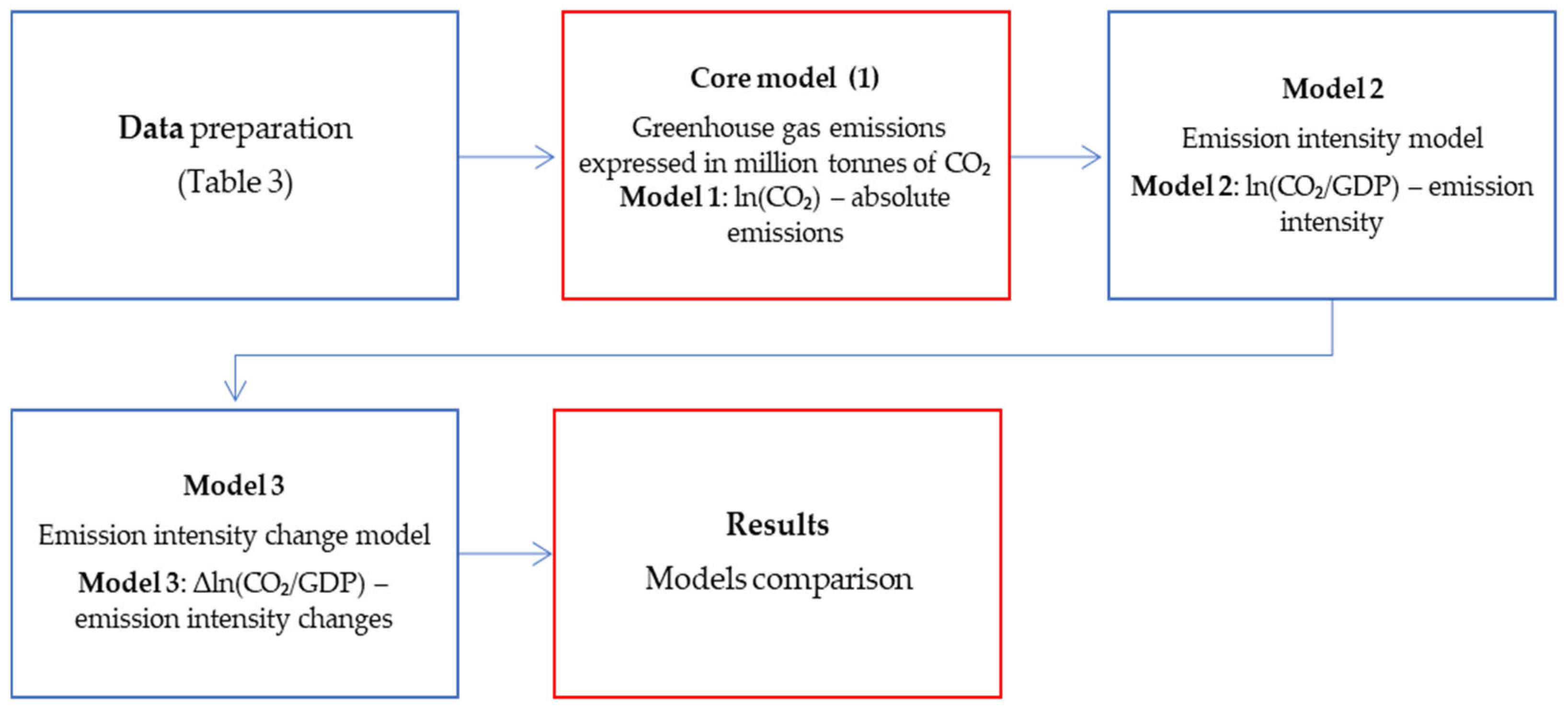
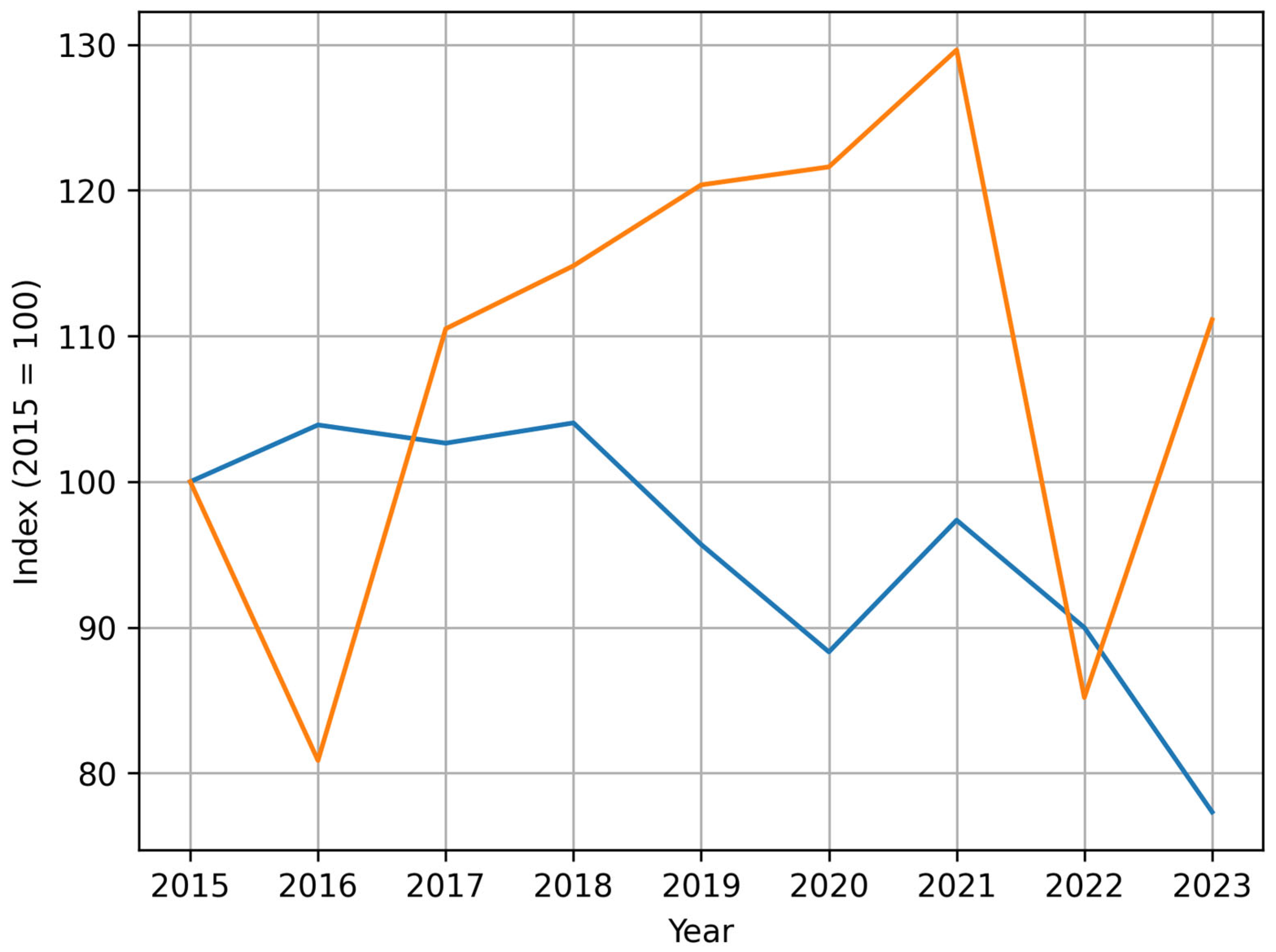
The aim of the applied methodological procedure is to empirically identify the relationships between the energy structure and CO₂ emissions in Poland, considering the level of emissions, the carbon intensity of economic growth, and the short-run dynamics of changes in emission intensity. Given the complex nature of the energy transition process, the study was designed as a multi-model analysis based on three complementary econometric specifications. Each model addresses a different research question and operates at a distinct level of informational aggregation. Model 1 addresses RQ1 and examines the impact of changes in coal consumption, natural gas consumption, and renewable energy generation on the level of absolute CO₂ emissions in Poland. Model 2 addresses RQ2 and focuses on the relationship between the energy structure and the emission intensity of economic growth, expressed as CO₂ emissions per unit of GDP. Model 3 addresses RQ3 and analyzes short-run dynamics by identifying how year-to-year changes in fossil fuel use and renewable energy production affect changes in CO₂ emission intensity. The analysis uses annual data for Poland covering the period 2015–2023 (

Table 3. Data used in analysis.

Year	RES [GWh]	CO2 Emissions [Million Tons]	Hard Coal Consumption [Million Tons]	Gas Consumption [Billion Cubic Meters]	GDP [Fixed Prices in Tens of Billions 2024]
t	RESt	${{\mathbf{CO}}_2}_{\mathit{t}}$	Coalt	Gast	GDP
2015	22,675.40	349.4	71.9	16.2	271.9
2016	22,825.36	353.9	74.7	13.1	282.7
2017	24,050.02	367.2	73.8	17.9	296.6
2018	21,579.69	368.0	74.8	18.6	310.5
2019	25,353.99	363.8	68.8	19.5	328.4
2020	28,226.56	348.1	63.5	19.7	324.4
2021	30,460.70	375.5	70.0	21.0	347.4
2022	37,671.04	344.9	64.7	13.8	354.0
2023	45,801.11	316.7	55.6	18.0	351.4

Source: Data from [104].

). Key steps of the analysis are presented in Figure 1.

The figure illustrates the co-movement between coal consumption and CO₂ emissions, with both variables following a similar trajectory, while renewable energy shows a gradual increase without a corresponding immediate decline in total emissions.

The analysis is conducted on annual data for Poland for the period 2015–2023, which further justifies the use of parsimonious and interpretable model specifications given the limited number of observations. The data sources used in the analysis (Table 3) were the official office in Poland: government website: open data/gov.pl [104].

Coal consumption clearly dominates the model, with the highest and most statistically significant coefficient, whereas the effects of other variables remain comparatively limited in magnitude and significance.

The core variable in the analysis is greenhouse gas emissions, expressed in million tons of CO₂. The explanatory variables capture the key components of the energy structure: hard coal consumption (million tons), natural gas consumption (billion cubic meters), and electricity generation from renewable energy sources (GWh), including renewables together with hydropower and co-firing. In addition, real GDP at constant prices is used as a measure of the scale of the economy.

For the purposes of the second and third models, an emission intensity variable was constructed, defined as the ratio of CO₂ emissions to GDP. This variable allows for the analysis of the carbon intensity of economic growth independently of changes in the level of economic activity. All quantitative variables were transformed logarithmically, which enables the interpretation of parameters in terms of elasticities and mitigates problems of heteroskedasticity and nonlinear relationships.

To identify the relative sensitivity of greenhouse gas emissions to changes in the energy structure, log–log regression models were employed.

The baseline emission elasticity model takes the following form (Formula (1)) on the basis of [105,106,107]:

$$\mathrm{l}\mathrm{n}({\mathrm{CO}}_2{)}_{\mathrm{t}}=\mathsf{\alpha }+{\mathsf{\beta }}_1\mathrm{l}\mathrm{n}(\mathrm{Coal}{)}_{\mathrm{t}}+{\mathsf{\beta }}_2\mathrm{l}\mathrm{n}(\mathrm{Gas}{)}_{\mathrm{t}}+{\mathsf{\beta }}_3\mathrm{l}\mathrm{n}(\mathrm{RES}{)}_{\mathrm{t}}+{\mathsf{\epsilon }}_{\mathrm{t}}$$

(1)

where:

• (CO₂)_t = energy-related carbon dioxide emissions in year t, measured in million tons
• (Coal)_t = hard coal consumption in year t, measured in million tons
• (Gas)_t = natural gas consumption in year t, measured in billion cubic meters
• (RES)_t = electricity generation from renewable energy sources in year t, measured in GWh
• t = time index denoting a given year
• ln(·) = natural logarithm; values after logarithmic transformation are treated as dimensionless
• α = intercept term (constant of the regression model); it has no physical unit
• β₁, β₂, β₃ = slope coefficients interpreted as elasticities; they are dimensionless
• ε_t = random error term in year t, representing the part of emissions not explained by the included regressors; in the log specification, it is treated as dimensionless

$${\mathsf{\beta }}_{\mathrm{i}}={\displaystyle \frac{\mathsf{\partial }\mathrm{l}\mathrm{n}\left(\mathrm{C}{\mathrm{O}}_2\right)}{\mathsf{\partial }\mathrm{l}\mathrm{n}\left({\mathrm{X}}_{\mathrm{i}}\right)}}$$

(2)

where the estimated coefficients ${\mathsf{\beta }}_{\mathrm{i}}$ represent elasticities, that is on basis [105,106,107]:

• β_i = elasticity of CO₂ emissions with respect to explanatory variable X_i; it is dimensionless
• CO₂ = energy-related carbon dioxide emissions, originally measured in million tons; after logarithmic transformation it is dimensionless
• X_i = the i-th explanatory variable included in the model; in this study it may represent:

  -

  Coal, measured in million tons

  -

  Gas, measured in billion cubic meters

  -

  RES, measured in GWh

• ∂ = partial derivative operator, indicating the marginal effect of a change in one variable while the other variables are held constant; it has no unit.

• which can be interpreted as the percentage change in CO₂ emissions resulting from a 1% change in the respective explanatory variable ${\mathrm{X}}_{\mathrm{i}}$. Such a specification is widely used in energy and environmental economics due to the nonlinear and scale-dependent nature of relationships between energy production, fuel consumption, and emissions.

After the inclusion of the interaction term between renewable energy production and coal consumption, the interpretation of the estimated coefficients fundamentally changes. In a standard log–log specification without interactions, the parameters β₁ and β₂ can be interpreted as unconditional elasticities. However, once the interaction term ln(RES) × ln(Coal) is introduced, β₁ and β₂ no longer represent standalone elasticities. Instead, the marginal impact of each variable on CO₂ emissions becomes conditional on the level of the interacting variable.

Ordinary Least Squares (OLS) is employed in this study as a theoretically grounded and methodologically appropriate estimation framework for identifying structural relationships between energy consumption variables and CO₂ emissions under conditions of limited data availability [108,109]. The choice of OLS is not motivated by convenience, but by its well-established role in environmental and energy economics as a baseline estimator for elasticity-based models, particularly when the objective is interpretative analysis rather than forecasting or causal identification.

Ordinary Least Squares (OLS) is employed as the estimation method [110]:

$$\widehat{\mathsf{\beta }}=({\mathrm{X}}^{\prime }\mathrm{X}{)}^{-1}{\mathrm{X}}^{\prime }\mathrm{Y}$$

(3)

where:

• $\widehat{\mathsf{\beta }}$ = vector of estimated regression coefficients; it is dimensionless in the log–log specification
• X = matrix of explanatory variables, including a column of ones for the intercept and the observations for the regressors; the matrix contains variables in logarithmic form and is therefore treated as dimensionless
• X′ = transpose of matrix X
• (X′X)⁻¹ = inverse of the cross-product matrix of regressors
• y = vector of the dependent variable, here ln(CO₂,_t); it is dimensionless after logarithmic transformation

From a theoretical perspective, log–log OLS specifications provide direct estimates of elasticities, which are the dominant analytical metric in empirical studies of energy demand, fuel substitution, and emission responsiveness [111,112,113,114,115]. OLS—augmented with heteroskedasticity and autocorrelation consistent (HAC) standard errors—is widely regarded as a defensible and informative estimation strategy when inferential claims are explicitly constrained [111,112,113,114,115], where the covariance matrix is estimated as [110]:

$$\widehat{\mathrm{Var}}(\widehat{\mathsf{\beta }})=({\mathrm{X}}^{\prime }\mathrm{X}{)}^{-1}\left({\sum }_{\mathrm{t}=1}^{\mathrm{T}}{\sum }_{\mathrm{s}=1}^{\mathrm{T}}{\mathrm{w}}_{\mid \mathrm{t}-\mathrm{s}\mid }{\widehat{\mathrm{u}}}_{\mathrm{t}}{\widehat{\mathrm{u}}}_{\mathrm{s}}{\mathrm{X}}_{\mathrm{t}}{\mathrm{X}}_{\mathrm{s}}^{\prime }\right)({\mathrm{X}}^{\prime }\mathrm{X}{)}^{-1}$$

(4)

where:

• $\widehat{\mathrm{V}\mathrm{a}\mathrm{r}}$($\widehat{\mathsf{\beta }}$) = estimated covariance matrix of the OLS coefficient vector; it is used to compute robust standard errors
• $\widehat{\mathsf{\beta }}$ = vector of estimated regression coefficients
• X = matrix of explanatory variables
• X_t = vector of explanatory variables for observation t; it is dimensionless in the log specification
• X_s′ = transpose of X_s
• û_t = OLS residual for observation t, that is, the estimated error term; in the log model it is dimensionless
• T = total number of observations; it has no unit
• l = lag index used in the autocovariance correction; it has no unit
• q = maximum lag length used in the HAC estimator; it has no unit
• w₁ = kernel weight assigned to lag l; it is dimensionless. In the Newey–West procedure it is defined as:

w₁ = 1 − l/(q + 1)

• (X′X)⁻¹ = inverse of the regressors’ cross-product matrix

The use of Newey–West HAC standard errors addresses the two most likely violations of classical OLS assumptions in macro–energy time series: heteroskedasticity and serial correlation of unknown form [82,83].

While Generalized Method of Moments (GMM) and related estimators are often used to address endogeneity and dynamic dependence, they are not well suited to the empirical setting of this study. GMM relies on the availability of valid and sufficiently strong instruments, which is difficult to ensure in a single-country time series with only nine annual observations. Weak or overfitted instruments in such small samples can lead to biased estimates and unreliable inference, often worse than those obtained from OLS [116,117].

To ensure the econometric validity of the estimated models, further diagnostic tests were carried out to test for multicollinearity and stationarity of the variables. The test for multicollinearity used variance inflation factors (VIFs) for each regressor in both level and different models. VIFs measure help to identify high standard errors due to strong linear relationships between the regressors, especially in the presence of a common trend. The diagnostic tests were performed for interpretational purposes rather than as exclusion criteria, as it is likely to capture relevant structural relationships in the energy transition process. Variance inflation factor [110],

$$\mathrm{V}\mathrm{I}{\mathrm{F}}_{\mathrm{j}}={\displaystyle \frac{1}{1-{\mathrm{R}}_{\mathrm{j}}^2}}$$

(5)

where

• VIF_j = variance inflation factor for the j-th explanatory variable; it is dimensionless
• R_j² = coefficient of determination obtained from the auxiliary regression in which the j-th regressor is regressed on all the other explanatory variables; it is dimensionless and ranges from 0 to 1
• j = index of the explanatory variable under consideration; it has no unit

In addition, the time-series properties of the data were evaluated using Augmented Dickey–Fuller (ADF) unit root tests applied to log-transformed variables and their first differences. The results indicate that the main variables in levels are non-stationary, while the first difference of emission intensity is stationary. These findings justify the use of alternative specifications based on normalization (CO₂/PKB) and log-differencing and support the interpretation of the dynamic model as the most appropriate framework for short-run analysis, while level-based models are treated as exploratory representations of long-run structural relationships.

The Augmented Dickey–Fuller (ADF) test is based on the regression [118]:

$$\Delta {\mathrm{y}}_{\mathrm{t}}=\mathsf{\alpha }+\mathsf{\delta }{\mathrm{y}}_{\mathrm{t}-1}+{\sum }_{\mathrm{i}=1}^{\mathrm{p}}{\mathsf{\varphi }}_{\mathrm{i}}\Delta {\mathrm{y}}_{\mathrm{t}-\mathrm{i}}+{\mathsf{\epsilon }}_{\mathrm{t}}$$

(6)

where:

• Δy_t = y_t − ${\mathrm{y}}_{\mathrm{t}-1}$ = first difference of the analyzed variable; after logarithmic transformation it is dimensionless
• y_t = analyzed time-series variable at time t; in this study it may represent ln(CO₂), ln(Coal), ln(Gas), ln(RES), or ln(INT_CO₂); all such logged variables are dimensionless
• ${\mathrm{y}}_{\mathrm{t}-1}$ = one-period lag of the analyzed variable
• α = intercept term; it is dimensionless
• δ = coefficient testing the presence of a unit root; it is dimensionless
• p = number of lagged first-difference terms included in the regression; it has no unit
• ϕ_i = coefficient on the i-th lagged first difference; it is dimensionless
• $\Delta {\mathrm{y}}_{\mathrm{t}-\mathrm{i}}$ = lagged first difference of the variable; it is dimensionless
• ε_t = random error term; it is dimensionless

In our analysis, emissions of greenhouse gases are emissions of CO₂ arising from energy consumption, excluding total economy-wide emissions from sources such as agriculture, industry, and land use changes. This matches the analytical content of the paper, which discusses the role of coal and gas consumption and the production of electricity through renewable energy sources.

CO₂ emissions are expressed in million tons and refer to emissions arising from the combustion of fossil fuels to meet energy-related needs within Poland. These emissions are derived from official national energy and emissions data and represent energy-related CO₂ emissions as defined by international energy and climate change accounting frameworks [104].

The energy system considered in this analysis is that corresponding to energy-related CO₂ emissions, considered to be the main contributor to the greenhouse effect in energy systems depending on fossil fuels. This avoids any conceptual difficulties between sectoral and economy-wide emissions and allows direct interpretation of results in terms of their implications for energy-related CO₂ emissions.

Specifically, the marginal effect of renewable energy on emissions is given by on the basis of [105,106,107]:

∂ln(CO₂)/∂ln(RES) = β₁ + β₃·ln(Coal)

(7)

where:

• ${\displaystyle \frac{\mathsf{\partial }\mathrm{l}\mathrm{n}\left(\mathrm{C}{\mathrm{O}}_2\right)}{\mathsf{\partial }\mathrm{l}\mathrm{n}\left(\mathrm{R}\mathrm{E}\mathrm{S}\right)}}$ = conditional elasticity of CO₂ emissions with respect to renewable electricity generation; it is dimensionless;
• ${\mathsf{\beta }}_1$ = coefficient associated with $\mathrm{l}\mathrm{n}\left(\mathrm{R}\mathrm{E}\mathrm{S}\right)$ in the interaction model; it is dimensionless;
• ${\mathsf{\beta }}_3$ = coefficient associated with the interaction term $\mathrm{l}\mathrm{n}\left(\mathrm{R}\mathrm{E}\mathrm{S}\right)\times \mathrm{l}\mathrm{n}\left(\mathrm{C}\mathrm{o}\mathrm{a}\mathrm{l}\right)$; it is dimensionless;
• $\mathrm{l}\mathrm{n}\left(\mathrm{C}\mathrm{o}\mathrm{a}\mathrm{l}\right)$ = natural logarithm of hard coal consumption; the original variable is measured in million tons, while the logged value is dimensionless;

• while the marginal effect of coal consumption depends on the level of renewable energy on the basis of [105,106,107]:

∂ln(CO₂)/∂ln(Coal) = β₂ + β₃·ln(RES)

(8)

where:

• ${\displaystyle \frac{\mathsf{\partial }\mathrm{l}\mathrm{n}\left(\mathrm{C}{\mathrm{O}}_2\right)}{\mathsf{\partial }\mathrm{l}\mathrm{n}\left(\mathrm{C}\mathrm{o}\mathrm{a}\mathrm{l}\right)}}$ = conditional elasticity of CO₂ emissions with respect to coal consumption; it is dimensionless;
• ${\mathsf{\beta }}_2$ = coefficient associated with $\mathrm{l}\mathrm{n}\left(\mathrm{C}\mathrm{o}\mathrm{a}\mathrm{l}\right)$ in the interaction model; it is dimensionless;
• ${\mathsf{\beta }}_3$ = coefficient associated with the interaction term $\mathrm{l}\mathrm{n}\left(\mathrm{R}\mathrm{E}\mathrm{S}\right)\times \mathrm{l}\mathrm{n}\left(\mathrm{C}\mathrm{o}\mathrm{a}\mathrm{l}\right)$; it is dimensionless;
• $\mathrm{l}\mathrm{n}\left(\mathrm{R}\mathrm{E}\mathrm{S}\right)$ = natural logarithm of renewable electricity generation; the original variable is measured in GWh, while the logged value is dimensionless.

Consequently, the coefficients reported in the paper should be interpreted as technical parameters of the interaction model rather than as direct economic elasticities. The substantive interpretation of the interaction model is therefore based on conditional marginal effects rather than on the raw coefficients themselves.

To directly address the potential influence of common deterministic trends identified in the diagnostic analysis, an additional robustness specification of the baseline model was estimated with an explicit linear time trend. This approach allows the separation of structural relationships between energy variables and emissions from general time-driven dynamics that may otherwise generate spurious correlations in level-based regressions. The inclusion of a time trend follows standard practice in short macro–energy time series where key variables exhibit strong co-movement over time.

The augmented model is specified on the basis of [105,106,107]:

$$\mathrm{l}\mathrm{n}\left({\mathrm{CO}}_{2_{\mathrm{t}}}\right)=\mathsf{\alpha }+{\mathsf{\beta }}_1\mathrm{l}\mathrm{n}\left({\mathrm{Coal}}_{\mathrm{t}}\right)+{\mathsf{\beta }}_2\mathrm{l}\mathrm{n}\left({\mathrm{Gas}}_{\mathrm{t}}\right)+{\mathsf{\beta }}_3\mathrm{l}\mathrm{n}\left({\mathrm{RES}}_{\mathrm{t}}\right)+{\mathsf{\beta }}_4\mathrm{t}+{\mathsf{\epsilon }}_{\mathrm{t}}$$

(9)

where:

• ${\mathrm{CO}}_{2_{\mathrm{t}}}$ = total carbon dioxide emissions in year $\mathrm{t}$, measured in million tons;
• $\mathrm{C}\mathrm{o}\mathrm{a}{\mathrm{l}}_{\mathrm{t}}$ = coal consumption in year $\mathrm{t}$, measured in million tons;
• $\mathrm{G}\mathrm{a}{\mathrm{s}}_{\mathrm{t}}$ = natural gas consumption in year $\mathrm{t}$, measured in billion cubic meters;
• $\mathrm{R}\mathrm{E}{\mathrm{S}}_{\mathrm{t}}$ = electricity generation from renewable energy sources in year $\mathrm{t}$, measured in GWh;
• $\mathrm{t}$ = deterministic time trend, representing calendar time (year index, e.g., 1, 2, …, T);
• $\mathrm{l}\mathrm{n}(\cdot )$ = natural logarithm; all logged variables are dimensionless.
• $\mathsf{\alpha }$ = intercept term; dimensionless;
• ${\mathsf{\beta }}_1,{\mathsf{\beta }}_2,{\mathsf{\beta }}_3$ = elasticity coefficients; dimensionless.
• ${\mathsf{\beta }}_4$ = coefficient of the time trend; it represents the average systematic change in log CO₂ emissions per unit of time (year);
• ${\mathsf{\epsilon }}_{\mathrm{t}}$ = random error term; dimensionless.

This specification serves as a direct test of whether the positive renewable energy coefficient obtained in the baseline model remains robust once common trends are explicitly controlled for, thereby providing an essential robustness check for the interpretation of level-based results.

To disentangle the impact of energy-related changes from the scale effect of the economy, an alternative specification based on emission intensity was employed. Emission intensity is defined as the ratio of CO₂ emissions to real GDP (Formula (10)) on the basis of [119,120,121]:

$${\mathrm{INT}\text{\_}\mathrm{CO}}_{2_{\mathrm{t}}}={\displaystyle \frac{{\mathrm{CO}}_{2_{\mathrm{t}}}}{\mathrm{G}\mathrm{D}{\mathrm{P}}_{\mathrm{t}}}}$$

(10)

where:

• ${{\text{INT\_CO}}_2}_{\mathrm{t}}$ = carbon emission intensity in year $\mathrm{t}$;
• ${\mathrm{CO}}_{2_{\mathrm{t}}}$ = total CO₂ emissions in year $\mathrm{t}$, measured in million tons;
• $\mathrm{G}\mathrm{D}{\mathrm{P}}_{\mathrm{t}}$ = gross domestic product in year $\mathrm{t}$, measured in constant prices (e.g., billion EUR or PLN);
• $\mathrm{t}$ = time index (year).

The emission intensity model makes it possible to assess whether changes in the energy structure led to genuine decarbonization of the economy, understood as a decline in emissions per unit of GDP. This perspective is particularly relevant in the context of climate policy, as it allows a distinction to be made between emission-intensive growth and low-emission growth.

The third model focuses on short-run dynamics and uses first differences of logarithms, which makes it possible to analyze annual changes in emission intensity and to reduce the risk of non-stationarity in the time series (Formula (11)) on the basis of [122,123,124]:

Δln(INT_CO₂_t) = α + β₁ Δln(Coal_t) + β₂ Δln(Gas_t) + β₃ Δln(RES_t) + β₄ Δln(RES_{t − 1}) + ε_t

(11)

where:

• $\Delta$ = first-difference operator, defined as $\Delta {\mathrm{x}}_{\mathrm{t}}={\mathrm{x}}_{\mathrm{t}}-{\mathrm{x}}_{\mathrm{t}-1}$; dimensionless after logarithmic transformation
• INT_CO₂_t = emission intensity at time $\mathrm{t}$, defined as CO₂_t/GDP_t; unit: e.g., tons CO₂ per unit of GDP
• ln(INT_CO₂_t) = natural logarithm of emission intensity; dimensionless
• Coal_t = coal consumption (or coal-based energy use) at time $\mathrm{t}$; unit: e.g., PJ or TWh
• Gas_t = natural gas consumption at time $\mathrm{t}$; unit: e.g., PJ or TWh
• RES_t = renewable energy consumption or share at time $\mathrm{t}$; unit depends on definition (e.g., PJ or %)
• Δln(Coal_t), Δln(Gas_t), Δln(RES_t) = short-run growth rates of respective variables; dimensionless
• Δln(RES_{t − 1})= lagged growth rate of renewable energy; captures delayed adjustment effects
• $\mathsf{\alpha }$ = intercept term; dimensionless
• ${\mathsf{\beta }}_1,{\mathsf{\beta }}_2,{\mathsf{\beta }}_3,{\mathsf{\beta }}_4$ = short-run elasticities of emission intensity with respect to changes in energy structure; dimensionless
• ε_t = error term capturing unobserved factors; assumed to be mean zero

This specification captures short-term adjustment mechanisms linking changes in the energy mix to year-to-year fluctuations in the carbon intensity of the economy.

The moderation was implemented by augmenting the baseline log–log emissions model with an interaction term between renewable electricity production and coal consumption. Specifically, all variables were expressed in natural logarithms, and the interaction term was constructed as the product of ln(RES) and ln(Coal). The estimated specification takes the following form on the basis of [125,126]:

ln(CO₂_t) = α + β₁ ln(Coal_t) + β₂ ln(Gas_t) + β₃ ln(RES_t) + β₄ [ln(Coal_t) × ln(RES_t)] + ε_t

(12)

where:

• CO₂_t = total CO₂ emissions at time $\mathrm{t}$; unit: e.g., million tons
• ln(CO₂_t) = natural logarithm of emissions; dimensionless
• Coal_t, Gas_t, RES_t = as defined above
• ln(Coal_t) × ln(RES_t) = interaction term capturing the moderation effect of renewable energy on coal-related emissions
• α = intercept term; dimensionless
• ${\mathsf{\beta }}_1$ = elasticity of emissions with respect to coal use, conditional on $\mathrm{RES}$
• ${\mathsf{\beta }}_2$ = elasticity with respect to gas use
• ${\mathsf{\beta }}_3$ = elasticity with respect to renewable energy
• ${\mathsf{\beta }}_4$ = interaction coefficient measuring how the effect of coal depends on the level of renewable energy
• ε_t = stochastic error term

• where the coefficient ${\mathsf{\beta }}_3$ captures the moderating effect of coal intensity on the relationship between renewable energy and emissions. In this framework, the marginal effect of renewable energy on CO₂ emissions is conditional on the level of coal consumption, and vice versa, allowing for non-additive and context-dependent association.

All models were estimated using ordinary least squares (OLS) with heteroskedasticity and autocorrelation consistent (HAC) standard errors to ensure robust inference given the short time series and potential serial correlation. Due to the strong trending behavior of energy variables and the limited number of observations, the moderation analysis is interpreted as an exploratory structural diagnostic rather than a causal test. Its purpose is to reveal whether interaction effects help explain why renewable energy expansion may not translate into immediate emission reductions in coal-intensive systems, thereby complementing the baseline, intensity-based, and dynamic model specifications.

Possible parameter uncertainties differ across the equations used in the study. In the baseline log–log model, the main uncertainty concerns the estimated elasticities of coal, gas, and renewable energy, which may partly reflect common trending behavior and the small number of observations rather than purely independent structural effects. In the elasticity definition itself, uncertainty is interpretive rather than algebraic, since the empirical meaning of elasticity depends on the adequacy of the regression specification. In the OLS estimator, uncertainty arises from sampling variability, possible omitted variables, and the limited time-series length, which constrain causal interpretation. In the HAC covariance estimator, uncertainty is mainly related to the choice of lag length and affects statistical inference through robust standard errors. In the VIF diagnostic, uncertainty concerns the degree to which multicollinearity inflates coefficient variances and weakens variable-specific interpretation. In the ADF test equation, uncertainty results from the low power of unit root tests in short samples, which may affect the classification of variables as stationary or non-stationary. In the interaction-based marginal effects, uncertainty is amplified because the estimated effect of one variable depends on the level of another, making the coefficients more sensitive to sample limitations and collinearity. In the trend-augmented model, uncertainty concerns whether the linear trend adequately captures the common temporal dynamics of the series. In the emission-intensity equation, uncertainty is linked to the construction of a ratio variable, since changes may reflect either decarbonization or changes in economic scale. In the first-difference dynamic model, uncertainty is associated with short-run volatility and the loss of long-run information. Finally, in the moderation model, the interaction coefficient is subject to relatively high uncertainty because interaction terms are more difficult to estimate precisely in a short sample. Taken together, these uncertainties do not undermine the validity of the study, but they require cautious interpretation of the results, especially in the level-based specifications.

The main source of uncertainties related to parameter estimates of the baseline log-log model of absolute CO₂ emissions is associated with the elasticity estimates of coal, gas, and renewable energy. Given that the degree of co-trending of energy consumption with economic activity was quite high during the 2015–2023 period, this may mean that the estimated coefficients of coal contain some partial information on common time trends. This means that the elasticity estimate of coal can be considered a conservative one, and thus its value can be interpreted as an upper bound estimate of the true elasticity value, while for gas and renewables this probability is higher.

Besides measurement errors in the explanatory variables, parameter uncertainty in the emission intensity equation (CO₂/GDP) also depends on the structure of the ratio-dependent variable, which introduces additional uncertainty into the analysis. Because GDP is included in the denominator, any uncertainty in its measurement will be passed to the dependent variable CO₂/GDP and affect the estimations. Thus, there is some scaling uncertainty in the model, so the negative elasticity of renewable energy might partly be explained by the economy’s performance and scale effects rather than pure technological ones. As a consequence, the estimated elasticity of renewable energy in the emission intensity model should be understood as the efficiency-scale elasticity rather than a technological parameter.

Parameter uncertainty is much higher in the first-difference equation used to analyze short-run changes in emission intensity because of the transformation of variables. First-differencing loses all long-run information in the equation and focuses solely on year-to-year changes, measurement errors, and short-run disturbances. Therefore, estimates are more sensitive to observations, so coefficients lose their significance and stability, which makes the analysis of structural relations problematic. In turn, the lack of significance does not imply that the relationship between two variables is weak in reality.

In the case of the model based on HAC correction, it should be noted that the uncertainty appears in relation to the robust standard error estimation and not in relation to the coefficient values. Moreover, the bandwidth and kernel choice affect the calculation of the variance-covariance matrix that, in its turn, defines the level of statistical significance of the coefficients. Therefore, it is necessary to focus on those parameters that possess marginal statistical significance, which depends on the specific correction applied to robust standard errors. In the process of checking for the presence of multicollinearity by applying the VIF criterion, parameter uncertainty appears through higher standard errors and poor interpretation of the coefficients. The negative dependence between coal usage and renewable energy production implies that the changes occur in the structure of energy markets simultaneously, and not individually, which affects the dynamics of emissions. In other words, the parameter estimates are less reliable, despite the high fitness of the whole model.

As we can see in stationarity testing (equations based on the ADF-test), there is parameter uncertainty when deciding whether a variable is stationary or not. With a small number of observations, the power of the ADF-test decreases, and thus increases the chance of error concerning the presence of unit roots. Parameter uncertainty influences model specification because in the case of potentially non-stationary variables, it could lead to spurious regression. Estimated relationships must be interpreted as reflecting a structural relationship, depending on trends. Concerning the interaction model where renewable energy and coal consumption are interacting, there is an additional concern about parameter uncertainty, as far as the interaction term is concerned. The reason why this issue is especially relevant here is that the interaction term reflects second-order relationships and hence is more likely to be influenced by data and model specifications. Small changes in the sample or the addition of a control variable may significantly influence the interaction estimation. Hence, one might consider the impact of renewable energy as structural in a world of coal dependence.

Uncertainty in parameters influences different models in different ways: in level models, it influences elasticity measurement; in intensity models, it causes scaling problems; in difference models, it increases volatility; in HAC estimates, it influences inference; in the presence of multicollinearity, it decreases interpretability; in stationarity testing, it creates issues with identification; and in higher-order interaction models, it causes instability. Consequently, the conclusions drawn from these results can be treated as robust directionally, yet approximate when it comes to magnitudes.

In

Table A1. Transformed variables used in estimation (2015–2023).

Year	ln(CO2)	ln(Coal)	ln(Gas)	ln(RES)	INT_CO2	ln(INT_CO2)	Trend
2015	5.855	4.276	2.785	10.030	1.285	0.250	0
2016	5.869	4.314	2.572	10.036	1.252	0.225	1
2017	5.906	4.302	2.886	10.089	1.238	0.214	2
2018	5.908	4.315	2.925	9.980	1.185	0.170	3
2019	5.897	4.231	2.970	10.140	1.108	0.103	4
2020	5.852	4.151	2.983	10.247	1.073	0.070	5
2021	5.928	4.248	3.045	10.323	1.081	0.078	6
2022	5.844	4.170	2.625	10.536	0.974	−0.026	7
2023	5.757	4.018	2.890	10.732	0.902	−0.103	8

,

Table A2. Multicollinearity diagnostics (VIF).

Variable	VIF
ln(Coal)	6.8
ln(Gas)	3.2
ln(RES)	7.5

,

Table A3. Stationarity tests (ADF).

Variable	ADF Statistic	p-Value
ln(CO2)	−1.21	0.67
ln(Coal)	−1.35	0.60
ln(Gas)	−1.48	0.54
ln(RES)	−0.92	0.78

and

Table A4. First differences (Δln—key variables).

Year	Δln(Coal)	Δln(Gas)	Δln(RES)	Δln(INT_CO2)
2016	0.009	−0.076	0.001	−0.025
2017	−0.003	0.114	0.005	−0.011
2018	0.003	0.014	−0.011	−0.044
2019	−0.019	0.015	0.016	−0.067
2020	−0.019	0.004	0.011	−0.033
2021	0.023	0.021	0.007	0.008
2022	−0.018	−0.147	0.020	−0.104
2023	−0.037	0.096	0.019	−0.077

, there are four supplementary tables that report the full set of transformed variables (including logarithmic, intensity, and differenced forms), as well as detailed diagnostic results for multicollinearity (VIF) and stationarity (ADF tests). These additions ensure full transparency of data processing and provide all numerical inputs required to replicate the econometric analysis presented in the manuscript.

4. Results

4.1. Basic Emission Elasticity Model

The estimation results in

Table 4. Basic emission elasticity model parameters.

Variable	Coefficient (β)	SE (HAC)	p-Value
Constant	1.026	0.979	0.295
ln(Coal)	0.753	0.133	<0.001
ln(Gas)	0.156	0.018	<0.001
ln(RES)	0.119	0.045	0.009

R² = 0.922. Adj. R² = 0.875. Coal β_coal = 0.753.

indicate a clearly differentiated strength of individual energy carriers associated with CO₂ emissions in elasticity terms. The strongest and at the same time statistically most stable determinant of emissions remains coal consumption, for which an elasticity of 0.753 implies that a 1% increase in the use of this fuel translates on average into an increase in emissions of approximately 0.75%. Natural gas exhibits a much weaker, yet still positive and statistically significant effect, which confirms its role as a fuel less emission-intensive than coal but not fully consistent with a decarbonization pathway. Energy production from renewable sources is characterized by a positive and statistically significant elasticity, suggesting that in the analyzed period the expansion of renewables occurred in parallel with rising energy demand rather than through full substitution of fossil fuels. The lack of statistical significance of the intercept, in turn, indicates that the level of emissions is largely determined by the observed energy variables rather than by an unobserved autonomous trend not captured by the model.

The estimated elasticities confirm that coal is the key driver of emission changes, as even small percentage variations in coal use lead to disproportionately large changes in CO₂ emissions, while other factors show much lower responsiveness.

A 1% increase in coal consumption leads to a 0.75% increase in CO₂ emissions. This represents a very strong and stable elasticity. Coal remains the main structural carrier of emissions, even in the final phase of the period analyzed. Natural gas β_gas = 0.156. A 1% increase in gas consumption leads to a 0.16% increase in emissions. The effect is positive, statistically significant, and several times weaker than that of coal. This empirically confirms the role of gas as a transitional fuel rather than a climate-neutral one. Renewable energy sources (RES) β_RES = 0.119. A 1% increase in RES production leads to a 0.12% increase in CO₂ emissions.

The log-log specification also facilitates interpretation of the relationships between emissions and energy variables in terms of flexibility rather than absolute changes. This is appropriate given that energy systems evolve gradually. The results suggest a hierarchy of factors that influence CO₂ emissions in Poland between 2015 and 2023. Coal is again the main driver, with a high elasticity indicating that even relatively small proportional changes in coal usage have a large effect on emission responses. This underpins its position as the main emission carrier. Natural gas also has a smaller positive elasticity, which is consistent with its role as a bridging fuel that reduces emission intensity in comparison to coal but increases emissions overall. While renewable energy has a positive elasticity in the absolute emissions model, this should not be taken to imply a causal effect on emissions. Rather, it reflects parallel growth in renewable energy supplies, overall energy demand, and economic growth. In this context, renewable energy is acting as a complement rather than a substitute for other energy sources. This suggests that we are witnessing a transitional period where growth in renewable energy supplies is limiting emission growth.

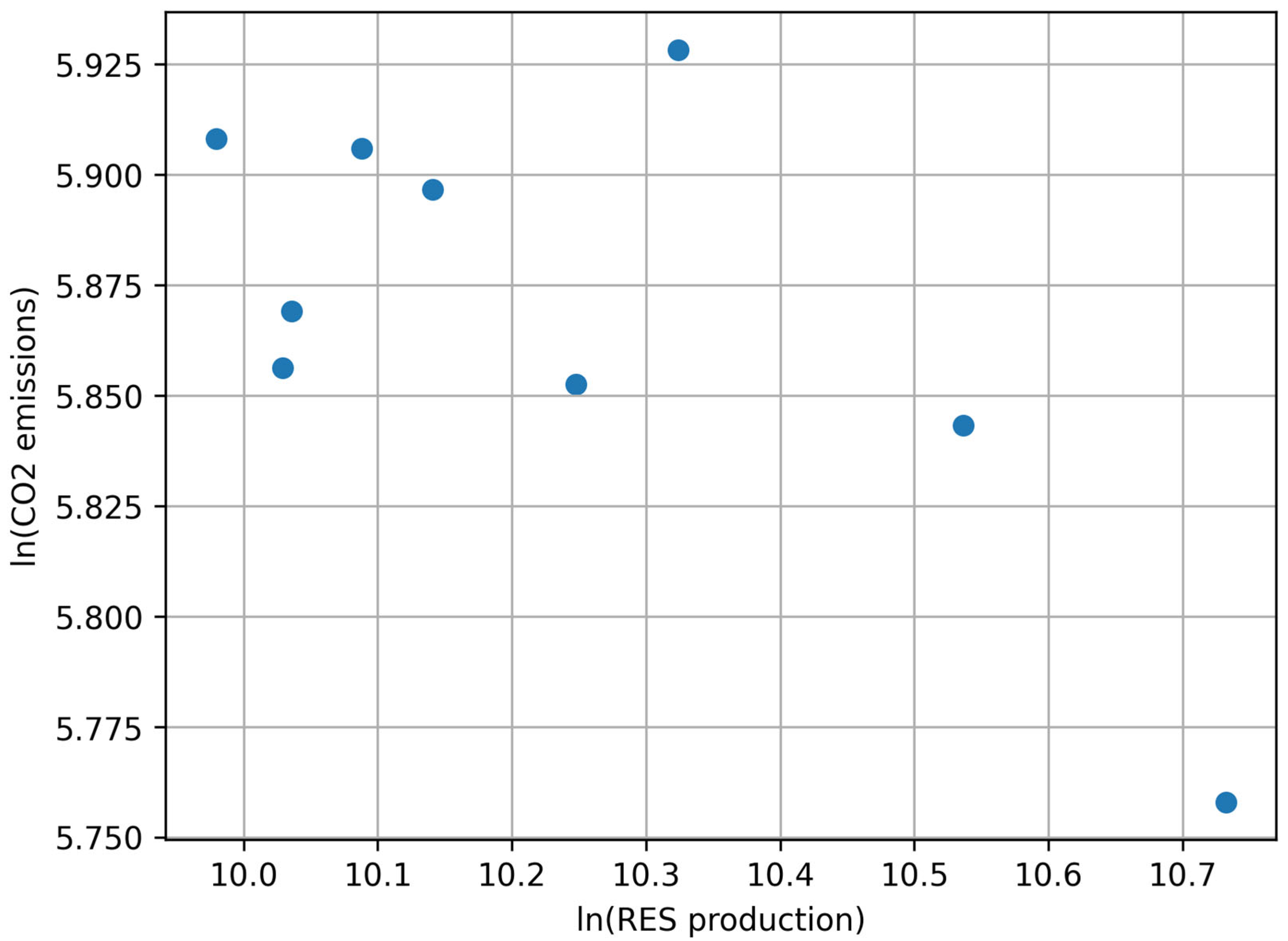
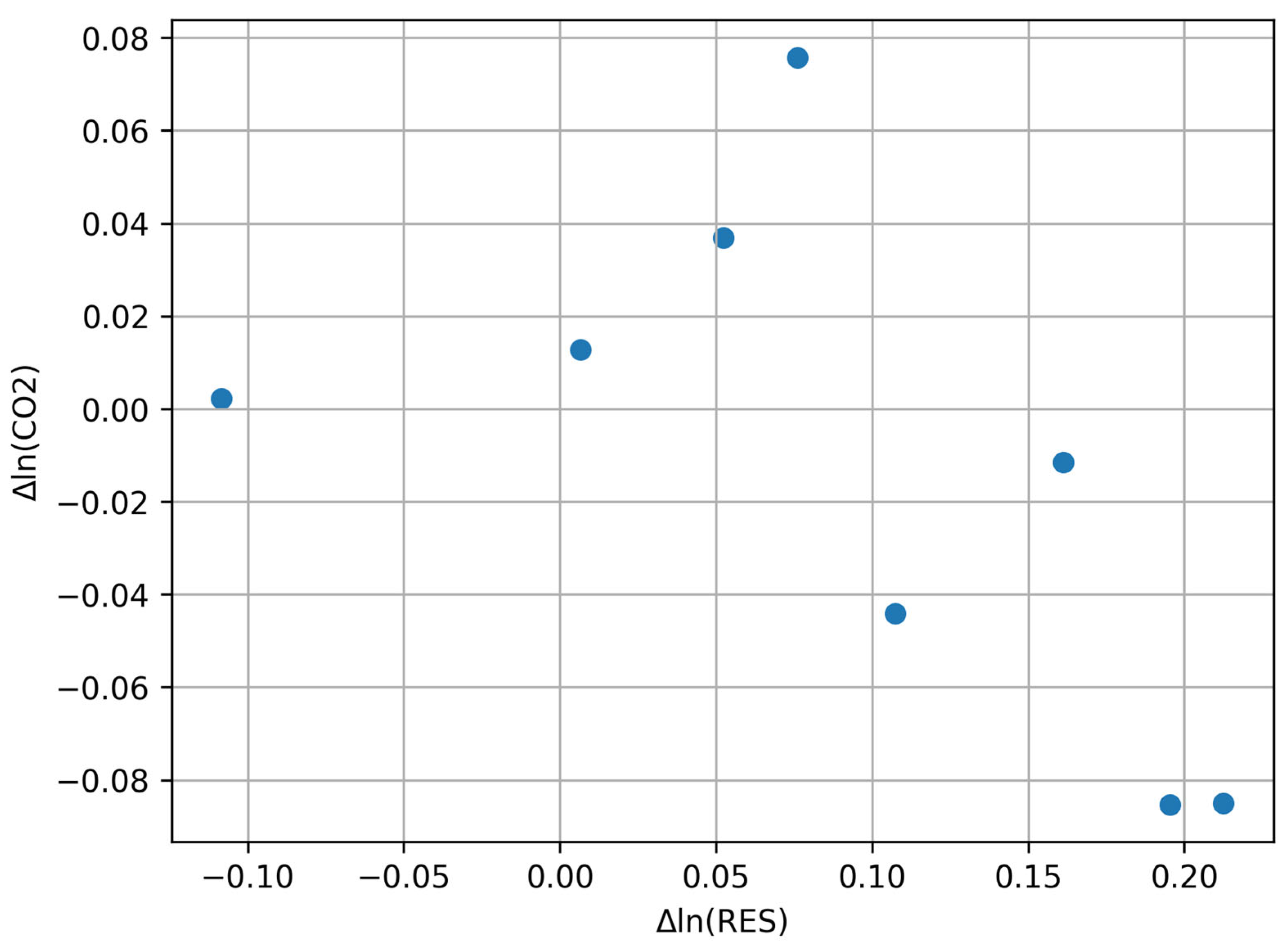
Figure 2 presents the relationship between renewable energy production and CO₂ emissions on a logarithmic scale, consistent with the elasticity-based model specification. It indicates that the observed association is influenced by common trends, which justifies the use of econometric controls in subsequent analysis.

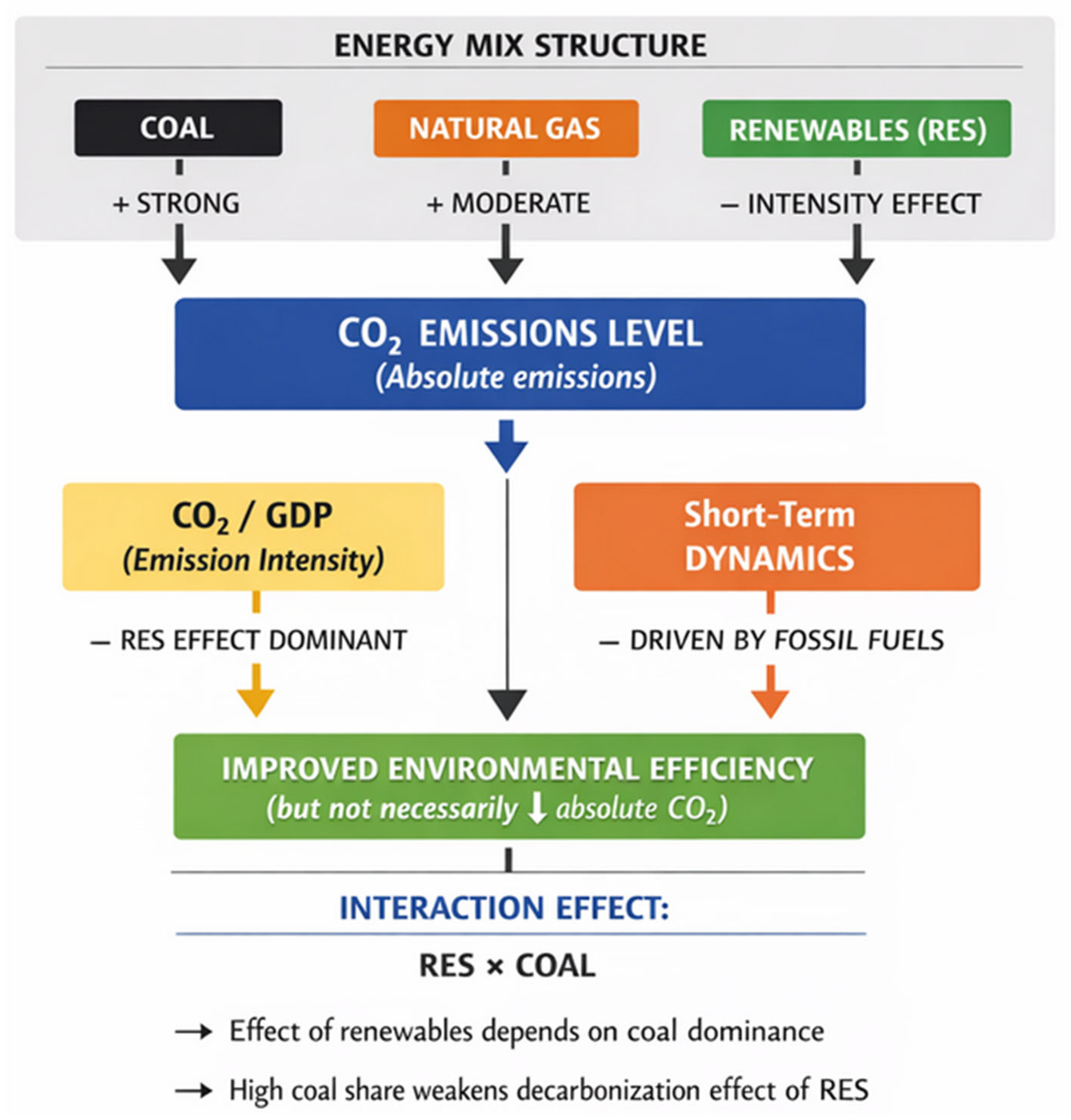
The gradual increase in renewable energy share does not fully offset the high and persistent share of coal, which explains the limited reduction in absolute emissions despite improvements in energy structure.

The picture changes when we examine the emission intensity model (CO₂/GDP). In this model, the elasticity of renewable energy is strongly negative and statistically significant, which implies that the growth in the use of this kind of energy helps to reduce the emission intensity of the economy, even if the growth in emissions is not matched by the growth in the use of this kind of energy. In this model, the coefficients on the use of coal and gas are no longer statistically significant, which implies that their impact on emission intensity is largely driven by the size of the economy rather than efficiency effects. In the dynamic models based on logarithmic differences, the changes in emission intensity in the short term are driven by fluctuations in the use of fossil fuels, whereas the impact of the use of renewable energy emerges after a lag. Only the model in which the use of renewable energy is subject to a two-year lag displays a negative relationship, which confirms the idea that the transition process displays temporal inertia.

The results suggest the following: in the first phase, the growth of renewables leads to improvement in environmental efficiency without reducing total emissions. A continuous decrease in emissions becomes possible only in the next phase, when the use of coal is significantly reduced and the role of substitution effects becomes dominant. Elasticity-based models describe this process in a clear and consistent way. From the point of view of practical policy implications, the results suggest the following: the high elasticity of coal implies that even moderate reductions in the use of this fuel lead to significant emission effects. Therefore, the use of coal is the most promising target for effective climate policy. Natural gas, although it has lower emission intensity, still adds to emissions. Therefore, it is most promising as a transitional solution rather than a long-run option. This implies that policies promoting the use of gas should remain consistent with long-run decarbonization targets.

Table A5. Correlation matrix (log-transformed variables, Pearson).

	ln(CO2)	ln(Coal)	ln(Gas)	ln(RES)	ln(Total Electricity Production)	ln(GDP)
ln(CO2)	1.000	0.830	0.289	−0.705	0.257	−0.244
ln(Coal)	0.830	1.000	−0.149	−0.906	0.116	−0.684
ln(Gas)	0.289	−0.149	1.000	0.014	−0.160	0.338
ln(RES)	−0.705	−0.906	0.014	1.000	0.300	0.806
ln(Total electricity production)	0.257	0.116	−0.160	0.300	1.000	0.412

reports Pearson correlation coefficients based on annual data for Poland (2015–2023). Bold values indicate relatively strong correlations (|r| ≥ 0.6), suggesting potential co-trending and multicollinearity concerns in level-based regressions. Variables are expressed in natural logarithms.

The direction and relative magnitude of the key coefficients remain stable across model specifications, suggesting that the dominance of coal consumption is not sensitive to model variation.

The correlation pattern of the main energy and macroeconomic variables is driven by common time trends, and this has direct consequences for the interpretability of level-based models. The strong positive correlation between renewable energy (RES) and GDP indicates that renewable energy development was closely related to economic growth and, consequently, to increasing energy demand. Thus, in this case, renewables behaved mainly as expansion drivers, not substitution drivers, supporting the potential for spurious correlation in level-based models. The strong negative correlation between RES and coal consumption reflects a long-run restructuring of the overall energy mix, where coal is gradually being substituted by renewables. However, this is a slow and long-run process, and over a short sample period, it creates high levels of multicollinearity, which may complicate coefficient estimation and interpretation in log-log models. This does not contradict the substitutive role of renewables but simply indicates that this substitution is a long-run process.

Another discrepancy in the model’s ability to diagnose is related to the negative correlation between RES and CO₂ emissions, unlike the positive elasticity of RES in the absolute emissions model. This indicates that the positive coefficient is likely driven by the coincidence of opposing trends in a single specification. These findings, in combination with the low correlation between RES and gas, indicate that there is internal heterogeneity in the energy system, thus supporting the applicability of intensity models and controlling for scale and trend effects.

Table A6. Deterministic trend analysis (log-transformed variables).

Variable	Trend Coefficient (γ)	SE (HAC)	p-Value
ln (CO2)	−0.0080	0.0069	0.246
ln (Coal consumption)	−0.0288	0.0078	<0.001
ln (RES production)	0.0843	0.0163	<0.001

reports coefficients from regressions of log-transformed variables on a linear time trend (2015 = 0). Heteroskedasticity and autocorrelation consistent (HAC) standard errors are reported. Annual data for Poland, 2015–2023.

The trend analysis indicates that there are strong deterministic patterns in all variables, which is important for understanding level-based models. RES show a strong and statistically significant trend, implying that in the period of 2015–2023, the main driver of change in renewable energy was investment and policy, and not market factors. Therefore, this is a strong trending series, implying that a statistically significant coefficient is more likely to be achieved in a level regression, even without a causal relationship to emissions. Coal consumption also has a strong and statistically significant trend, implying a long-term change in the overall energy mix. These opposing trends confirm a structural change in the transition, but they also imply a high level of multicollinearity in a short series, which may distort coefficients in models based on levels.

CO₂ emissions do not have a statistically significant trend, which has significant implications. First, despite the strong growth in RES and the decline in coal consumption, there is no evident trend in CO₂ emissions, implying that demand-side factors and economic size offset structural changes. This finding supports the view that the positive coefficient for RES in the absolute emissions model should not be taken as evidence against the decarbonization effect of renewable energy.

Table A7. Estimation results (OLS with HAC standard errors).

Variable	Coefficient (β)	SE (HAC)	p-Value	95% CI
Constant	36.998	8.413	<0.001	[20.508; 53.487]
ln (Coal)	−7.524	2.092	<0.001	[−11.624; −3.424]
ln (RES)	−3.210	0.831	<0.001	[−4.840; −1.581]
ln (Coal) × ln(RES)	0.775	0.207	<0.001	[0.370; 1.181]

reports the estimation results of the moderation model, estimated by ordinary least squares with heteroskedasticity and autocorrelation consistent (HAC) standard errors. The table shows that the effect of renewable energy on CO₂ emissions is conditional on coal intensity, as evidenced by the statistically significant interaction term, indicating non-additive and context-dependent relationships within the energy mix. R² = 0.828 Adjusted R² = 0.724. Estimation method: Ordinary Least Squares (OLS). Standard errors: Heteroskedasticity and Autocorrelation Consistent (HAC, Newey–West).

The interaction model between renewable energy (RES) and coal consumption indicates that the relationship between energy structure and CO₂ emissions is conditional rather than additive. The positive and statistically significant interaction between these variables indicates that the relationship between one variable and CO₂ emissions depends on the level of the other variable. In this case, the negative relationship between RES and CO₂ emissions is conditional upon the level of coal intensity. In essence, this indicates that the role RES can play in reducing emissions is not independent of coal intensity. In coal-dominated systems, for instance, the increase in RES will not be proportional to the reduction in emissions, since RES will be used in addition to coal rather than replacing it. It is also evident that the negative relationship between coal and CO₂ emissions is conditional upon the level of RES development.

From a methodological point of view, these results also stress the importance of not overlooking structural heterogeneity in the relationships between energy and emissions with models based on linear specifications without interaction terms. On the other hand, the very high level of statistical significance attached to the interaction term in a relatively short time series might also reflect sensitivity to co-trending and multicollinearity issues, which need to be addressed with complementary specifications, like trend-controlled or dynamic models. The results from the interaction model should thus be interpreted as structural diagnostic evidence rather than causal results.

The coefficients in Table A7 are very large and unstable, especially in comparison with the baseline model. This was to be expected due to the short sample period and the high correlation between lnRES and lnCoal. The introduction of the interaction term also leads to a redistribution of the variance in the regression equation, which might result in counter-intuitive coefficients. The coefficients are thus not to be taken at face value; rather, they are used to facilitate the computation of the estimation of the conditional effects. Substantive results are presented—these effects are computed at representative levels of coal consumption. This table shows the conditional marginal effects of renewable energy production on CO₂ emissions for three representative levels of coal consumption: the minimum, average, and maximum levels of coal consumption in the sample. The marginal effects measure the effect of the level of coal consumption on the association with renewable energy production on CO₂ emissions. The marginal effects were calculated for three representative points of the distribution of coal consumption: the minimum, the mean, and the maximum observed in the sample. This is a standard approach to the interpretation of interaction terms in log-log models.

These results show that the effect of renewable energy production on CO₂ emissions is not constant but changes depending on the coal intensity level of the energy system, becoming more positive as the level of coal use increases. The confidence intervals and HAC standard errors reported in

Table A8. Marginal effect of RES on CO₂ at representative coal levels (MERV).

Coal Level	Coal Consumption (Million Tons)	ln(Coal)	Marginal Effect of RES	SE (HAC)	95% CI
Low (minimum)	55.6	4.018	−0.094	0.036	[−0.165; −0.023]
Mean	68.64	4.225	0.066	0.057	[−0.046; 0.178]
High (maximum)	74.8	4.315	0.136	0.072	[−0.006; 0.278]

can be used to test the statistical significance of these effects.

As can be seen, the MERV analysis shows that the association with renewable energy on CO₂ emissions is not constant but varies considerably depending on the level of coal intensity used in the system. When the level of coal intensity is low, the marginal association with RES is negative and statistically significant, which means that an increase in the level of RES electricity production is associated with a decrease in emissions. However, when the level of coal intensity increases, the marginal association with RES gradually becomes weaker, eventually losing its statistical significance at the mean level and becoming positive at the highest level of coal intensity. This result again confirms that coefficients from the interaction model cannot be used as stand-alone elasticities. Rather, it suggests a conditional relationship in which the contribution of renewable energy to emission reductions is conditional upon a pre-existing moderate level of energy decarbonization, while in systems where coal is dominant, the expansion of RES seems to occur in parallel with existing fossil fuel use. This suggests a more nuanced explanation for the earlier results by level and underscores the point that the contribution of renewables in reducing emissions depends on the structural conditions of the energy system.

Table A9. Estimation results: Model 1 with explicit time trend (OLS with HAC standard errors).

Variable	β	SE (HAC)	p-Value	95% CI	Variable
Constant	2.827	0.817	0.0005	[1.225; 4.429]	Constant
ln(Coal)	0.671	0.071	<0.001	[0.532; 0.810]	ln(Coal)
ln(Gas)	0.102	0.017	<0.001	[0.070; 0.135]	ln(Gas)
ln(RES)	−0.013	0.059	0.832	[−0.129; 0.103]	ln(RES)

presents the estimation results of the baseline emissions model augmented with a linear time trend to control for common deterministic dynamics. The coefficients indicate that, once the trend is included, the previously positive elasticity of renewable energy becomes negative and statistically insignificant, while the effects of coal and gas remain positive and highly significant. The significant trend term confirms the presence of strong underlying co-trending in the data, supporting the need for trend-controlled and intensity-based specifications.

The estimation results of the extended Model 1 with explicit control for a time trend provide a direct test of the hypothesis regarding the influence of co-trending on earlier findings. After introducing a linear trend, the coefficient for ln(RES) changes sign from positive to negative and becomes entirely statistically insignificant. This indicates that the positive renewable-energy elasticity obtained in the baseline model did not reflect a genuine causal impact of renewables on emissions but was largely the result of parallel upward trends within the energy system. At the same time, the significance and stability of coal and gas remain preserved, confirming that traditional fossil fuels continue to be the primary determinants of emission levels.

The significant positive coefficient on the variable trend suggests that, during the analyzed period, there existed a general upward pressure on emissions driven by macroeconomic and demand-side factors, independent of the fuel mix structure. The inclusion of the trend effectively captures this common dynamic, allowing the model to separate structural effects from purely temporal ones. The obtained results fully confirm the validity of applying alternative specifications based on emission intensity and logarithmic differences, which mitigate problems of non-stationarity and multicollinearity. Consequently, the trend-augmented analysis constitutes key evidence that the interpretation of the level-based model must be approached with caution, and that conclusions concerning the role of renewables should rely primarily on dynamic and normalized specifications. Figure 3 shows the evolution of coal and natural gas consumption in indexed form, enabling direct comparison despite different measurement units. The results indicate a general decline in coal use alongside more variable natural gas dynamics, reflecting structural changes in the energy system. The horizontal axis represents years (2015–2023), while the vertical axis shows indexed values of fuel consumption, where 2015 = 100. The blue line represents coal consumption, while the orange line represents natural gas consumption, allowing direct comparison of their relative dynamics over time.

Although renewable energy exhibits higher relative growth rates, its lower initial base limits its impact on total emissions compared to the dominant role of coal.

4.2. Emission Intensity Model (CO₂/GDP)

Table A10. Estimation results.

Variable	Coefficient (β)	SE (HAC)	p-Value
Constant	3.390	1.651	0.040
ln(Coal)	0.192	0.190	0.312
ln(Gas)	−0.085	0.055	0.119
ln(RES)	−0.376	0.083	<0.001

R² = 0.925. Adj. R² = 0.881. β_RES = −0.376.

presents the estimation results of a log–log model in which the dependent variable is CO₂ emission intensity (CO₂/GDP), and the coefficients can be interpreted as elasticities of the economy’s emission intensity with respect to key energy carriers. The results indicate that the only factor exerting a strong and statistical association with emission intensity is renewable energy generation, for which the negative coefficient implies that an increase in renewable output leads to a systematic reduction in the carbon intensity of economic growth. Coal and natural gas consumption are not statistically significant, suggesting that in the analyzed period changes in emission intensity were not directly driven by current volumes of fossil fuel use, but rather by structural shifts in the energy mix. The statistical significance of the intercept, in turn, points to the presence of an autonomous downward trend in emission intensity that is not fully explained by the included energy variables.

A 1% increase in electricity generation from renewable energy sources leads to an approximately 0.38% reduction in emission intensity. This should be treated with caution. From a conceptual perspective, it is important to note that the negative relationship between renewable energy deployment and emission intensity is in line with expectations regarding the direction of the energy transition. Therefore, this is not a surprising or particularly new research finding. What is more significant is that this study is limited in its consideration of direct CO₂ emissions related to energy production and does not account for life-cycle-related greenhouse gas emissions related to renewable energy technologies, including those associated with raw material extraction, production, transportation, and infrastructure development. As such, this study is likely to overstate the benefits of renewable energy deployment in terms of overall environmental sustainability. Also, it is worth noting that this study does not account for supply chain emissions. As such, it is likely that this study does not fully account for the overall environmental sustainability of the transition process. This is particularly significant in relation to renewable energy technologies, where supply chain emissions may be non-negligible in relation to overall renewable energy deployment. As such, this study should be seen as a consideration of improvements in carbon intensity in relation to domestic energy production, rather than a consideration of overall environmental sustainability.

The effect of renewable energy is strong, stable, and statistically significant. The negative coefficient indicates that increasing renewable energy generation reduces the carbon intensity of the economy. Specifically, a 1% increase in renewable energy generation leads to an average reduction in emission intensity of approximately 0.38%. This confirms that renewable energy contributes to improved environmental efficiency, even if it does not immediately translate into reductions in absolute emissions. Fossil fuel variables do not exhibit statistically significant relationships with emission intensity. Coal consumption (β = 0.192), while dominant in absolute emission terms, does not significantly explain variation in emission intensity. This suggests structural saturation and limited variability within the analyzed period. Similarly, natural gas (β = −0.085) shows no statistically significant effect. Although its coefficient is negative, it is not distinguishable from zero, indicating that natural gas is neutral in terms of emission intensity—neither increasing nor effectively reducing it. This aligns with its characterization as a transitional fuel whose role depends on broader system conditions.

The model shows good stylistic fit, suggesting that emission intensity is largely driven by energy-related factors. The crucial analytical point is that the decarbonization pattern in Poland from 2015 to 2023 is dominated by changes in carbon efficiency, not changes in absolute emissions. The role of renewable energy is to be understood as a structural factor driving decarbonization by affecting long-run efficiency, not short-run changes. There is immediate relevance for policymakers. The emission intensity model changes the focus from absolute emissions to relative changes in the relationship between economic growth and pressure on the environment. The results offer evidence for policies prioritizing reductions in carbon intensity, regardless of changes in absolute emissions. This is in line with the logic of green growth and the European Green Deal, where the aim is not to limit growth but to change its carbon content.

Figure 4 illustrates the relationship between year-to-year changes in renewable energy and CO₂ emissions using first differences of logarithms. The dispersion of observations suggests a weak short-run association, supporting the regression results indicating statistical insignificance of the RES variable in the Δln model.

4.3. Emission Intensity Change Model

The

Table A11. Emission intensity changes model parameters.

Variable	β	SE (HAC)	p-Value	95% CI
Constant	−0.0346	0.00724	<0.001	[−0.0488; −0.0204]
Δln(Coal)	0.3942	0.0730	<0.001	[0.251; 0.537]
Δln(Gas)	0.0778	0.0114	<0.001	[0.0555; 0.1002]
Δln(RES)	0.0215	0.0628	0.732	[−0.102; 0.145]

R² = 0.837, Adj. R² = 0.716, Durbin–Watson ≈ 2.04.

presents the estimation results of a log–log model based on logarithmic changes (Δln), in which the dependent variable is the change in CO₂ emission intensity.

The Δln specification shows that changes in carbon intensity in Poland between 2016 and 2023 are mainly influenced by fluctuations in fossil fuel use, particularly coal, and renewables. It is a dynamic model that reveals changes in emission intensity between consecutive years by relating changes in CO₂/GDP to changes in energy input. From this specification, it is evident that coal is a major contributor to carbon intensity in Poland since its coefficient is positive and relatively high (β₁ = 0.394). This shows that a 1 percent increase in coal input will increase emission intensity by 0.39 percent. It is evident that coal is still a major contributor to carbon intensity in Poland and that a decrease in coal input will have a direct effect on environmental efficiency in the short run. Natural gas is another contributor to carbon intensity in Poland since its coefficient is positive and relatively low (β = 0.078). This shows that even though natural gas is not a major contributor to carbon intensity compared to coal, it still has a positive effect and cannot be considered a solution to carbon intensity in Poland.

Changes in renewable energy production are not statistically significant in the short run, where the coefficient is equal to 0.022 and the prob value is equal to 0.732. This indicates that, in the short term, renewable energy did not lead to a reduction in emission intensity. Therefore, renewable energy has a delayed impact on emission intensity, meaning that renewable energy has a parallel relationship with energy demand. In terms of policy, it is worth noting that, in the short term, this model indicates that decarbonization is mainly driven by a reduction in fossil fuels, especially coal. At the same time, the benefits of renewable energy appear in a long-term context. Overall, this Δln(INT_CO₂) framework is a useful policy model, particularly since it is able to identify the driving factors of yearly changes in environmental efficiency. At the same time, it is worth noting that this model did not find a short-run renewable effect, thus indicating that further research is needed, including lag structures and system constraints, in order to better understand the transition process.

4.4. Models Comparison

The comparative

Table 5. Comparison of log–log models and the emission intensity change model.

Criterion	Model 1: ln(CO2)—Absolute Emissions	Model 2: ln(CO2/GDP)—Emission Intensity	Model 3: Δln(CO2/GDP)—Emission Intensity Changes
Dependent variable	CO2 emission level	Emission intensity (CO2/GDP)	Annual change in emission intensity
Nature of analysis	Level-based, structural	Level-based, efficiency-oriented	Dynamic, short run
Interpretation of coefficients	Elasticity of absolute emissions	Elasticity of emission intensity of growth	Percentage response of changes in emission intensity
Role of coal	Very strong, positive, significant	Statistically insignificant	Strong, positive, significant
Role of gas	Positive, significant, weaker than coal	Insignificant/neutral	Positive, significant, moderate
Role of RES	Positive elasticity (no substitution)	Negative, strong, significant (decarbonization)	Insignificant in the short run
GDP scale effect	Present (implicit)	Eliminated	Eliminated
interpretive horizon	Medium- and long-term	Long-term, structural	Short-term (annual)
Main analytical insight	The system remains emission-intensive	Carbon intensity of growth is declining	Fluctuations driven by fossil fuels
Decision-making relevance	Assessment of emission pressure	Assessment of transformation effectiveness	Monitoring of current effects
Risk of misinterpretation	Confusing correlation with causality	Underestimating short-run effects	Overestimating the lack of RES effects

synthesizes three modeling approaches, showing that each captures a different dimension of the relationship between the energy structure and CO₂ emissions. The log–log model for absolute emissions focuses on the scale of emission pressure and reveals the dominant role of fossil fuels; the log–log emission intensity model shifts the emphasis toward the environmental efficiency of economic growth, highlighting the structural decarbonization effect of renewable energy sources; while the emission intensity change model identifies short-run adjustment mechanisms, in which fluctuations in carbon intensity are still driven primarily by changes in coal and natural gas consumption. Taken together, the comparison underscores the complementarity of the applied models and demonstrates that a comprehensive assessment of the energy transition requires simultaneous consideration of emission levels, emission intensity, and their dynamic evolution.

The comparison of these three applied models—log-log model of absolute emissions, log model of emission intensity, and emission intensity change model—allows for a multidimensional analysis of the energy transition process and its influence on CO₂ emissions. Although all three models analyze one and the same process, they present different perspectives on this process and allow for a reconstruction of structural and short-run aspects of carbon intensity. The absolute emissions model reveals that the energy system still heavily relies on fossil fuels, mainly coal. The positive elasticity of emissions relative to coal consumption confirms that any changes in coal consumption are reflected proportionally in emissions. However, the positive relationship between renewable energy and emissions reveals that the growth of renewable energy is a byproduct of economic growth.

The change in interpretation is evident in the emission intensity framework, where emissions are normalized by GDP. Here, renewable energy is seen to be the dominant factor, where a negative and significant coefficient confirms a decarbonization effect. This implies that, even in the absence of a consistent trend in declining emissions, economic growth is becoming increasingly less carbon intensive. The non-significance of coal and gas implies that their influence on emission intensity is more driven by overall economic scale than by fluctuations in fuel consumption. The emission intensity change model provides valuable insights into short-run adjustment mechanisms. Differences in emission intensity continue to be significantly influenced by changes in total fuel consumption, particularly coal, whereas short-run fluctuations in renewable energy consumption are non-significant.

The three models suggest the following process in the transition to the use of energy: In the first phase, the use of renewable energy affects the path of emission intensity. In the intermediate phase, the use of renewable energy improves the efficiency of economic growth in the environment. A decrease in the absolute amount of emissions occurs only in the last phase. Meanwhile, fossil fuels, despite their decreased share in the structure, continue to affect the dynamics of emissions in the short term. The integrated modeling approach demonstrates the obvious paradox: the growth of the share of renewable energy is accompanied by high emissions of CO₂. In order to assess the efficiency of the energy transition, it is necessary to consider the results of the analysis of both the level and the intensity of emissions, as well as the differences in the trends in the structure and the short term.

4.5. Tests Among Variables

Table 6. Multicollinearity diagnostics (variance inflation factors).

Model	Variable	VIF
Model 1: ln(CO2)	ln(Coal)	6.26
	ln(Gas)	1.12
	ln(RES)	6.12
Model 2: ln(CO2/PKB)	ln(Coal)	6.26
	ln(Gas)	1.12
	ln(RES)	6.12
Model 3: Δln(CO2/PKB)	Δln(Coal)	1.93
	Δln(Gas)	1.09
	Δln(RES)	1.94

reports variance inflation factors (VIFs) for the three estimated models to assess the presence of multicollinearity among regressors. The results indicate moderate multicollinearity in the level-based specifications driven by co-trending coal consumption and renewable energy production, while the differenced intensity model shows no multicollinearity concerns.

Table A12. Stationarity tests (Augmented Dickey–Fuller).

Variable	ADF Statistic	p-Value	Stationary
ln(CO2)	−0.96	0.769	No
ln(Coal consumption)	0.51	0.985	No
ln(Gas consumption)	−2.38	0.148	No
ln(RES production)	1.57	0.998	No
ln(CO2/PKB)	1.33	0.997	No
Δln(CO2/PKB)	−3.98	0.0015	Yes

reports Augmented Dickey–Fuller test statistics for log-transformed variables and for the first difference of emission intensity. The null hypothesis of a unit root cannot be rejected for variables in levels, while it is rejected for the differenced intensity measure at conventional significance levels.

The results of the multicollinearity and stationarity tests clearly confirm that the statistical properties of the data differ substantially across the analyzed model specifications, which justifies the adoption of a multi-model approach. Moderately high values of the variance inflation factor (VIF) in the level-based models indicate the presence of multicollinearity between coal consumption and renewable energy (RES) production, arising from their strong and opposing time trends. Such a configuration implies that coefficients in models estimated in levels may be sensitive to specification changes and should not be interpreted in terms of a strict causal relationship. At the same time, the absence of significant multicollinearity in the model based on first differences of logarithms confirms that shifting to a dynamic specification effectively removes the problem of co-trending and improves the stability of the estimates.

The stationarity analysis further reinforces these conclusions by showing that all key variables in logarithmic levels are non-stationary, whereas the variable capturing changes in emissions intensity is stationary. This implies that level-based models may reflect long-run structural interdependencies but are vulnerable to spurious correlation, while the differenced model satisfies the classical econometric assumptions required for short-run dynamic analysis. Consequently, the results should be interpreted jointly: level-based models provide insights into the direction and nature of the energy transition, whereas the model based on logarithmic differences constitutes the most reliable tool for assessing the contemporaneous impact of changes in energy structure on the emissions intensity of the economy.

4.6. Projections to 2050

The scenario-based projection was developed on the basis of the estimated log-log emission elasticity model, which relates CO₂ emissions to coal consumption, natural gas consumption, and renewable energy production. By applying constant annual growth rates for each of these energy forms, a projection of future emissions was developed on the basis of a multiplicative relationship in line with the estimated elasticities. This exercise is not meant to be used for a real forecast, but it is a stylized, theoretically consistent extension of the empirical model, allowing for the evaluation of long-term effects of alternative structural developments of the energy system.

Table 7. The characteristics of scenarios.

Scenario	Coal	Gas	RES
Business-as-usual	−2.0% annually	+1.5% annually	+7.0% annually
Strong transition	−6.0% annually	−1.0% annually	+10.0% annually
Demand-driven growth	−1.0% annually	+2.5% annually	+8.0% annually

provides information on the assumed annual growth rates of important energy forms that are used for developing the three projection scenarios. While Scenario A describes a moderate transition path characterized by a gradual decline in coal, a rise in natural gas, and a steady growth in renewable energy, Scenario B describes a more ambitious decarbonization path characterized by a strong decline in fossil fuels and a rapid rise in renewable energy, whereas Scenario C describes a demand-driven system where increasing demand offsets the effects of renewable energy.

Table 8. Projected CO₂ emissions (million tons).

Scenario	2023	2030	2040	2050
Business-as-usual	316.7	306.2	291.7	277.9
Strong transition	316.7	244.7	169.4	117.2
Demand-driven growth	316.7	329.0	347.4	366.8

and Figure 5 show projected emissions of CO₂ in million tons for the period between 2023 and 2050 under three alternative scenarios derived from the calculated model based on elasticity. From the results, it is clear that the pattern of emissions varies depending on the rates at which fossil fuels and renewable energy are being reduced. This indicates that the pattern of emissions is highly sensitive to energy demand and structural changes in the energy mix.

Table 9. Change in 2050 relative to 2023.

Scenario	CO2 in 2050	Change vs. 2023
Business-as-usual	277.9	−12.2%
Strong transition	117.2	−63.0%
Demand-driven growth	366.8	+15.8%

presents a summary of the long-term outcomes of all three scenarios by comparing projected CO₂ emissions in 2050 and the baseline year 2023. It is evident that only a strong transition scenario can achieve a considerable reduction in emissions, whereas a business-as-usual scenario can achieve only a minor reduction. In contrast, a demand-driven growth scenario will experience an increase in emissions, implying that renewable energy growth is not sufficient to meet the growth in energy demand.

The results obtained in the business-as-usual scenario reveal a gradual but limited decline in emissions. CO₂ emissions decrease from 316.7 million tons in 2023 to approximately 277.9 million tons in 2050. This can be interpreted as a situation where renewable energy development is quite dynamic, while fossil fuel reduction and energy demand growth are moderate. The model results reveal that under these conditions, renewable energy contributes to reducing the pressure on emissions, but the extent to which they reduce these emissions is not sufficient to lead to decarbonization. The model results also reveal that the system develops in terms of efficiency rather than structural change. The results obtained in the strong transition scenario reveal a strong and continuous decline in emissions, reaching a level of approximately 117.2 million tons in 2050. This result is mostly due to the dynamic decline in coal consumption, accompanied by moderate declines in natural gas consumption and dynamic growth in renewable energy. The results reveal that only under conditions where renewable energy development goes hand-in-hand with a decisive decline in fossil fuel consumption can we expect significant reductions in emissions. In these conditions, renewable energy acts as a substitute rather than an additional element in the energy mix.

The results obtained in the demand-driven growth scenario are the most critical in terms of providing insight into the model results. Although renewable energy development continues to grow dynamically in these conditions, emissions increase over time, reaching approximately 366.8 million tons in 2050. This result can be interpreted as a structural condition where energy demand growth exceeds the rate at which fossil fuel consumption declines. The results reveal that only through the interaction between supply-side transformation and renewable energy development can we expect to reduce emissions in absolute terms.

Based on the scenario analysis carried out in the current paper, one can conclude that under the structural features and ongoing trends of the Polish energy system, the realization of climate neutrality by 2050, which is the key goal of the European Green Deal, seems hardly possible. The use of technological substitution, especially substitution of coal-fired generation with renewables and, partially, gas-fired generation, positively impacts emission intensity. However, it cannot ensure a sufficient level of absolute emissions reduction due to structural inertia and path-dependency of the transition process identified in the empirical part of the research.

Therefore, one can suggest that decarbonization strategies focused only on technological substitution seem unlikely to work in practice. The findings show that an increase in carbon efficiency usually precedes emissions reduction. Therefore, achieving carbon neutrality requires additional efforts, and, for example, sufficiency measures might prove to be necessary. This strategy implies the reduction of demand, changes in consumption patterns, and improvement of energy efficiency. This means that in terms of policies for achieving decarbonization goals, there should be a shift from technology-driven strategies towards more holistic ones. Measures aimed at decreasing demand, for instance, in the industrial, transport, and household sectors, and altering the modes of production and consumption might serve as an essential complement to traditional strategies.

5. Discussion

5.1. Cause Analysis: Mechanisms Underlying Emission Dynamics

The results obtained from the three econometric models reveal that the determinants of CO₂ emissions in Poland are associated with its structural dependence on fossil fuels, as well as its transitional characteristics. According to the results obtained in the absolute emissions model (RQ1), the key determinant of CO₂ emissions in Poland was found to be its consumption of coal, which can be explained in the context of path dependence and technological lock-in, where past investments in the energy infrastructure based on coal have a significant influence on its present emissions [94,95,96,97,98,99,100,101,102].

On the other hand, natural gas has a lower yet still positive relationship with emissions and thus further supports the transitional role of natural gas. Although the intensity of emissions with natural gas is lower than that of coal, it is not accompanied by full decarbonization and is thus in accordance with the transitional role as mentioned in the literature [82]. One of the major results is with regard to renewable energy. Although the value is positive in the level model, this does not mean that the level of emissions actually increased but rather that the level of renewable energy and energy demand increased simultaneously. This further implies that in the period under investigation, renewable energy sources were added rather than substituted for fossil fuels. This is in accordance with the process of parallel growth, which is often observed in the early stages of energy transitions and is often accompanied by delays in structural substitution while the level of renewable energy is increasing [16,17].

The emission intensity model (RQ2) indicates that the impact of renewable energy is significant in reducing the intensity of CO₂ emissions. This suggests that the process of de-carbonization starts with the level of efficiency rather than the level of emissions. Moreover, the dynamic model (RQ3) indicates that the changes in emissions in the short run are primarily caused by the changes in fossil fuels, and the impact of renewable energy is experienced with a lag.

5.2. Comparison with Existing Literature

The results obtained in the study correlate well with the empirical research conducted in the field of energy transition and emissions. The importance of coal in the formation of absolute emissions is in accordance with the results obtained in the studies that stress the importance of fossil fuels in the formation of CO₂ emissions in the national and international arena [16,64]. Although the impact of natural gas is less significant, it is still in accordance with the studies that stress the importance of natural gas as a transitional fuel that can decrease the intensity of emissions but cannot stop them [82].

The most important point of convergence with literature relates to the differentiated impact of renewable energy on emissions. Indeed, the literature suggests that renewable energy has a positive impact on the reduction of emission intensity, without necessarily contributing to the reduction of emissions in absolute terms [16,17]. This assumption has also been confirmed by the results of the present study, in which the impact of renewable energy was found to be negative in the intensity equation, while it was positive or zero in the level equation.

The sequential nature of this energy transition process, in which the improvement of emission intensity is a prerequisite for the reduction of emissions, has also been confirmed by the results of this present study and is in accordance with the literature on the paths of decarbonization and sustainable development [18,58]. In addition, the results of this present study are also in accordance with the literature on the gradual nature of this structural change in the energy system, which is subject to various economic, institutional, and technological constraints [68,69,70].

5.3. Implications for Policy and Theory

The results have clear implications both for the formulation of the right policies in the energy sector and for the understanding of the energy transition process. First, we turn to the implications for the formulation of the right policies in the energy sector. The high elasticity of emissions in relation to the use of coal implies that the most effective way to reduce emissions is through the reduction of the use of coal. In this context, the fact that moderate reductions in the use of coal lead to significant emission reductions underlines the importance of targeted policies in this direction. With respect to the role of natural gas, it should be noted that although it leads to a lower emission intensity compared to coal, it does not provide the option for full decarbonization. Therefore, it seems that policies promoting the use of gas as a solution to the energy problem could lead to lock-in risks, which have been widely discussed in the literature [98,99,100,101,102].

At the same time, it is evident from the results that the growth in renewable energy alone is not enough for immediate reductions in absolute emissions. This has significant implications for climate policy, emphasizing the need for renewable energy growth to be accompanied by structural reductions in fossil fuel use, especially coal. From a theoretical viewpoint, it is evident that the results support an interpretation of energy transitions as a sequential and path-dependent process. In the first stage, renewable energy leads to improvements in emission efficiency (CO₂/GDP), but absolute emissions remain stable because energy demand is increasing. Only in the second stage, when fossil fuel use declines substantially, is it possible to achieve reductions in absolute emissions.

5.4. Methodological Interpretation

The results obtained in the analysis also raise a number of important methodological issues regarding the estimation of the energy-emission relationships in short time series. First, the existence of strong co-trending in the key variables—namely, renewable energy, GDP, and coal consumption—suggests that results obtained in level-based models may not be reliable in the presence of deterministic trends in the variables. The contrast between the positive renewable energy coefficient in the absolute emissions model and its negative correlation with CO₂ emissions serves to illustrate the presence of co-trending effects. This finding is also supported by the results obtained in the trend-augmented model, where the renewable energy coefficient was found to be statistically insignificant. This finding also serves to illustrate the importance of obtaining results in complementary models—namely, the emission intensity model and dynamic models based on logarithmic differences—in order to ensure the reliability of the results obtained in level-based models. The interaction model results also serve to illustrate the importance of considering the conditional nature of the relationships between the energy variables and the emissions.

Figure 6 illustrates the structure-based relationship between energy mix components such as coal, natural gas, and renewable sources of energy with their distinct impacts on carbon dioxide emissions in Poland. In this case, the use of coal is a significant determinant for absolute emissions. On the other hand, natural gas has a positive effect on emissions; however, it has a lower influence compared to coal. The impact of renewable sources is more geared towards emission intensity, and not absolute emission levels. Furthermore, the chart differentiates the structural impact from short-term dynamics that continue to be shaped by fossil fuel consumption.

5.5. Future Research Directions

The scope for further research. There are several ways in which further research could develop this analysis. One is that, by employing more data series, it may be easier to find structural relationships, thus minimizing the effects of co-trending. Another is that employing more variables, such as technological change, policy interventions, and structural change in sectors, could enhance such models. Further research could also be conducted on exploring more modeling approaches. These could include nonlinear models, share models, and system models, all of which could be useful in understanding the complexities of the energy transition process. In this context, advanced analytical tools, such as artificial intelligence, could be useful in identifying nonlinear relationships.

6. Conclusions

The results of Model 1 reveal the association between changes in the energy mix and the level of CO₂ emissions in Poland in the period 2015–2023, thereby answering RQ2. It is also observed that coal is the major contributor to the energy mix with an elasticity of 0.753. This validates the importance of coal in the energy mix of Poland. It is not only the value of the coefficients but the structural position of coal in the energy mix of Poland that makes it the dominant contributor. Natural gas has a lower elasticity but is still positive. This is in accordance with the classification of natural gas as a transitional fuel that can decrease the intensity of emissions in comparison with coal but is unable to decrease absolute emissions. In response to RQ1, the results of the regression analysis reveal the implicit presence of economic growth in the energy mix of Poland and the presence of the scale effect in the level of emissions.

The results of Model 2 reveal the association between structural changes in the energy mix and the level of CO₂ emission intensity in Poland in the period 2015–2023, thereby providing an answer to RQ2. It is observed that the expansion of renewable energy use is strongly and negatively associated with the CO₂/GDP ratio, thus validating the improvement in environmental efficiency in Poland. In contrast, coal and natural gas are not associated with the level of CO₂ emission intensity in Poland. This validates the association between the use of coal and natural gas and the level of economic activity in Poland. This is in accordance with the classification of the early and intermediate stages of energy transition in Poland, where the process takes the form of reducing emission intensity rather than reducing the absolute level of emissions.

The findings of Model 3, in relation to answering RQ3, emphasize the short-run behavior of emission intensity. Changes in CO₂ intensity over a one-year period are mainly influenced by fluctuations in fossil fuel consumption, especially coal, and then natural gas. Coal is significantly and positively correlated with changes in emission intensity, reflecting its immediate and technical effects on emission pressure. Conversely, renewable energy does not significantly influence emission intensity in the short term, implying that its effects are structural and long-term in nature.

The interaction term further provides a more refined answer to RQ3 by revealing that the relationship between renewable energy and CO₂ emissions is conditional, not additive. The statistically significant interaction term reveals that the effects of renewable energy on CO₂ emissions are conditional on coal dependence. This implies that, in a highly coal-dependent system, an increase in renewable energy does not necessarily translate proportionally into a similar proportion of emission reductions, given that new renewable capacity may be built alongside existing fossil fuel capacity.

As for the generalization potential of the proposed approach, it is limited in terms of parameter transfer but remains significant in terms of the underlying methodological structure. As the analysis has been conducted on the basis of a single-country time series (Poland, 2015–2023), the underlying coefficients may be considered unique in terms of the underlying energy mix, policy environment, and transition phase. As such, the elasticities and interaction effects derived should not be considered applicable to other countries or time periods. However, the underlying analytical structure, which relies on the use of a log-log function, first-difference dynamics, and interaction effects, may be considered applicable to alternative contexts, as long as the underlying model is re-estimated on the basis of local data.

The most promising aspect in terms of generalization potential may be considered the underlying conceptual structure of the model, including the underlying interaction effects that capture the relationship between the underlying variables in a conditional manner. This may be considered a more overarching mechanism in the context of the underlying energy transition, rather than a single-country phenomenon. However, the underlying approach may be considered limited in terms of predictive generalization potential, primarily due to the short underlying time series and the lack of out-of-sample validation. As such, the underlying approach may be considered applicable primarily in the context of explanatory analysis, which may be extended in the future by using panel data or non-linear approaches.

Possible avenues for furthering this research could include extending the framework by utilizing the tools of Artificial Intelligence in a manner that could address the issue of non-linearities, interactions, and higher-dimensional dependence that may not be captured by the conventional tools of the discipline of econometrics. For example, tools such as random forests, boosting, or even neural networks in the identification of the relationship between the structure of the energy sector and CO₂ emissions, addressing issues of multicollinearity and limitations in the underlying functional form. Furthermore, the ability of AI-based tools to conduct cross-validation and out-of-sample forecasting could further enhance the ability of the framework to forecast the underlying relationship, while still allowing for interpretation by combining the two approaches. In addition, the ability to incorporate a wider panel dataset and AI tools for feature selection could further enhance the ability of the study to generalize the underlying results.

6.1. Practical Implications

The empirical findings can be reinterpreted—somewhat cautiously—into a more operational policy architecture by aligning the estimated elasticities with specific decarbonization instruments. What emerges first is the structural weight of coal in determining absolute emission levels. This implies that short-term intervention should not rely on indirect incentives alone, but rather on enforceable reduction pathways. Binding phase-out timelines for coal-based capacity become central here, even if their implementation differs across segments of the system. Alongside this, a tightening of exposure to the EU ETS for high-emission installations would reinforce cost pressure—not uniformly, but enough to shift expectations. Public financial support for coal-linked assets should, in parallel, be progressively withdrawn—perhaps not abruptly, but in a clearly signaled sequence.

There are necessary complementary mechanisms. A redesign of capacity markets could help stabilize the system during the withdrawal phase, especially under conditions of supply uncertainty. Permitting procedures for low-emission generation—currently fragmented and often slow—would need acceleration; otherwise, investment signals remain partly ineffective. In addition, targeted financial instruments directed at coal-dependent regions may reduce the socio-economic friction of transition. Without this, resistance accumulates. Over time, these measures should be embedded within a broader structural strategy, one that extends beyond electricity generation. Coal substitution in energy-intensive industries becomes relevant here, though the pathways are heterogeneous: electrification of processes in some cases, hydrogen deployment in others, and, where substitution is technologically constrained, carbon capture solutions. Not all at once. Not evenly.

At the same time, the role of renewable energy—more nuanced than it first appears—points toward a different policy requirement. Its primary effect operates through emission intensity reduction rather than immediate cuts in absolute emissions. This suggests that general declarations about RES expansion are insufficient. Qualification is needed. Clearly defined capacity trajectories, for instance annual increments in wind and solar installations, provide a more actionable framework. Yet expansion alone does not resolve system constraints. It must be accompanied by parallel investments in grid infrastructure, storage capabilities, and mechanisms of demand-side flexibility. Otherwise, integration gaps emerge, and the decarbonization effect remains partial.

In this configuration, renewable energy acts as a necessary condition, but not a self-sufficient one. Additional clean capacity may coexist with fossil-based generation instead of replacing it, especially under conditions of rising demand. Hence, policy design should explicitly combine RES growth with constraints on fossil fuel use, ensuring actual displacement rather than mere supplementation. Within this mix, natural gas occupies an intermediate position. It contributes to system stability, yes, but its role should remain temporally bounded. Sunset conditions, clearly defined in advance, become essential to avoid long-term lock-in. Otherwise, the transition risks slowing down just as it begins to take shape.

At the same time, the translation of these policy orientations into practice encounters a set of structural constraints that shape not only feasibility, but also timing—and sometimes sequencing in a non-trivial way. Financing appears as the most immediate bottleneck. Large-scale investments in renewable generation, grid reinforcement, and storage systems require capital that is both patient and predictable. Yet this predictability depends on regulatory stability, which is rarely perfect. Even small signals of policy inconsistency can shift investment horizons. Or delay them. Long-term capital commitments, especially in infrastructure-heavy sectors, remain highly sensitive to such uncertainty.

There is also the technical layer. Grid integration, often treated as a secondary issue, becomes a binding constraint in systems with a growing share of variable renewable energy sources. Transmission capacity may lag behind generation expansion. Flexibility options—storage, demand response, interconnections—are not always sufficiently developed. As a result, part of the installed renewable capacity may remain underutilized. Curtailment increases. The system, in a sense, absorbs more than it can efficiently process. Not continuously, but often enough to matter for overall effectiveness. Social acceptance introduces another dimension, less quantifiable yet equally consequential. In regions structurally dependent on coal, the transition is not only technological but socio-economic. Employment structures, local fiscal revenues, even identity—these elements create inertia. Resistance does not always manifest openly; sometimes it appears as delay, administrative friction, political hesitation The pace of transformation therefore becomes uneven, spatially differentiated, and difficult to standardize.

Under such conditions, the sequencing of policy instruments gains strategic importance. Early-stage interventions should concentrate on enabling conditions: expansion of grid infrastructure, stabilization of regulatory frameworks, and the establishment of credible support mechanisms for regions exposed to structural change. Only then—though not strictly linearly—can accelerated deployment of renewable energy be pursued more effectively, followed by progressively tighter constraints on fossil fuel use. A staged approach, not entirely smooth but adaptive, reduces the risk of systemic imbalance. It allows the transition to unfold with fewer disruptions, increasing the probability that decarbonization objectives are met without destabilizing the broader energy system.

6.2. Limitations

This origin of data provides a certain level of institutional coherence and comparability across variables, although not without its own implicit constraints. The dataset is therefore consistent in a formal sense yet embedded in administrative reporting structures that evolve over time. Still, it remains one of the more stable empirical bases available for this type of analysis. At the same time, the temporal dimension of the dataset—relatively short, somewhat compressed—introduces methodological frictions that cannot be ignored. The number of observations is limited. This directly reduces the degrees of freedom in the estimated models, and therefore, the statistical inference becomes less robust than in longer time series settings. Parameter estimates may appear precise, but this precision is partly illusory; it depends strongly on the specific realization of the sample. Hypothesis testing, in turn, operates under constrained power conditions, which increases the risk of both Type I and Type II errors. Not always symmetrically.

References

1. Report of the World Commission on Environment and Development (1987): Our Common Future. Available online: https://sustainabledevelopment.un.org/content/documents/5987our-common-future.pdf (accessed on 14 December 2025).
2. IEA. Net Zero by 2050; IEA: Paris, France, 2021; Available online: https://www.iea.org/reports/net-zero-by-2050 (accessed on 6 March 2024).
3. European Commission. A European Green Deal: Striving to Be the First Climate-Neutral Continent. COM(2019) 640 Final. 2020. Available online: https://ec.europa.eu/newsroom/know4pol/items/664852/en (accessed on 21 December 2025).
4. EU COM. Communication from the Commission to the European Parliament, the Council, the European Economic and Social Committee and the Committee of the Regions a Roadmap for Moving to a Competitive Low Carbon Economy in 2050; European Commission (EU COM): Brussels, Belgium, 2011. [Google Scholar]
5. Devis, A. The Renewable Energy Directive III and the streamlining of environmental procedures: A paradigm shift in EU environmental policy? J. Environ. Law 2025, 37, 443–466. [Google Scholar] [CrossRef]
6. RePowerEU. Available online: https://eur-lex.europa.eu/legal-content/EN/TXT/?uri=COM:2022:230:FIN&qid=1653033742483 (accessed on 20 December 2025).
7. Directive (EU) 2023/1791 of the European Parliament and of the Council of 13 September 2023 on Energy Efficiency and Amending Regulation (EU) 2023/955 (Recast) (Text with EEA Relevance). Available online: https://eur-lex.europa.eu/legal-content/EN/TXT/?uri=OJ%3AJOL_2023_231_R_0001&qid=1695186598766 (accessed on 20 December 2025).
8. The Paris Agreement. COP21. UN Climate Change Conference (COP21) in Paris, France, on 12 December 2015. It Entered into Force on 4 November 2016. Available online: https://treaties.un.org/pages/ViewDetails.aspx?src=TREATY&mtdsg_no=XXVII-7-d&chapter=27&clang=_en (accessed on 10 January 2026).
9. Graham, E.; Fulghum, N.; Altieri, K. Global Electricity Review 2025, Ember. 8 April 2025; Available online: https://ember-energy.org/app/uploads/2025/04/Report-Global-Electricity-Review-2025.pdf (accessed on 10 January 2026).
10. Global Energy Review 2025. Coal. IEA. Available online: https://www.iea.org/reports/global-energy-review-2025/coal (accessed on 10 January 2026).
11. Pianta, M.; Lucchese, M. Rethinking the European Green Deal: An industrial policy for a just transition in Europe. Rev. Radic. Political Econ. 2020, 52, 633–641. [Google Scholar] [CrossRef]
12. Manowska, A.; Bluszcz, A.; Chomiak-Orsa, I.; Wowra, R. Towards usability: A case study of an EU country. Energies 2024, 17, 1778. [Google Scholar] [CrossRef]
13. Ellabban, O.; Abu-Rub, H.; Blaabjerg, F. Renewable energy resources: Current status, future prospects and their enabling technology. Renew. Sustain. Energy Rev. 2014, 39, 748–764. [Google Scholar] [CrossRef]
14. Gajdzik, B.; Wolniak, R.; Grebski, W.W. Structural Drivers of Poland’s Renewable Energy Transition (2010–2023): Empirical Insights from Regression and Cluster Analysis. Energies 2025, 18, 4754. [Google Scholar] [CrossRef]
15. Jaro’n, A.; Borucka, A. Analysis of Energy System Transformations in the European Union. Energies 2024, 17, 6181. [Google Scholar] [CrossRef]
16. Hanif, I.; Aziz, B.; Sharif, I.; Chaudhry, I. Carbon emissions across the spectrum of renewable and nonrenewable energy use in developing economies of Asia. Renew. Energy 2019, 143, 586–595. [Google Scholar] [CrossRef]
17. Gardiner, R.; Hájek, P. Interactions among Energy Consumption, CO2, and Economic Development in European Union Countries. Sustain. Dev. 2020, 28, 723–740. [Google Scholar] [CrossRef]
18. Sala, D.; Liashenko, O.; Pyzalski, M.; Pavlov, K.; Pavlova, O.; Durczak, K.; Chornyi, R. The Energy Footprint in the EU: How CO2 Emission Reductions Drive Sustainable Development. Energies 2025, 18, 3110. [Google Scholar] [CrossRef]
19. Gajdzik, B.; Sroka, W.; Vveinhardt, J. Energy Intensity of Steel Manufactured Utilising EAF Technology as a Function of Investments Made: The Case of the Steel Industry in Poland. Energies 2021, 14, 5152. [Google Scholar] [CrossRef]
20. Wolniak, R.; Saniuk, S.; Grabowska, S.; Gajdzik, B. Identification of Energy Efficiency Trends in the Context of the Development of Industry 4.0 Using the Polish Steel Sector as an Example. Energies 2020, 13, 2867. [Google Scholar] [CrossRef]
21. Gajdzik, B.; Nagaj, R.; Wolniak, R.; Bałaga, D.; Žuromskaite, B.; Grebski, W.W. The share of renewable energy in European industry: Analysis and extrapolation of trends in EU countries. Energies 2024, 17, 2476. [Google Scholar] [CrossRef]
22. Komarnicka, A.; Murawska, A. Comparison of Consumption and Renewable Sources of Energy in European Union Countries—Sectoral Indicators, Economic Conditions and Environmental Impacts. Energies 2021, 14, 3714. [Google Scholar] [CrossRef]
23. Androniceanu, A.; Sabie, O.M. Overview of Green Energy as a Real Strategic Option for Sustainable Development. Energies 2022, 15, 8573. [Google Scholar] [CrossRef]
24. Nagaj, R.; Gajdzik, B.; Wolniak, R.; Grebski, A. The impact of deep decarbonization policy on the level of greenhouse gas emissions in the European Union. Energies 2024, 17, 1245. [Google Scholar] [CrossRef]
25. Explanation of the Index by Eurostat. Available online: https://ec.europa.eu/eurostat/statistics-explained/index.php?title=Energy_statistics_-_an_overview (accessed on 10 January 2026).
26. Kyoto Protocol, UNFCCC. 11 December 1997. Available online: https://unfccc.int/process-and-meetings/the-kyoto-protocol (accessed on 10 January 2026).
27. EEA. Share of Energy Consumption from Renewable Sources in Europe. 6 November 2025. Available online: https://www.eea.europa.eu/en/analysis/indicators/share-of-energy-consumption-from (accessed on 29 December 2025).
28. Report IEA: Renewables 2025–Analysis–IEA. Available online: https://iea.blob.core.windows.net/assets/76ad6eac-2aa6-4c55-9a55-b8dc0dba9f9e/Renewables2025.pdf (accessed on 20 December 2025).
29. Chen, C.-C. Comparative impacts of energy sources on environmental quality: A five-decade analysis of Germany’s Energiewende. Energy Rep. 2024, 11, 3550–3561. [Google Scholar] [CrossRef]
30. Bourliaguet, B. Rethinking the energy transition: Sufficiency and the French strategy. Energy Res. Soc. Sci. 2025, 124, 104055. [Google Scholar] [CrossRef]
31. Di Nucci, M.R.; Prontera, A. The Italian energy transition in a multilevel system: Between reinforcing dynamics and institutional constraints. Z. Für Polit. 2021, 33, 181–204. [Google Scholar] [CrossRef]
32. Garha, N.S.; Mira, R.G.; González-Laxe, F. Energy Transition Narratives in Spain: A Case Study of as Pontes. Sustainability 2022, 14, 11177. [Google Scholar] [CrossRef]
33. RED III; EU. Directive (EU) 2023/2413 of the European Parliament and of the Council of 18 October 2023 Amending Directive (EU) 2018/2001, Regulation (EU) 2018/1999 and Directive 98/70/EC as Regards the Promotion of Energy from Renewable Sources, and Repealing Council Directive (EU) 2015/652. Available online: https://eur-lex.europa.eu/legal-content/EN/TXT/?trk=feed_main-feed-card_feed-article-content&uri=OJ%3AL_202302413 (accessed on 10 January 2026).
34. IEO Report: SUMMARY—„Photovoltaic Market in Poland 2025”. Intitute of Renewable Energy. Available online: https://ieo.pl/en/pv-report (accessed on 10 January 2026).
35. Gajdzik, B.; Wolniak, R.; Grebski, W.-W. Poland’s renewable energy transition (2010–2023): A fuzzy time series and multi-criteria assessment of transition quality in electricity production. Energies 2026, 19, 1248. [Google Scholar] [CrossRef]
36. Gajdzik, B.; Jaciow, M.; Wolniak, R.; Wolny, R.; Grebski, W.W. Energy Behaviors of Prosumers in Example of Polish Households. Energies 2023, 16, 3186. [Google Scholar] [CrossRef]
37. Governmental Program: Mój Prąd. Available online: https://mojprad.gov.pl/ (accessed on 10 January 2026).
38. Report Wind Energy in Poland 2025, 12th Edition. TPA Poland. Available online: https://windenergy-tpa.pl/en/ (accessed on 10 January 2026).
39. Polityka Energetyczna Polski do 2040 (PEP 2040). Document of Polish Government. Available online: https://www.gov.pl/web/ia/polityka-energetyczna-polski-do-2040-r-pep2040 (accessed on 10 January 2026).
40. Chomać-Pierzecka, E.; Kowalska, M.; Czyrka, K. The problem of transforming the energy system towards renewable energy sources as perceived by inhabitants of rural areas in South-eastern Poland. Energies 2025, 18, 5548. [Google Scholar] [CrossRef]
41. Zalewski, K.; Bórawski, P.; Żuchowski, I.; Parzonko, A.; Holden, L.; Rokicki, T. The Efficiency of Public Financial Support Investments into Dairy Farms in Poland by the European Union. Agriculture 2022, 12, 186. [Google Scholar] [CrossRef]
42. Report IRENA: Renewable Capacity Statistics 2025. International Renewable Energy Agency, Abu Dhabi. Available online: https://www.irena.org/-/media/Files/IRENA/Agency/Publication/2025/Mar/IRENA_DAT_RE_Capacity_Statistics_2025.pdf (accessed on 20 December 2025).
43. Ojczyk, J. Raport o ETS. Gdzie Jesteśmy i Dokąd Zmierzamy? KE Twierdzi, że System działa. 18 March 2026, 7:02. Business Insider. Available online: https://businessinsider.com.pl/prawo/firma/unijny-system-ets-dziala-ekspert-wyjasnia-co-to-oznacza-dla-polski/hx9375r (accessed on 30 March 2026).
44. Palusiński, B. ETS and CO2 prices: Why Does Poland Pay Some of the Highest Energy Bills in Europe? Available online: https://enerace.eu/blog/ets-co2-impact-on-energy-prices (accessed on 30 March 2026).
45. Gajdzik, B. The road of Polish steelworks towards market success—Changes after restructuring process. Metalurgija 2013, 52, 421–424. [Google Scholar]
46. Gajdzik, B.; Wolniak, R.; Grebski, W. Process of Transformation to Net Zero Steelmaking: Decarbonisation Scenarios Based on the Analysis of the Polish Steel Industry. Energies 2023, 16, 3384. [Google Scholar] [CrossRef]
47. Gajdzik, B.; Wolniak, R.; Sączewska-Piotrowska, A.; Grebski, W.W. Polish Steel Production Under Conditions of Decarbonization—Steel Volume Forecasts Using Time Series and Multiple Linear Regression. Energies 2025, 18, 1627. [Google Scholar] [CrossRef]
48. European Commission. A European Steel and Metals Action Plan. 2025. Available online: https://single-market-economy.ec.europa.eu/document/download/7807ca8b-10ce-4ee2-9c11-357afe163190_en?filename=Communication%20-%20Steel%20and%20Metals%20Action%20Plan.pdf (accessed on 21 February 2026).
49. Gajdzik, B. Digital Transformation Towards Smart Steel Manufacturing: A Framework for Steel Enterprises in Poland; Palgrave Macmillan: New York, NY, USA, 2025; ISBN 978-3-031-77755-4. [Google Scholar]
50. World Steel Association. World Steel in Figures 2024. Available online: https://worldsteel.org/wp-content/uploads/World-Steel-in-Figures-2024.pdf (accessed on 21 February 2026).
51. Wpływ Branży Cementowej na Gospodarkę Polski. August 2020. Available online: https://www.polskicement.pl/content/uploads/2025/01/Raport-Wplywu-EY-SPC-2020.pdf (accessed on 30 March 2026).
52. Sobkiewicz, M.; Krawiec, K. Przemysł Net-Zero. In Dekarbonizacja bez Utraty Konkurencyjności; Policy Paper, nr 4; Polski Instytut Ekonomiczny: Warsaw, Poland, 2025. [Google Scholar]
53. Miniszewski, M.; Pilszyk, M. Czas na Polski CCS? Szanse i Wyzwania Wychwytu i Składowania CO2 w Polskim Przemyśle. 2024. Available online: https://pie.net.pl/wp-content/uploads/2024/07/Polski-CCS-co2.pdf (accessed on 21 February 2026).
54. Przemysł Chemiczny w Polsce. Pozycja, Wyzwania, Perspektywy, Polska Izba Przemysłu Chemicznego. 2024. Available online: https://pipc.org.pl/najnowszy-raport-przemysl-chemiczny-w-polsce-pozycja-wyzwania-perspektywy-pobierz-3 (accessed on 21 February 2026).
55. Czernicka, Z. Akademia SCG: Dlaczego Polska ma Najdroższy Prąd w Europie? 12 December 2024. Available online: https://akademiaesg.pl/baza-wiedzy/dlaczego-polska-ma-najdrozszy-prad-w-europie/ (accessed on 21 February 2026).
56. Draghi, M. The Draghi Report: The Future of European Competitiveness. Part B In-Depth Analysis and Recommendations. 2024. Available online: https://commission.europa.eu/document/download/ec1409c1-d4b4-4882-8bdd-3519f86bbb92_en?filename=The%20future%20of%20European%20competitiveness_%20In-depth%20analysis%20and%20recommendations_0.pdf (accessed on 21 February 2026).
57. Mobarakeh, M.R.; Kienberger, T. Climate neutrality strategies for energy-intensive industries: An Austrian case study. Clean. Eng. Technol. 2022, 10, 100545. [Google Scholar] [CrossRef]
58. van Vuuren, D.P.; Stehfest, E.; Gernaat, D.E.H.J.; Doelman, J.C.; van den Berg, M.; Harmsen, M.; de Boer, H.S.; Bouwman, L.F.; Daioglou, V.; Edelenbosch, O.Y.; et al. Energy, land-use and greenhouse gas emissions trajectories under a green growth paradigm. Glob. Environ. Change 2017, 42, 237–250. [Google Scholar] [CrossRef]
59. Joung, T.-H.; Kang, S.-G.; Lee, J.-K. The IMO initial strategy for reducing Greenhouse Gas(GHG) emissions, and its follow-up actions towards 2050. J. Int. Marit. Saf. Environ. Aff. Shipp. 2020, 4, 1–7. [Google Scholar] [CrossRef]
60. Moreno, J.; Campagnolo, L.; Boitier, B.; Nikas, A.; Koasidis, K.; Gambhir, A.; Gonzalez-Eguino, M.; Perdana, S.; Van de Ven, D.-J.; Chiodi, A.; et al. The Impacts of Decarbonization Pathways on the Sustainable Development Goals in the European Union. Commun. Earth Environ. 2024, 5, 136. [Google Scholar] [CrossRef]
61. Taušová, M.; Mykhei, M.; Čulkova, K.; Tauš, P.; Petráš, D.; Kaňuch, P. Development of the Implementation of Renewable Sources in EU Countries in Heating and Cooling, Transport, and Electricity. Sustainability 2025, 17, 766. [Google Scholar] [CrossRef]
62. Gajdzik, B.; Wolniak, R.; Grebski, W.W. An Econometric Model of the Operation of the Steel Industry in POLAND in the Context of Process Heat and Energy Consumption. Energies 2022, 15, 7909. [Google Scholar] [CrossRef]
63. Gajdzik, B.; Jaciow, M.; Wolniak, R.; Wolny, R.; Grebski, W.W. Assessment of Energy and Heat Consumption Trends and Forecasting in the Small Consumer Sector in Poland Based on Historical Data. Resources 2023, 12, 111. [Google Scholar] [CrossRef]
64. Keles, D.; Yilmaz, H.Ü. Decarbonisation through Coal Phase-out in Germany and Europe—Impact on Emissions, Electricity Prices and Power Production. Energy Policy 2020, 141, 111472. [Google Scholar] [CrossRef]
65. Ocelík, P.; Diviák, T.; Lehotský, L.; Svobodová, K.; Hendrychová, M. Facilitating the Czech Coal Phase-Out: What Drives Inter-Organizational Collaboration? Soc. Nat. Resour. 2022, 35, 705–724. [Google Scholar] [CrossRef]
66. Lapčík, V.; Lapčík, M.; Lapčík, V., Jr. Current Aspects of Decarbonisation in the Czech Republic and Possibilities of Replacement of Coal Energy Sources by Renewable Sources of Electric Energy. J. Pol. Miner. Eng. Soc. 2022, 6, 87–96. [Google Scholar] [CrossRef]
67. International Monetary Fund. European Dept. Enhancing the Green Transition in Czech Republic. 5 November 2025. Available online: https://www.elibrary.imf.org/view/journals/002/2024/029/article-A003-en.xml (accessed on 10 January 2026).
68. Tobór-Osadnik, K.; Gajdzik, B.; Strzelec, G. Configurational Path of Decarbonisation Based on Coal Mine Methane (CMM): An Econometric Model for the Polish Mining Industry. Sustainability 2023, 15, 9980. [Google Scholar] [CrossRef]
69. Gajdzik, B.; Tobór-Osadnik, K.; Wolniak, R.; Grebski, W.W. European Climate Policy in the Context of the Problem of Methane Emissions from Coal Mines in Poland. Energies 2024, 17, 2396. [Google Scholar] [CrossRef]
70. Brauers, H.; Oei, P.Y. The Political Economy of Coal in Poland: Drivers and Barriers for a Shift Away from Fossil Fuels. Energy Policy 2020, 144, 111621. [Google Scholar] [CrossRef]
71. Pepłowska, M. Climate Neutrality in Poland: The Role of the Coal Sector in Achieving the 2050 Goal. Polityka Energ.—Energy Policy J. 2025, 28, 113–126. [Google Scholar] [CrossRef]
72. Tobór-Osadnik, K.; Korski, J.; Gajdzik, B.; Wolniak, R.; Grebski, W. Gravity Energy Storage and Its Feasibility in the Context of Sustainable Energy Management with an Example of the Possibilities of Mine Shafts in Poland. Energies 2025, 18, 3374. [Google Scholar] [CrossRef]
73. Sroka, W.; Cygler, J.; Gajdzik, B. The Transfer of Knowledge in Intra-Organizational Networks: A Case Study Analysis. Organizacija 2014, 47, 24–34. [Google Scholar] [CrossRef]
74. Zhou, C.; Richardson-Barlow, C.; Fan, L.; Cai, H.; Zhang, W.; Zhang, Z. Towards organic collaborative governance for a more sustainable environment: Evolutionary game analysis within the policy implementation of China’s net-zero emissions goals. J. Environ. Manag. 2025, 373, 123765. [Google Scholar] [CrossRef]
75. Standar, A.; Kozera, A.; Satoła, Ł. The Importance of Local Investments Co-Financed by the European Union in the Field of Renewable Energy Sources in Rural Areas of Poland. Energies 2021, 14, 450. [Google Scholar] [CrossRef]
76. Dzikuć, M.; Kuryło, P.; Dudziak, R.; Szufa, S.; Dzikuć, M.; Godzisz, K. Selected Aspects of Combustion Optimization of Coal in Power Plants. Energies 2020, 13, 2208. [Google Scholar] [CrossRef]
77. Owen, R.; Brennan, G.; Lyon, F. Enabling investment for the transition to a low carbon economy: Government policy to finance early stage green innovation. Curr. Opin. Environ. Sustain. 2018, 31, 137–145. [Google Scholar] [CrossRef]
78. Winkler, H.; Marquand, A. Changing development paths: From an energy-intensive to low-carbon economy in South Africa. Clim. Dev. 2009, 1, 47–65. [Google Scholar] [CrossRef]
79. Rybak, A.; Rybak, A.; Kolev, S.D. The import of energy raw materials and the energy security of the European Union—The case of Poland. Gospod. Surowcami Miner.–Miner. Resour. Manag. 2022, 38, 29–48. [Google Scholar] [CrossRef]
80. Waluszku, F. Polska Nadal Importuje gaz z Rosji. Niepokojące Dane. Business Indisider. 30 May 2025. Available online: https://businessinsider.com.pl/wiadomosci/polska-nadal-importuje-gaz-z-rosji-niepokojace-dane/97kslpy (accessed on 29 December 2025).
81. Where Does the EU’s Gas Come From? EU, 13 November 2025, European Council. Available online: https://www.consilium.europa.eu/en/infographics/where-does-the-eu-s-gas-come-from/ (accessed on 29 December 2025).
82. Kaszyński, P.; Malec, M.; Fijołek, M.; Kamiński, J. Energy Transformation Towards Climate Neutrality by 2050: The Case of Poland Based on CO2 Emission Reduction in the Public Power Generation Sector. Energies 2026, 19, 118. [Google Scholar] [CrossRef]
83. Viallon, F.-X.; Sarti, F.; Bombenger, P.-H.; Varone, F.; Trein, J.P.; Kodjovi, M.-J.; Dubois, J.; Fournis, Y.; Pineau, P.-O. Resource regimes and the success of local renewable energy projects. Ecol. Econ. 2026, 240, 108843. [Google Scholar] [CrossRef]
84. Gajdzik, B.; Wolniak, R.; Nagaj, R.; Grebski, W.W.; Romanyshyn, T. Barriers to Renewable Energy Source (RES) Installations as Determinants of Energy Consumption in EU Countries. Energies 2023, 16, 7364. [Google Scholar] [CrossRef]
85. Chowaniak, M.; Gródek-Szostak, Z.; Kotulewicz-Wisińska, K.; Luc, M.; Suder, M.; Szeląg-Sikora, A. The RES in the Countries of the Commonwealth of Independent States: Potential and Production from 2015 to 2019. Energies 2021, 14, 1856. [Google Scholar] [CrossRef]
86. Wisniewski, R.; Daniluk, P.; Kownacki, T.; Nowakowska-Krystman, A. Energy System Development Scenarios: Case of Poland. Energies 2022, 15, 2962. [Google Scholar] [CrossRef]
87. Bórawski, P.; Wyszomierski, R.; Bełdycka-Bórawska, A.; Grzybowska-Brzezińska, M.; Warżała, R. Forecasting the Development of Renewable Energy Sources in Poland in the Context of Energy Policy of the European Union. Energies 2026, 19, 1340. [Google Scholar] [CrossRef]
88. Szczerbowski, R.; Kornobis, D. The proposal of an energy mix in the context of changes in Poland’s energy policy. Energy Policy J. 2019, 22, 5–18. [Google Scholar]
89. Hassan, M.W.; Manowska, A.; Kienberger, T. A breakthrough in achieving carbon neutrality in Poland: Integration of renewable energy sources and Poland’s 2040 energy policy. Energy Rep. 2025, 13, 653–669. [Google Scholar] [CrossRef]
90. Rashid, A.; Gopinathan, R. Does the energy transition lead to carbon neutrality in India by 2070? Investigation under inverted N-shaped environmental Kuznets curve. Energy Effic. 2025, 18, 94. [Google Scholar] [CrossRef]
91. Tang, D.; Boamah, V.; Ben Amara, D. Revisiting the Environmental Kuznets Curve in West Africa: A spatial econometric analysis of growth, globalization, and emissions. J. Environ. Manag. 2025, 395, 127723. [Google Scholar] [CrossRef]
92. Georgescu, I.; Kinnunen, J. Revisiting the environmental Kuznets curve in Hungary with asymmetric evidence. Discov. Environ. 2025, 3, 229. [Google Scholar] [CrossRef]
93. Neagu, O.; Anghelina, A.M.; Nicoară, S. The dynamic interplay between the Renewable Kuznets Curve (RKC) and Environmental Kuznets Curve (EKC) hypotheses: Fresh evidence from the European Union countries. Stud. Univ. Vasile Goldis Arad Econ. Ser. 2025, 35, 104–117. [Google Scholar] [CrossRef]
94. Lima, R.C.; Veríssimo, A.; Coutinho, C.G.V.; Gonçalves, G.O. Deforestation and economic growth in the Amazon region: Investigating with a transposed environmental Kuznets curve. Ecol. Soc. 2025, 30, 29. [Google Scholar] [CrossRef]
95. Burkart, S.; Mejía, D.; Junca, J.J. Estimating the environmental Kuznets curve for cattle production and environmental degradation in Latin America, Africa, and Southeast Asia. Sci. Rep. 2025, 15, 33613. [Google Scholar] [CrossRef]
96. Singh, A.K.; Jain, S. Global insights on validating environmental Kuznets curve using economic complexity and environmental efficiency scores. Discov. Sustain. 2025, 6, 1112. [Google Scholar] [CrossRef]
97. Azam, M.; Rehman, Z.U.; Khan, H.; Haouas, I. Empirical testing of the environmental Kuznets curve: Evidence from 182 countries of the world. Environ. Dev. Sustain. 2025, 27, 29661–29696. [Google Scholar] [CrossRef]
98. Apriliyanti, I.D.; Nugraha, D.B. Burning coal in a cleaner way: Institutional fragmentation, power dynamics, and business influence in Indonesia’s biomass co-firing imaginaries. Energy Res. Soc. Sci. 2025, 121, 103949. [Google Scholar] [CrossRef]
99. Schuch, E.; Apergi, M.; Chow, D.Y.K.; Tan, Z.G.; Weko, S. Breaking the carbon lock-in: Identifying pathways for Malaysia towards a low-carbon future. Technol. Forecast. Soc. Change 2024, 202, 123331. [Google Scholar] [CrossRef]
100. Goldstein, J.E.; Neimark, B.; Garvey, B.; Phelps, J. Unlocking “lock-in” and path dependency: A review across disciplines and socio-environmental contexts. World Dev. 2023, 161, 106116. [Google Scholar] [CrossRef]
101. Ekins, P.; Zenghelis, D. The costs and benefits of environmental sustainability. Sustain. Sci. 2021, 16, 949–965. [Google Scholar] [CrossRef]
102. Trencher, G.; Rinscheid, A.; Duygan, M.; Truong, N.; Asuka, J. Revisiting carbon lock-in in energy systems: Explaining the perpetuation of coal power in Japan. Energy Res. Soc. Sci. 2020, 69, 101770. [Google Scholar] [CrossRef]
103. Manowska, A.; Rybak, A.; Dylong, A.; Pielot, J. Forecasting of natural gas consumption in Poland based on ARIMA-LSTM hybrid model. Energies 2021, 14, 8597. [Google Scholar] [CrossRef]
104. Moc i Produkcja Energii Elektrycznej 2015–2023. Open data. Gov.PL. Available online: https://dane.gov.pl/pl/dataset/607/resource/67172,moc-i-produkcja-energii-elektrycznej_2015-2023/table (accessed on 10 December 2025).
105. Ang, J.B. CO2 emissions, energy consumption, and output in France. Energy Policy 2007, 35, 4772–4778. [Google Scholar] [CrossRef]
106. Apergis, N.; Payne, J.E. Renewable energy consumption and economic growth: Evidence from a panel of OECD countries. Energy Policy 2010, 38, 656–660. [Google Scholar] [CrossRef]
107. Shahbaz, M.; Lean, H.H.; Shabbir, M.S. Environmental Kuznets curve hypothesis in Pakistan: Cointegration and Granger causality. Renew. Sustain. Energy Rev. 2013, 24, 1–12. [Google Scholar] [CrossRef]
108. Greene, W.H. Econometric Analysis, 8th ed.; Pearson Education: New York, NY, USA, 2018. [Google Scholar]
109. Kennedy, P. A Guide to Econometrics, 6th ed.; Wiley-Blackwell: Oxford, UK, 2008. [Google Scholar]
110. Wooldridge, J.M. Introductory Econometrics: A Modern Approach, 6th ed.; Cengage Learning: Boston, MA, USA, 2016. [Google Scholar]
111. Stern, D.I. Energy and economic growth in the USA: A multivariate approach. Energy Econ. 2000, 22, 267–283. [Google Scholar] [CrossRef]
112. Ang, B.W. Decomposition analysis for policymaking in energy: Which is the preferred method? Energy Policy 2004, 32, 1131–1139. [Google Scholar] [CrossRef]
113. Narayan, P.K.; Narayan, S. Carbon dioxide emissions and economic growth: Panel data evidence from developing countries. Energy Policy 2010, 38, 661–666. [Google Scholar] [CrossRef]
114. Hanif, I.; Raza, S.M.F.; Gago-de-Santos, P.; Abbas, Q. Fossil fuels, foreign direct investment, and economic growth have triggered CO2 emissions in emerging economies. Energy 2019, 171, 493–501. [Google Scholar] [CrossRef]
115. Apergis, N.; Payne, J.E. Energy consumption and economic growth in Central America: Evidence from a panel cointegration and error correction model. Energy Econ. 2009, 31, 211–216. [Google Scholar] [CrossRef]
116. Stock, J.H.; Watson, M.W. Introduction to Econometrics, 3rd ed.; Pearson Education: Boston, MA, USA, 2015. [Google Scholar]
117. Hayashi, F. Econometrics; Princeton University Press: Princeton, NJ, USA, 2000. [Google Scholar]
118. Dickey, D.A.; Fuller, W.A. Likelihood ratio statistics for autoregressive time series with a unit root. Econometrica 1981, 49, 1057–1072. [Google Scholar] [CrossRef]
119. Grossman, G.M.; Krueger, A.B. Economic growth and the environment. Q. J. Econ. 1995, 110, 353–377. [Google Scholar] [CrossRef]
120. Dinda, S. Environmental Kuznets Curve hypothesis: A survey. Ecol. Econ. 2004, 49, 431–455. [Google Scholar] [CrossRef]
121. Stern, D.I. The rise and fall of the Environmental Kuznets Curve. World Dev. 2004, 32, 1419–1439. [Google Scholar] [CrossRef]
122. Engle, R.F.; Granger, C.W.J. Co-integration and error correction: Representation, estimation, and testing. Econometrica 1987, 55, 251–276. [Google Scholar] [CrossRef]
123. Hamilton, J.D. Time Series Analysis; Princeton University Press: Princeton, NJ, USA, 1994. [Google Scholar]
124. Enders, W. Applied Econometric Time Series, 4th ed.; Wiley: New York, NY, USA, 2015. [Google Scholar]
125. Brambor, T.; Clark, W.R.; Golder, M. Understanding interaction models: Improving empirical analyses. Political Anal. 2006, 14, 63–82. [Google Scholar] [CrossRef]
126. Ai, C.; Norton, E.C. Interaction terms in logit and probit models. Econ. Lett. 2003, 80, 123–129. [Google Scholar] [CrossRef]
Figure 1. Steps of our analysis.
Resources 15 00058 g001
Figure 2. Log–log relationship between renewable energy production and CO2 emissions.
Resources 15 00058 g002
Figure 3. Indexed fossil fuel consumption (2015 = 100). The blue line = coal consumption. The orange line = natural gas consumption.
Resources 15 00058 g003
Figure 4. Short-run relationship between changes in renewable energy and CO2 emissions (Δln specification).
Resources 15 00058 g004
Figure 5. Projected CO2 emission trajectories under alternative scenarios (2023–2050). The green line = Demand-driven growth. The blue line = Business-as-usual. The orange line = Strong transition.
Resources 15 00058 g005
Figure 6. Structural mechanism linking energy mix composition to CO2 emissions and emission intensity dynamics.
Resources 15 00058 g006