Enhancing Reservoir Modeling via the Black Oil Model for Horizontal Wells: South Rumaila Oilfield, Iraq

Abstract

Horizontal wells have revolutionized hydrocarbon production by enhancing recovery efficiency and reducing environmental impact. This paper presents an enhanced Black Oil Model simulator, written in Visual Basic, for three-dimensional two-phase (oil and water) flow through porous media. Unlike most existing tools, this simulator is customized for horizontal well modeling and calibrated using extensive historical data from the South Rumaila Oilfield, Iraq. The simulator first achieves a strong match with historical pressure data (1954–2004) using vertical wells, with an average deviation of less than 5% from observed pressures, and is then applied to forecast the performance of hypothetical horizontal wells (2008–2011). The results validate the simulator’s reliability in estimating bottom-hole pressure (e.g., ±3% accuracy for HRU1 well) and water–oil ratios (e.g., WOR reduction of 15% when increasing horizontal well length from 1000 m to 2000 m). Notably, the simulator demonstrated that doubling the horizontal well length reduced WOR by 15% while increasing bottom-hole pressure by only 2%, highlighting the efficiency of longer wells in mitigating water encroachment. This work contributes to improved reservoir management by enabling efficient well placement strategies and optimizing extraction planning, thereby promoting both economic and resource-efficient hydrocarbon recovery.

1. Introduction

Horizontal drilling has fundamentally transformed hydrocarbon recovery practices, particularly in heterogeneous and low-permeability reservoirs, where conventional vertical wells are suboptimal [1,2,3]. The evolution of reservoir modeling and numerical simulation has played a vital role in designing and optimizing horizontal wells [4,5,6]. Three-dimensional (3D) reservoir models provide insights into reservoir geometry and heterogeneities, enhancing well placement precision and improving recovery [7,8]. These advancements have led to the widespread adoption of horizontal wells, supported by improvements in drilling accuracy and completion technologies [9,10,11].

Numerous studies have focused on simulating horizontal well performance, typically utilizing commercial simulators or complex coding environments. Zeboudj and Bahi [1] and Ismail et al. [2] applied computational fluid dynamics (CFD) and MODFLOW, respectively, to simulate horizontal well behavior, while Lin and Zhu [3] examined gas wells with hydraulic fractures. Although these studies have advanced the simulation field, they often require high computational power or are less adaptable to specific field scenarios. The simulation of horizontal well performance has introduced significant challenges, including partial penetration of the well within the drainage area, positioning between vertical boundaries, distance from parallel horizontal boundaries, and permeability anisotropy. The numerical simulation employs the finite difference method to model horizontal wells, correlating the flowing bottom-hole pressure of the horizontal well with the pressure computed for the block encompassing the horizontal well [12,13,14].

The South Rumaila Oilfield in Iraq serves as an exemplary case study for this research due to its well-documented geological characteristics, mature production history, and relevance to horizontal well applications. The field’s Main Pay reservoir, part of the Early Cretaceous Zubair Formation, exhibits a layered structure with alternating sandstone and shale units (AB, DJ, and LN), making it an ideal candidate for horizontal drilling. The AB unit, though thinner, is strategically positioned for horizontal well placement, while the DJ and LN units provide insights into heterogeneous reservoir behavior. Additionally, the field’s extensive historical production and pressure data (1954–2004) enable robust model calibration and validation. The South Rumaila Oilfield’s structural configuration—a mildly asymmetrical anticline with clear aquifer boundaries—further supports the theoretical framework of the Black Oil Model, as it aligns with the model’s assumptions of compartmentalized fluid flow and pressure dynamics. This combination of geological complexity, data availability, and alignment with theoretical assumptions makes the South Rumaila Oilfield a compelling and representative case for studying horizontal well performance.

The literature on enhancing reservoir modeling through the Black Oil Model for horizontal wells reveals an evolving landscape shaped by technological advances and interdisciplinary integration. The black oil model remains a fundamental tool in reservoir numerical simulation due to its computational efficiency and proven reliability across various reservoir types. Recent applications have demonstrated its adaptability to complex scenarios, including horizontal well modeling in unconventional reservoirs. For instance, studies by the authors of [15,16] have successfully employed black oil models to analyze gas production from hydrate-bearing sediments through horizontal wellbores, examining sediment stability issues and wellbore collapse behavior in challenging clayey silt formations. These works validate the model’s robustness in handling coupled geomechanical–fluid flow problems while maintaining computational practicality.

Unlike conventional simulators, which are often computationally intensive and require costly licenses, the proposed tool offers a lightweight, accessible alternative specifically optimized for horizontal well modeling in mature reservoirs.

Table 1. The difference between the developed simulator and conventional simulators through its specialized focus on horizontal well modeling, accessibility, and computational efficiency.

Feature	Conventional Simulators	Developed Simulator (This Study)
Target Application	Broad, often requires customization	Tailored for horizontal wells in mature fields
Computational Demand	High, often resource-intensive	Lightweight, optimized for efficiency
Accessibility	Commercial, high-cost, proprietary	Custom-built in Visual Basic, cost-effective
Calibration	Generic or requires extensive input	Calibrated with South Rumaila field data
Focus	Multi-phase, complex systems	Two-phase (oil-water) with horizontal well specifics

summarizes these distinctions, highlighting the simulator’s unique balance of specificity, efficiency, and practicality for field applications. The developed simulator distinguishes itself from conventional simulators through its specialized focus on horizontal well modeling, accessibility, and computational efficiency. Below is a comparative table highlighting the key differences.

Originally developed as a simplified approach for estimating reservoir behavior, the Black Oil Model has been refined to accommodate the complexities of horizontal well dynamics [17,18]. Researchers have increasingly incorporated computational methods, machine learning, and real-time data integration to improve the model’s predictive accuracy. Key studies underscore the necessity of accounting for geological heterogeneity and three-phase flow dynamics, particularly in unconventional reservoirs, while also highlighting the model’s adaptability and continued relevance in reservoir simulation and management [19,20]. These developments demonstrate how the convergence of traditional modeling and modern analytical tools has led to more reliable, precise, and efficient reservoir characterizations.

Simultaneously, scholarly discourse emphasizes both the strengths and limitations of the Black Oil Model when applied to horizontal wells. While many researchers support the model’s ability to simplify fluid behavior and enhance production forecasts, others caution against its oversimplification in unconventional settings, advocating for hybrid approaches and advanced parameter estimation techniques [21,22]. The incorporation of geostatistics, compositional simulations, and geospatial data reflects a broader shift toward holistic modeling frameworks that integrate geology, engineering, and data science. This nuanced perspective highlights the iterative nature of reservoir modeling, advocating for continuous methodological refinement to ensure that simulation tools remain aligned with the evolving challenges of horizontal drilling and complex reservoir systems [23].

The current model was applied to a sector of the main reservoir in the South Rumaila Oilfield. The study area lies on the eastern edge of the Rumaila field, approximately 30 km west of the Basrah Governorate. The field stretches from the Iraqi–Kuwaiti border in the south to the northern boundary of the West Qurna field (Figure 1). Hamad-Allah [24] developed a black oil simulation model utilizing only vertical wells. The model assumes a three-phase system comprising oil, gas, and water. Gas is considered soluble in oil, whereas oil does not vaporize into the gas phase. Additionally, the model applies Darcy’s law, modified to incorporate relative permeability for multiphase flow, and assumes that no mass transfer occurs between the water phase and the other two phases. In this study, the simulator was enhanced to model horizontal wells by incorporating calculations for the flowing bottom-hole pressure and water–oil ratio specific to horizontal well configurations. Additionally, the modifications ensure alignment between the average reservoir pressure and the well block pressure for vertical wells, thereby achieving a comprehensive match.

This study addresses a gap in accessible and adaptable tools for horizontal well modeling by introducing a customized, lightweight Black Oil Model simulator developed in Visual Basic. This simulator is specifically enhanced for simulating horizontal wells and applied to the Main Pay reservoir in the South Rumaila Oilfield. Building on the vertical well-focused model by Hamad-Allah [24], we incorporate horizontal well flow equations, adjust boundary conditions, and verify results using historical pressure and production data. The novelty of this work lies in enhancing a simplified black oil simulator to handle horizontal well configurations in a real-world reservoir using accessible programming. Unlike high-cost commercial solutions, the proposed tool offers practical, field-specific utility and achieves reliable forecasting of horizontal well performance. Moreover, it contributes to the strategic deployment of horizontal drilling to boost extraction efficiency in mature oilfields.

By optimizing horizontal well placement and estimating production metrics with low computational demands, this simulator enables informed decision-making in resource-constrained environments. This aligns with the global objectives of maximizing hydrocarbon extraction efficiency while minimizing resource and environmental costs. Two primary objectives guided this study: (1) modifying the model of Hamad-Allah [24] to enable the calculation of flowing bottom-hole pressure and water–oil ratio for horizontal wells and (2) completing the match of average reservoir pressure and well block pressure for vertical wells from 1987 to 2004.

2. General Geology

The structural geological configuration of the South Rumaila Oilfield is characterized by an elongated, mildly asymmetrical anticline. This field connects with the North Rumaila Oilfield. The latter subsequently connects with the West Qurna Oilfield. The structural parameters of the South Rumaila Oilfield extend around 38 km in length and 12 km in width. The South Rumaila subzone, part of the Mesopotamian plain in southeastern Iraq, lies between longitudes 46°30′–48°40′ and latitudes 29°55′–31°45′ (Figure 1). It is bounded to the north by the Takhadid-Qurna transversal fault and to the south by the Al-Batin transversal fault [25,26,27]. The subzone encompasses two main types of subsurface structures associated with oilfields: folds and salt domes. Folded structures include the Zubair, Rumaila, Tuba, Subba, Luhais, and Ratawi oilfields [28], while salt-related structures consist of the Nahr Umr, Siba, and Majnoon oilfields, along with the Sanam dome [29,30,31,32]. These structures predominantly exhibit a north–south orientation. 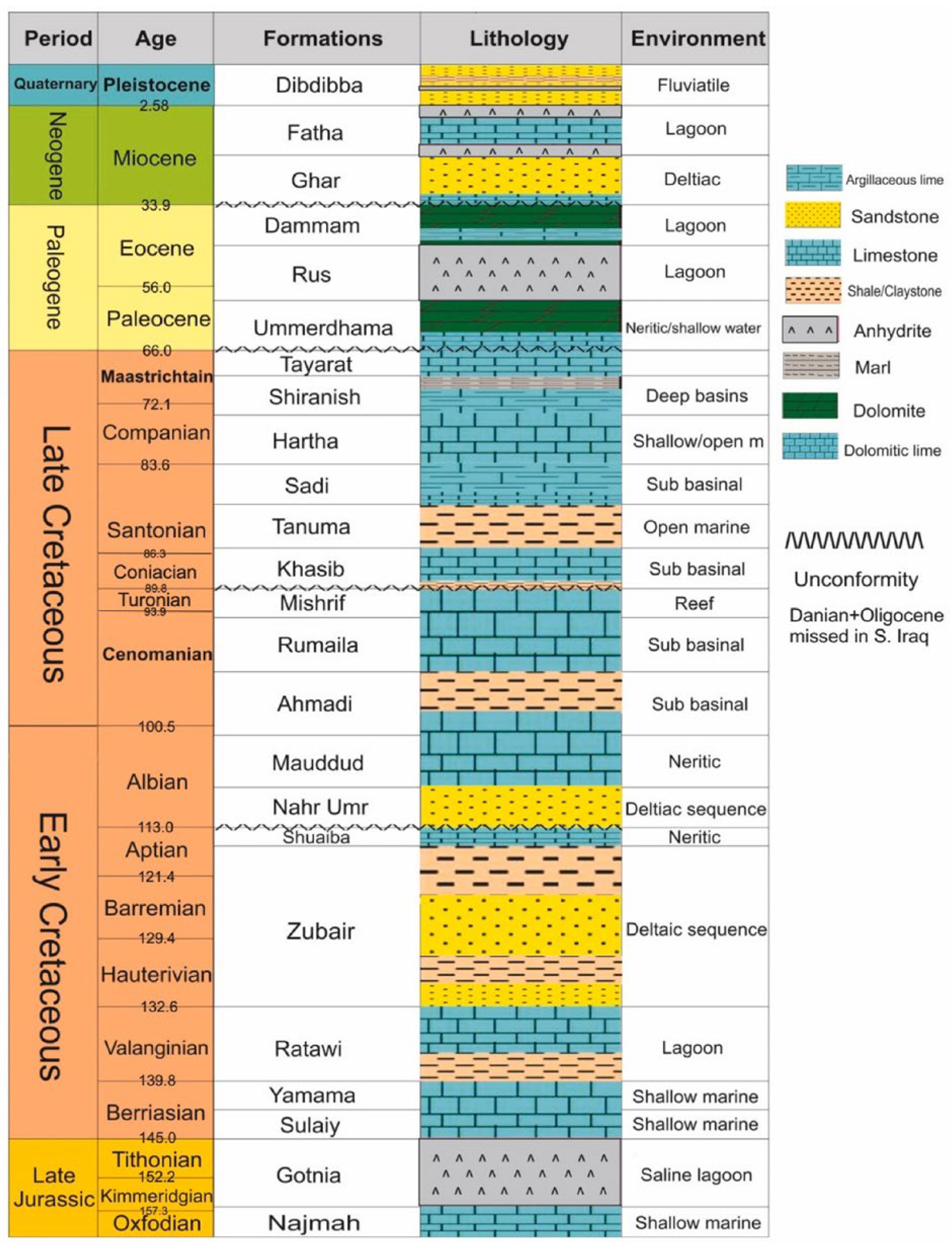The folded structures are characterized by their relatively narrow widths, extensive lengths spanning hundreds of kilometers, and separation by wider synclines [27]. The Early Cretaceous Zubair Formation serves as the primary reservoir in the South Rumaila Oilfield [33,34]. The Upper Sandstone Member, known as the Main Pay, is bounded by the Upper Shale Member above and the Middle Shale Member below (Figure 2). The Main Pay consists of three prominent sandstone units, AB, DJ, and LN, interbedded with two shale layers, C and K, which act as effective vertical seals for reservoir fluids, except in localized areas where these shale units are absent. From top to bottom, the units are as follows: AB (reservoir), C (shale), DJ (reservoir), K (shale), and LN (reservoir). The net thicknesses of the sandstone units are 9 m for AB, 55 m for DJ, and 41.5 m for LN. While AB is comparatively thinner than DJ and LN, its thickness and stratigraphic position make it an optimal target for horizontal drilling [26,27,28].

3. Methodology

3.1. Black Oil Model

The black oil model is a streamlined approach to reservoir fluid modeling that is extensively utilized in horizontal drilling and reservoir simulations. It defines reservoir fluids—oil, gas, and water—primarily by their volumetric properties rather than by detailed compositional analysis. This model is especially suitable for conventional reservoirs with limited compositional variability [35]. The black oil model assumes a three-phase system comprising oil, gas, and water, where gas can dissolve in oil, but oil does not vaporize into the gas phase. The model also applies Darcy’s law, modified to incorporate relative permeability for multiphase flow, with the assumption that no mass transfer occurs between the water phase and the other two phases. Dispersion effects are excluded from the model formulation, and the conserved quantities are expressed as stock tank volumes of oil, gas, and water. In this model, fluid flow through porous media is governed by the diffusivity equation, a partial differential equation that represents pressure and saturation as functions of both time and spatial coordinates.

In three-dimensional rectangular coordinates (x, y, z), the general equations for oil and water flow are expressed as follows [36,37]:

$${\displaystyle \frac{\mathsf{\partial }}{\mathsf{\partial }x}}\left[{\mathsf{\lambda }}_{lx}\left({\displaystyle \frac{\mathsf{\partial }{p}_l}{\mathsf{\partial }x}}-{\mathsf{\gamma }}_l{\displaystyle \frac{\mathsf{\partial }h}{\mathsf{\partial }x}}\right)\right]+{\displaystyle \frac{\mathsf{\partial }}{\mathsf{\partial }y}}\left[{\mathsf{\lambda }}_{ly}\left({\displaystyle \frac{\mathsf{\partial }{p}_l}{\mathsf{\partial }y}}-{\mathsf{\gamma }}_l{\displaystyle \frac{\mathsf{\partial }h}{\mathsf{\partial }y}}\right)\right]+{\displaystyle \frac{\mathsf{\partial }}{\mathsf{\partial }z}}\left[{\mathsf{\lambda }}_{lz}\left({\displaystyle \frac{\mathsf{\partial }{p}_l}{\mathsf{\partial }z}}-{\mathsf{\gamma }}_l{\displaystyle \frac{\mathsf{\partial }h}{\mathsf{\partial }z}}\right)\right]+q_l={\displaystyle \frac{\mathsf{\partial }}{\mathsf{\partial }t}}\left[\phi S_l{b}_l\right]$$

(1)

The derivative of the above equation and their details variables can be found in in the Supplementary Materials. The above equations were derived under the following assumptions: (1) Oil and water are compressible. (2) Permeability has three main vectors. (3) Flow occurs in three dimensions (x, y, z). (4) Compressibility of formation is included. (5) The flow is isothermal. Taylor’s series can be used to convert Equation (1) from a differential form to a finite difference form. Implicit pressure–explicit saturation (IMPES) was used to solve the above equations [36]. Eventually, the pressure equations will be

$$\Delta \left[T_w\left(\Delta P_o-\Delta P_{cow}-{\mathsf{\gamma }}_w\Delta D\right)\right]=C_{1p}{\Delta }_t{P}_w+C_{1w}{\Delta }_t{S}_w+Q_w$$

(2)

$$\Delta \left[T_o\left(\Delta P_o-{\mathsf{\gamma }}_w\Delta D\right)\right]=C_{2p}{\Delta }_t{P}_o+C_{2o}{\Delta }_t{S}_o+Q_o$$

(3)

3.2. Grid Construction

The current study utilizes a structured Cartesian grid-based black oil model [24] for sectorial simulation of the Rumaila Main Pay reservoir, employing a block-centered gridding approach with dimensions of 15 (x) × 11 (y) × 5 (z) cells, totaling 825 cells (584 active, 70.8%). The areal grid configuration features uniform cell dimensions of 1000 m (x-direction) and 866 m (y-direction), providing a total model footprint of 15,000 m × 9526 m, while the vertical discretization consists of five layers with variable thicknesses based on lithofacies units. To optimize computational efficiency, aquifer grids are excluded from finite-difference calculations and instead modeled analytically through source terms, following established practices [24]. Recognizing the importance of clear geometric representation, we enhanced Figure 3 to include (1) a 3D schematic of the grid structure distinguishing active/inactive cells, (2) cross-sectional views illustrating vertical heterogeneity, and (3) a plan-view map showing a real grid partitioning—collectively providing comprehensive visualization of the model architecture. This refined presentation ensures full transparency in grid construction while maintaining a balance between geological accuracy and numerical practicality.

3.3. Determination of Fluids Properties

Reservoir fluid properties, including viscosities, densities, and formation volume factors (FVF), are pressure-dependent. The reservoir fluids are assumed to be slightly compressible, with the reservoir oil being undersaturated. Under these conditions, the reservoir pressure exceeds the saturation pressure, maintaining a constant solution gas–oil ratio. The saturation pressure is approximately 2660 psi, compared to an initial reservoir pressure of 5186 psi measured at a depth of 3154.7 m below sea level. Studies by the authors of [38] confirm the presence of a uniform bubble-point pressure across the reservoir and consistent physical and thermodynamic properties for the oil in all Main Pay units. The following equations are applied to estimate the formation volume factor across grid block pressures under undersaturated reservoir conditions, the full derivation of the equation is provided in the Supplementary Materials:

$$B_o=B_{ob}/\left[1+C_o\left(P-P_b\right)\right]$$

(4)

where P_b = base or reference pressure; B_ob = oil FVF at base pressure; and B_o = oil FVF. These equations are derived from the general definition of compressibility. Shrinkage factor is easily obtained, since it is the reciprocal of FVF. A significant variation in pore volume with pressure has been assumed in the current simulator. In this study, an isothermal black oil model is developed, assuming that viscosity depends solely on pressure and is determined at reservoir temperature. The viscosity of water in both the reservoir and aquifer is considered constant, as it exhibits minimal dependence on pressure. To estimate relative permeability, capillary pressure, and oil viscosity—parameters available in tabulated form—a linear interpolation method is employed.

Reservoir fluid properties—such as viscosities, densities, and formation volume factors (FVFs)—are pressure-dependent and derived through laboratory measurements and correlations calibrated to South Rumaila field data. The oil phase is undersaturated, with an initial reservoir pressure of 5186 psi at a reference depth of 3154.7 m below sea level and a bubble-point pressure of 2660 psi. The oil FVF (B_o) ranges from 1.32 RB/STB (Stock Tank Barrel) at the bubble-point pressure to 1.28 RB/STB at initial reservoir conditions, as calculated using Equation (4) with a compressibility (C_o) of 5.2 × 10⁻⁶ psi⁻¹. The water FVF (B_w) is fixed at 1.02 RB/STB due to its minimal pressure sensitivity. Oil viscosity varies from 1.8 cP at the bubble-point pressure to 2.1 cP at initial pressure, while water viscosity remains constant at 0.5 cP.

3.4. Initialization

The initialization process involves defining the pressures and saturations for each grid block under initial conditions. In a state of static equilibrium, the phase velocities are zero, and the pressure gradients for each phase are governed by the hydrostatic head. The oil–water contact (OWC) represents the interface separating oil and water, where water saturation equals 1.0. When capillary pressure is significant, a transition zone forms above the water zone.

The calculation of the initialization can be summarized in the following steps [39,40]:

(1) Specifying a phase pressure (usually oil pressure) at a certain datum.

(2) Calculating oil pressure at the center of the blocks.

(3) Oil pressure at the oil–water contact.

(4) Water pressure at the oil–water contact is calculated from oil and capillary pressure.

(5) The pressure of water at the center of the blocks.

(6) After determining the oil and water pressure at the center of the blocks, capillary pressure at the center of the blocks can be determined.

(7) From capillary pressure-saturation data and using calculated capillary pressure, water saturation at the center of the block can be determined. Oil density is used in the above equations in the oil zone to calculate oil and water pressure, while in the water zone, the water density is used to calculate oil and water pressures.

The initialization process establishes pressure and saturation distributions across all grid blocks under static equilibrium conditions. The reference pressure is defined as 5186 psi at a datum depth of 3154.7 m. The oil–water contact (OWC) is positioned at 3269 m below sea level, featuring a capillary pressure transition zone with a thickness of 2.5 m. Initial saturations include an oil saturation (S_o) of 0.78 and a water saturation (S_w) of 0.22 within the oil zone, gradually increasing to 1.0 below the OWC. Capillary pressure behavior is modeled using Brooks–Corey correlations, employing an entry pressure of 12 psi and a pore-size distribution index of 2.1. The initialization workflow, detailed in steps 1–7 of Section 3.4, ensures alignment with field-measured data and is validated by an initial oil-in-place calculation of 6958 × 10⁶ STB, consistent with historical estimates.

3.5. Boundary Conditions

The current study used two types of boundary conditions, a no-flow boundary and a flow boundary [24]. The northern and southern boundaries are assumed to be of no-flow. The flow boundaries are east and west. The no-flow boundary is treated by specifying a reflection boundary to ensure no-flow across the regional boundaries.

3.6. Calculation of Transmissibility

Transmissibility is defined as the mobility of the phase divided by the formation volume factor of that phase.

This term is also called the flow coefficient. Mobilities must be evaluated at the boundaries separating adjacent grid blocks. The value of absolute permeability is usually assigned to the center of the blocks. In the current simulator, the kind of averaging is a harmonic meaning that is applied to the horizontal and vertical permeabilities. In the present simulator, single-point upstream weighting is used for approximating the interblock relative permeability. The direction of flow must be specified in order to determine the upstream grid block [24]. The phase formation volume factor, B, and the fluid viscosities are functions of pressure, and they are generally weak functions of space. In this study, upstream weighting is used to estimate the interblock formation volume factor. The interblock viscosity is approximated using midpoint weighting. The finite difference (discrete) transmissibility term resulted during the approximation of partial differential equations by the finite difference technique. For the three-dimensional problem, each grid block is surrounded by six grid blocks. Since flow may occur between grid blocks and their surroundings, six discrete transmissibility terms are required in the finite difference equation of a specified grid and phase. The unit of the calculated transmissibility is SCF/D-psi.

3.7. Calculation of Individual Production and Injection Rates for Vertical Wells

For the present problem, there are 42 production vertical wells that were opened to flow in the simulated domain during the simulation time of 51 years from 1954 to 2004. These wells are completed in many layers, and the production rate for each layer must be evaluated. This can be achieved by using the radial flow equation for pseudo steady-state pressure behavior. The equation of the oil flow rate is presented by [41]

$$Q_o=WI\left({\displaystyle \frac{K{K}_{ro}\Delta z}{{\mu }_o{B}_o}}\right)\left(P_b-P_{bh}\right)$$

(5)

For a well perforated in (J) grid blocks, the total flow rate is the sum of the rates for all the perforated intervals. The total flow rate can be distributed according to fluid mobilities by assuming that the difference in pressure between the wellbore and a grid block is the same for all blocks communicating with a given well. Good vertical communication can almost exist, regardless of the magnitude of k/k, due to the extremely small thickness of the reservoir relative to its areal extent [39].

$$Q_{oj}={\displaystyle \frac{{\left(K{K}_{ro}\Delta z/{\mu }_o{B}_o\right)}_j}{{\sum }_{j=1}^J {\left(K{K}_{ro}\Delta z/{\mu }_o{B}_o\right)}_j}}{Q}_o$$

(6)

Now, the rate of water production is given by

$${Q_w}_j={\left[{\displaystyle \frac{K_{rw}/\left({\mu }_w{B}_w\right)}{K_{ro}/\left({\mu }_o{B}_o\right)}}\right]}_j{Q}_{oj}$$

(7)

For water injection rates, there are 19 injection vertical wells in this reservoir, and the injection rate for each grid is estimated as follows:

$$Q_{wj}={\displaystyle \frac{K\Delta z{\left(\frac{K_{ro}}{B_o{\mu }_o}+\frac{K_{rw}}{B_w{\mu }_w}\right)}_j}{{\sum }_{j=1}^J {\left[K\Delta z\left(\frac{K_{ro}}{B_o{\mu }_o}+\frac{K_{rw}}{B_w{\mu }_w}\right)\right]}_j}}{Q}_w$$

(8)

3.8. Calculation of Individual Production Rates for Horizontal Wells

Four horizontal wells (HRU1, HRU2, HRU3, and HRU4) are assumed to be drilled from injection vertical wells (RU122, RU90, RU83, and RU162) because the injection of water was stopped in layers (DJ and LN) in the Main Pay formation of the South Rumaila Oilfield. The horizontal well (HRU1) is assumed to be open to flow at the beginning of the year 2008. The horizontal wells (HRU2, HRU3, HRU4) are assumed to begin production after 6, 12, and 18 months, respectively, from this date. The lengths of the horizontal wells HRU1, HRU2, and HRU3 are 2000 m, and the length of the horizontal well HRU4 is 1500 m. Figure 3 shows the location of the vertical and horizontal wells on the grid.

The production rate for each grid can be evaluated using the following equation [42]:

$$Q_o=PI{\displaystyle \frac{\underset{\_}{K}{K}_{ro}\Delta X}{{\mu }_o{B}_o}}\left(P_b-P_{bh}\right)$$

(9)

If the difference in pressure between the wellbore and a grid block can be assumed to be the same for all blocks communicating with a given horizontal well, the total flow rate can be distributed according to fluid mobilities. The water–oil ratio of horizontal well can be calculated by dividing the cumulative water production of grids that are penetrated by the horizontal well to cumulative oil production from those grids as follows:

$$WOR={\displaystyle \frac{\sum _{i=1}^1{Q}_{wi}}{\sum _{i=1}^1{Q}_{oi}}}$$

(10)

3.9. Calculation of Bottom-Hole Pressure of Horizontal Wells

In the current simulator, the bottom-hole pressure is determined for each perforated grid block completed by a horizontal well. The calculation is based on two key assumptions, as outlined by Intercomp [39]: (1) The viscous pressure losses in the wellbore are neglected. (2) The average density of the wellbore fluid is constant. Under these assumptions, the bottom-hole pressure at the center of any perforation is given by

$$P_{bhi}=P_{bh}^o+\overline{\mathsf{\gamma }} \left(D_i-D^o\right)$$

(11)

After the substitution of Equation (11) and rearrangement, the resulting equation for calculating flowing bottom-hole pressure opposite any perforation of grid block that is completed by horizontal well will be

$$P_{bhi}={\displaystyle \frac{PI{\sum }_{i=1}^I\left[{\left(\frac{\overline{K}{K}_{ro}\Delta x}{{\mu }_o{B}_o}\right)}_i\left\{P_{bi}-\overline{\mathsf{\gamma }}\left(D_i-D^o\right)\right\}\right]-Q_o}{PI{\sum }_{i=1}^I{\left(\frac{\overline{K}{K}_{ro}\Delta x}{{\mu }_o{B}_o}\right)}_i}}$$

(12)

3.10. Simulation of Aquifer

In this study, an unsteady state model simulates an aquifer by using the analytical solution of the diffusivity equation as developed by Van Everdingen and Hurst and modified by [43,44,45,46]. The influx rate for a specified grid block is estimated using the following equation:

$$Q_A=\alpha \left[A-B(P^{n+1}-P^n)\right]$$

(13)

where $P^n$ and $P^{n+1}$ are grid block pressures at the old- and new-time level, respectively. The terminal rate influence function can be estimated from the tables. The interpolation process is not used in the current simulator to estimate influence function because of the large storage requirement and lack of good accuracy. Hence, the analytical expressions for estimating the influence function proposed by Fanchi [44] are used in this simulator. The coefficient α represents the percentage of total water influx that invades each grid block. For the current problem, the water influx is distributed according to the grid block capacity (kΔz).

4. Results and Discussion

In this study, the simulation period was extended to 2004 to achieve a match between the average reservoir pressure and the well block pressure for vertical wells, based on available field pressure data. Additionally, the simulator was run for the period from 2008 to 2011 to estimate the average reservoir pressure, bottom-hole pressure, and water–oil ratio for hypothetical horizontal wells drilled in layer AB of the Main Pay reservoir in the South Rumaila Oilfield. The validity of the initialization results was evaluated using the black oil simulator by Hamad-Allah [24]. The saturation distribution was employed to calculate the initial oil in place, determined to be 6958 × 10 STB. The initial reservoir pressure was recorded at 5186 psi at a depth of 3154 m below sea level, with the water–oil contact located at 3269 m below sea level.

4.1. Average Reservoir Pressure

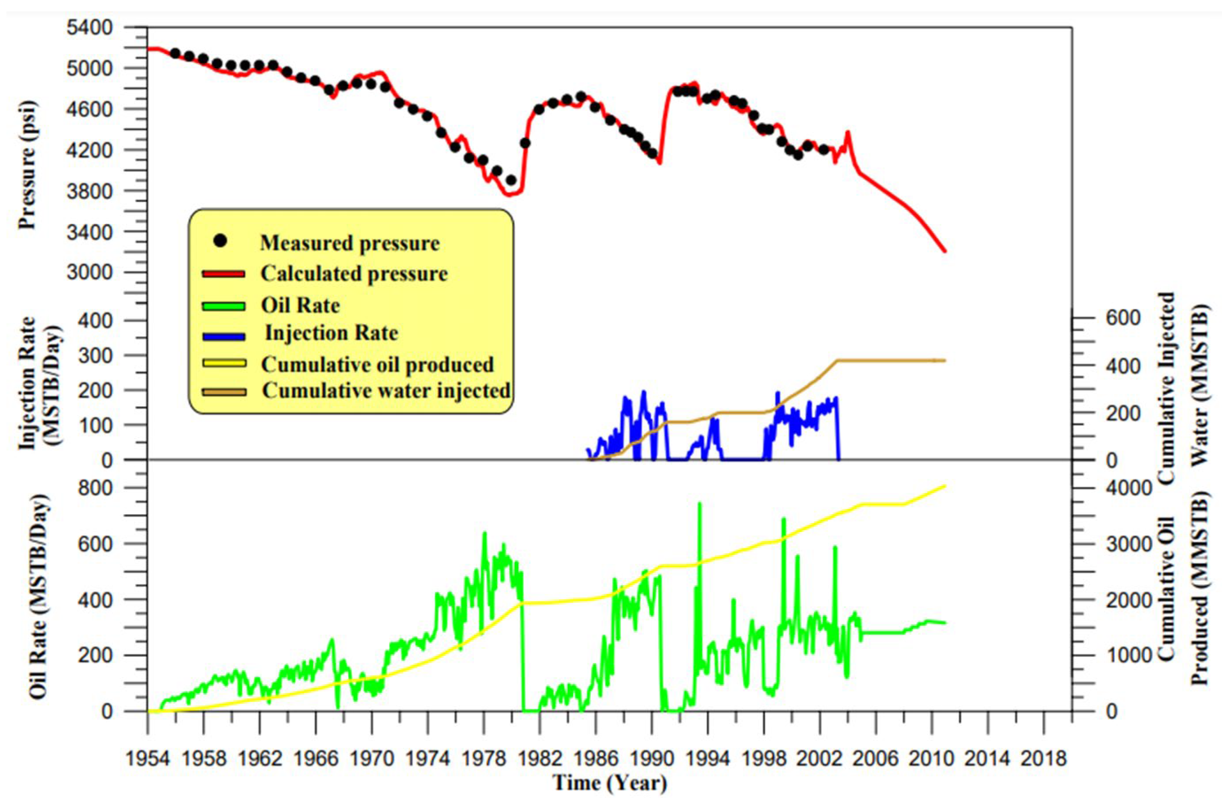
The current simulator is utilized to estimate the average reservoir pressure of the Main Pay reservoir. The results are presented in two parts. First, the calculated average reservoir pressure is compared with the measured values, as shown in Figure 4. A good match is achieved by applying a transmissibility factor of 0.5 and tripling the aquifer size on the eastern and western boundaries.

The selection of wells for analysis in this study was based on their strategic locations within the South Rumaila Oilfield, which capture diverse reservoir dynamics and boundary effects. Wells RU-2, RU-63, RU-46, and RU-75 were chosen to represent distinct geological and operational scenarios: RU-2 is near the eastern aquifer, RU-63 is crestal in the northern sector, RU-46 is in the far north with minimal boundary flow, and RU-75 is downdip on the western flank. This approach ensures a comprehensive evaluation of the simulator’s performance across varying reservoir conditions, including pressure responses, water influx, and production trends. The results from these wells collectively validate the model’s robustness and its ability to replicate observed field behaviors, making the analysis representative of the reservoir’s heterogeneity and operational challenges.

Second, the well block pressures for several wells are compared with the observed pressures, available only after 1980, as illustrated in Figure 5. The simulated well block pressures align well with the observed data, except in 1997, where discrepancies are attributed to measurement errors. Well Ru-2 is situated closest to the eastern aquifer, with its calculated and observed pressure history illustrated in Figure 5a. A good pressure match was achieved after 1980; however, discrepancies between calculated and observed pressures increased in 1988 and 1997. Well Ru-63, positioned near the crest in the northern part of the simulated domain, has its pressure and production histories, depicted in Figure 5b. Well Ru-46 is located in the far north of the simulated domain, and its pressure and production histories are shown in Figure 5c. The northern flow boundary is modeled as a no-flow boundary, a valid assumption due to minimal pressure discrepancies, except in 1997. Well Ru-75 is situated downdip on the reservoir’s western flank, with its pressure and production histories presented in Figure 5d, showing a good pressure match. Notably, the pressure discrepancies observed in 1997 (particularly the 8–12% deviation from modeled values in wells RU-2, RU-46, and RU-63) correlate with documented field instrumentation issues during that period, as recorded in the South Oil Company’s 1998 annual technical report [47]. The simultaneous occurrence of anomalous readings across multiple wells, coupled with their non-persistence in subsequent measurements, supports our classification of these as measurement artifacts rather than indicators of reservoir behavior.

4.2. The Results of Saturation

After the pressure calculations, saturation values were determined using the IMPES method. In layer AB, the difference between initial and final saturation distributions was minimal compared to layers DJ and LN. The greater water advancement observed in layer DJ is likely due to its higher production rate, which is attributed to its larger oil volume and higher permeability relative to other layers. The simulator results indicated increased water saturation in layers DJ and LN, driven by water injection at the eastern flank. Similar findings were reported by the South Oil Company/Reservoirs and Fields Development Directorate, prompting the decision to halt water injection at the eastern flank of the South Rumaila Oilfield.

4.3. The Results for Horizontal Wells

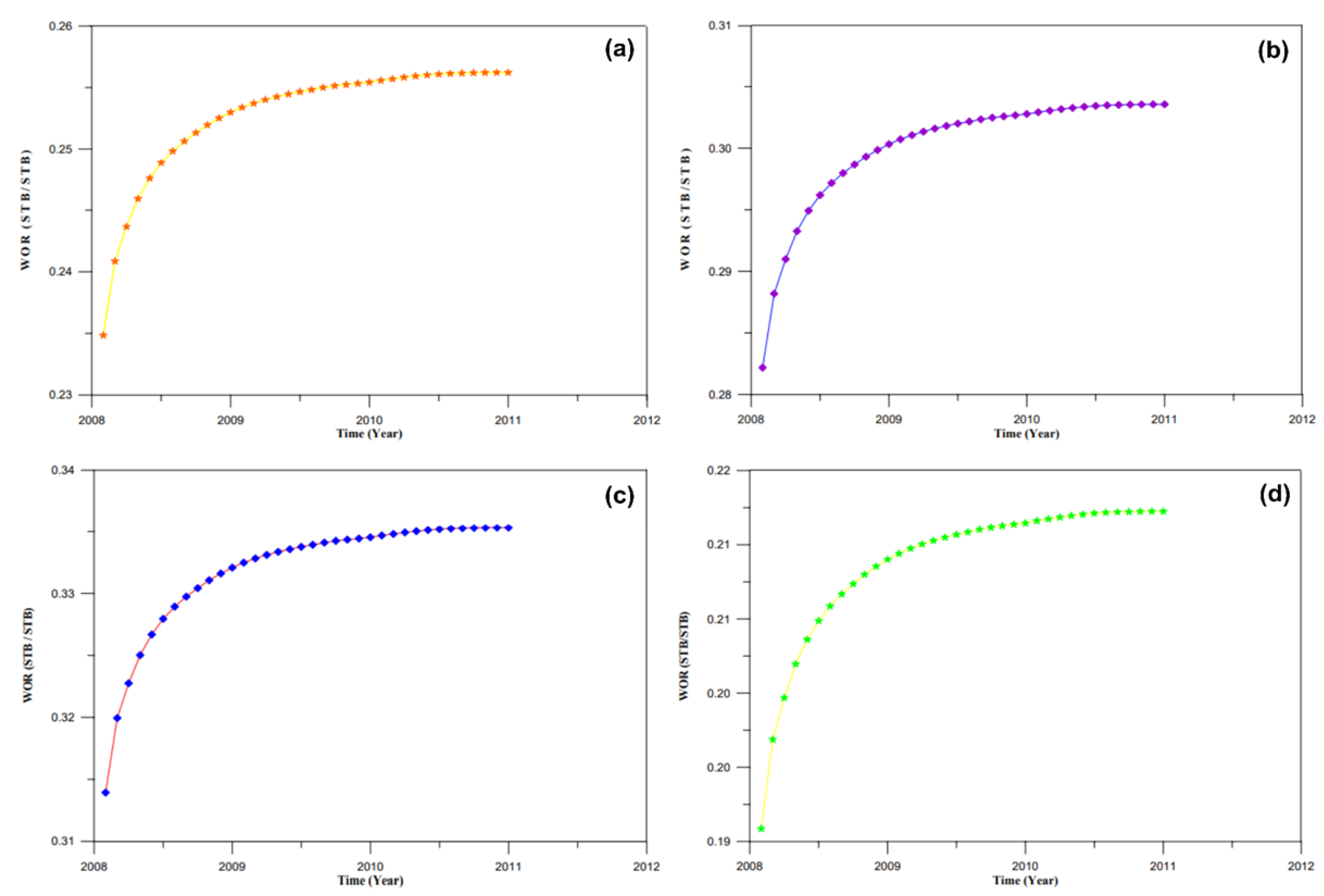
The simulator was applied to the South Rumaila Oilfield, incorporating four hypothetical horizontal wells. The simulation results include the average reservoir pressure, bottom-hole pressure, and water–oil ratio (WOR). It is assumed that no new vertical wells were brought into production after 2004. For the period between 2005 and 2011, the oil production rate for existing vertical wells is considered constant, matching the rate recorded at the end of 2004. Horizontal wells are assumed to begin production in 2008, with an initial rate of 11,000 STB/D for each well, except for the fourth horizontal well, which starts at 9000 STB/D. A decline in oil production is modeled at a rate of 100 STB/D per month. The water–oil ratio (WOR) results for each horizontal well are illustrated in Figure 6, while the bottom-hole pressure outcomes are presented in Figure 7.

The water–oil ratio (WOR) is defined as the ratio of cumulative water production to cumulative oil production from the grid blocks penetrated by a horizontal well. WOR calculations performed for HRU1 well (length = 2000 m) under various production rates of 11,000, 9000, and 7000 STB/day, with the results shown in Figure 8. A similar analysis was conducted for HRU1 with a reduced length of 1000 m. The results indicate that WOR decreases with increasing horizontal well length but rises with higher production rates. Doubling the horizontal well length results in a relatively small increase in flowing bottom-hole pressure. Conversely, increasing production rates leads to a negligible reduction in flowing bottom-hole pressure.

The omission of the gas phase in the mathematical model (Equations (1)–(3)) is justified by the specific reservoir conditions and assumptions of the Black Oil Model applied in this study. The South Rumaila Oilfield’s Main Pay reservoir is characterized by an undersaturated oil system, where the reservoir pressure (5186 psi) significantly exceeds the bubble-point pressure (2660 psi). Under these conditions, all gas remains dissolved in the oil phase, and no free gas phase exists. This aligns with the Black Oil Model’s assumption of a two-phase (oil–water) system for undersaturated reservoirs, where gas solubility in oil is accounted for via the solution gas–oil ratio (Rs) and oil formation volume factor (Bo), but explicit gas phase flow is negligible.

The model’s focus on oil–water flow is justified by the reservoir’s undersaturated state, where gas remains entirely dissolved in the oil phase. Historical data validation (Section 4.1) confirms that omitting explicit gas phase flow does not compromise the predictive accuracy for this system. For reservoirs with active gas caps or near-bubble-point conditions, additional phase modeling is required.

Our model achieves reliable forecasts with minimal computational resources, as demonstrated by the rapid convergence in pressure and saturation calculations (Figure 6 and Figure 7). Unlike generic commercial tools, our simulator integrates historical data from South Rumaila directly into its calibration, eliminating the need for extensive parameter tuning. The open-source framework (Visual Basic) reduces operational barriers for small-scale or mature field applications.

4.4. Limitations and Future Work

While this study demonstrates the simulator’s efficacy in modeling horizontal wells for the South Rumaila Oilfield, certain limitations warrant acknowledgment. First, the model assumes a two-phase (oil–water) system and excludes explicit gas-phase dynamics, which may restrict applicability to reservoirs with significant gas caps or volatile oils. Second, aquifer interactions are modeled analytically rather than via full hydrodynamic coupling, potentially simplifying boundary effects in highly heterogeneous settings. Third, calibration relied solely on South Rumaila field data; validation across geologically diverse basins would strengthen generalizability. Finally, computational optimizations prioritize accessibility over high-resolution capabilities (e.g., complex fracture networks).

To address these constraints, future work will

• Expand model physics to incorporate three-phase flow and compositional effects for volatile oil/gas condensate systems;
• Conduct rigorous benchmarking against established commercial simulators (e.g., CMG, Eclipse) to quantitatively assess predictive accuracy across reservoir types;
• Integrate machine learning for automated history matching and uncertainty quantification;
• Extend validation to carbonate and unconventional reservoirs with real horizontal well production data.

These enhancements will solidify the simulator’s versatility while retaining its core advantages: computational efficiency, open-source accessibility, and field-specific customization.

5. Conclusions

The results of the present simulation study lead to the following key conclusions:

• Model Validation: The simulator demonstrated robust performance, achieving a consistent match with observed data throughout the simulation period across various production scenarios in the Main Pay reservoir within the Rumaila sector of the South Rumaila Oilfield. This highlights the reliability and applicability of the simulation approach employed in this study.
• Effect of Horizontal Well Length on WOR: Increasing the length of horizontal wells effectively reduces the water–oil ratio (WOR) to a constant flow rate, indicating enhanced production efficiency. However, a significant increase in the flow rate results in only a marginal rise in WOR.
• Impact on Bottom-Hole Pressure: The flowing bottom-hole pressure for horizontal wells increases with greater length, while higher flow rates lead to a reduction in pressure. Notably, for the given reservoir conditions, well lengths, and flow rates, the pressure reduction remains negligible, underscoring the suitability of horizontal drilling strategies for optimizing reservoir performance.
• Relevance to Resource Accessibility and Extraction Efficiency: By optimizing configurations and flow rates, this study contributes to more efficient hydrocarbon extraction while minimizing water production and maintaining reservoir stability. The insights gained can help reduce operational costs, extend the productive life of reservoirs, and support strategic planning for field development. These outcomes are directly aligned with improving the accessibility and sustainable extraction of subsurface resources.

These findings reinforce the advantages of horizontal well technology in enhancing production efficiency while maintaining reservoir integrity, providing valuable insights for reservoir management and field development planning.