Assessment of Aerodynamic Plates Subjected to Von Kármán Vortex Street for Enhancing the Wind Energy Generation in Blade-Less Devices

Abstract

This study explores the feasibility of using an oscillating plate downstream of a cylindrical body to produce mechanical energy from a Von Kármán vortex street under sub-critical flow conditions (Re = 72,500). The study aims to quantify the impact of the plate length, its separation from the cylinder, and a machine damping factor on the power coefficient and the blade’s displacement to identify the optimal configuration. This preliminary assessment assumes that the plate oscillation is small enough to avoid changes in the vortex dynamics. This assumption allows the construction of a surrogate model using Computational Fluid Dynamics (CFD) to evaluate the effect of plate length and separation from the cylinder on the fluctuating lift forces over the plate. Later, the surrogate model, combined with varying machine damping factors, facilitates the description of the device’s dynamics through the numerical integration of an angular momentum equation. The results showed that a plate with a length of 0.52D, a separation of 5.548D from the cylinder, and a damping factor of 0.013 achieved a power coefficient of 0.147 and a perpendicular displacement of 0.226D. These results demonstrate a substantial improvement in the performance of blade-less generators.

1. Introduction

Wind generators are machines commonly implemented to transform the kinetic energy of wind into electricity through sustainable and efficient processes. Among the available technologies in the field, horizontal devices are popular due to their high power coefficient (able to transform more than 40% of the wind’s kinetic energy). Therefore, this type of generator accounts for 12% of the worldwide electrical energy production, contributing to a production of 1100 GW by 2020 [1].

Although horizontal wind turbines have a high power coefficient, researchers and manufacturers are also exploring small-scale wind turbines to produce electricity in remote regions, considering essential factors such as low complexity in manufacturing, low maintenance costs, small size, and low noise. These factors are achievable with small-scale wind turbines. Figure 1 shows some of these options, including the Savonius turbine and the Darrieus turbine, which are vertical-axis wind turbines.

According to Figure 1, it is easy to see that the energy extraction from wind mainly comes from devices that transform mechanical energy into rotating shaft work. However, novel options that convert kinetic energy into oscillating mechanical work are gaining interest in the scientific community. These apparatuses are commonly known as blade-less generators [3].

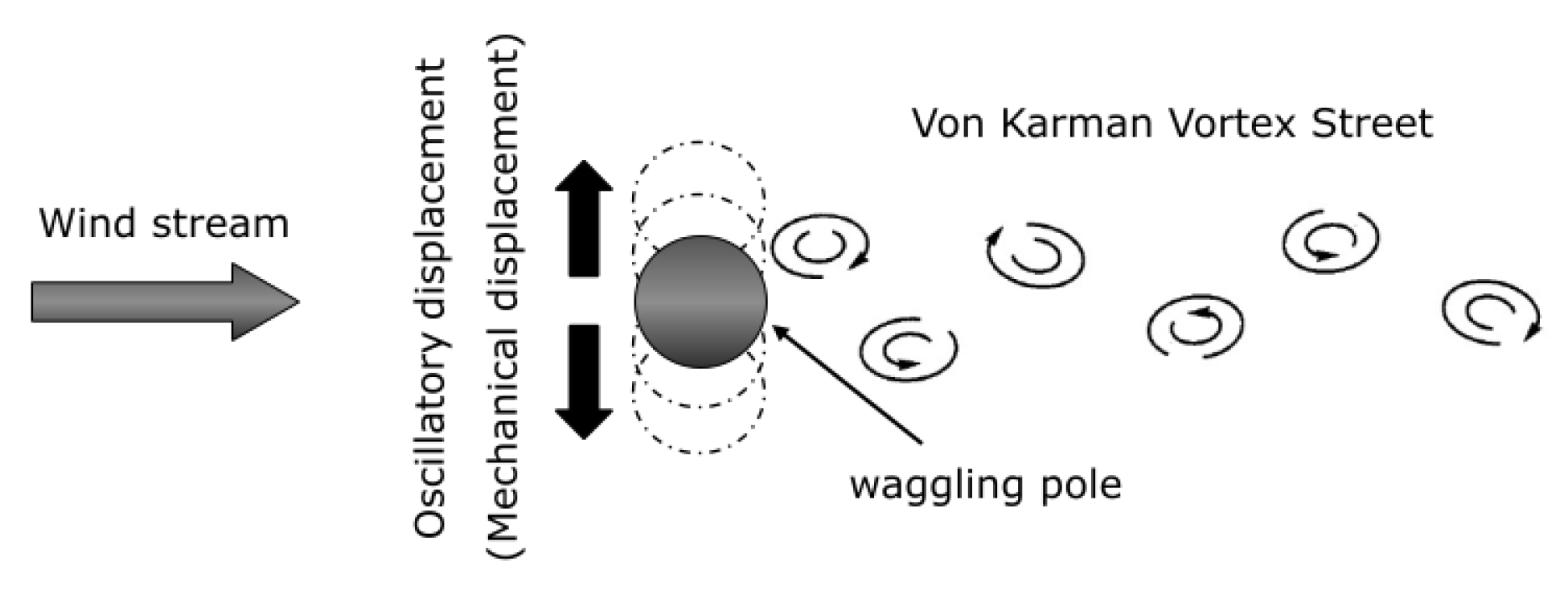
Figure 2 illustrates a schematic depiction of blade-less generators, characterised by cylindrical or conical poles that generate a Von Kármán vortex street when wind crosses them. The Von Kármán vortices have the potential to produce vibrations in these poles through an aero-elastic resonance of their structure, later on converted into electricity using magnetic induction [3].

Different experiments and CFD analyses have addressed the study of these types of machines; for example, the work of [4,5,6,7,8,9,10]. Moreover, Yáñez [3] introduced two commercial devices, the Vortex Nano and Vortex Tacoma, to the market. According to Ordoñez et al. [11], Nano can generate 0.9 W of power when a prototype 0.85 m in height is 8 m above ground level, exposed to a wind speed of 6.5 m/s, while Tacoma can generate 110 W with a wind speed of 9 m/s. They [11] also projected that a generator with a height of 2.75 m could transform 30% of the wind energy into electrical work, representing an appropriate increment in conversion efficiency.

Apart from the design of Yáñez [3], some researchers have studied configurations that include bulk or aerodynamic shapes at the rear of a rigid pole to exploit the vortex energy at the wake zone. For example, Eldredge and Pisani [12] studied the aerodynamic behaviour of three bodies exposed to a Reynolds number of 100, demonstrating that vortices can produce work in a stable process depending on the dimensions of the bodies. Wu and Shu [13] simulated the alterations in the dynamics of vortices in a flow with low Reynolds Numbers (Laminar condition) caused by different plates placed downstream on the pole. This study found that the motion and length of the plate were factors capable of modifying the flow structures of the wake behind the cylinder. Wang et al. [14] studied the behaviour of aerodynamic surfaces in a test bench that could adjust the distance of these surfaces from a cylindrical body and their stiffness. This experiment reported an optimal separation of three to four times the cylinder diameter for a fluid with a Reynolds Number between 100 and 200, as the authors explain that this ensures an appropriate development of vortices, enabling a complete interaction with the plate.

Mojra and Abdi [15] delve deeper into controlling the vortex-induced vibration (VIV) phenomenon by implementing flexible and rigid plates in a flow regime of Re = 100. Using a methodology based on CFD and parametric analysis, the authors determined that plates in the wake zone are a very effective passive method to suppress vortices (especially when using rigid plates). Alongside this, they establish that the inclusion of plates could also be promising for power generation using piezoelectric materials. Finally, Lee et al. [16] evaluated the fluid-dynamic behaviour and the energy generation capacity of tandem cylinders under Reynolds number values of 3790, 8470, and 15,610. This research considered two operational scenarios, one in which the cylinder in the wake zone describes a translational motion and the other where the cylinder describes a pendular movement with a rotational centre at the fixed vortex-generating cylinder. As a result, drag is reported to increase the oscillation frequency because it acts as an additional restoring force. In addition, the study found that the pendulum motion system had a higher efficiency of 1.7–3.7% compared to the translational motion system.

Given the above, the present work aims to study the impact of Von Kármán vortex street on a plate downstream of a rigid cylinder (pole) to harness vortex energy in the wake zone. The study employs a multi-objective optimisation approach to determine the plate length and distance from the cylinder that maximises the power coefficient of the device while minimising its oscillation amplitude. The plate length varies between 0.5D and 1D, while the cylinder-plate separation ranges from 1D–7D. The evaluation considers a Reynolds number of 72,500, as Norberg [17] reported high values of lift coefficient on circular cylinders at this condition.

2. The Studied Problem: Device’s Structural Dynamics Responses

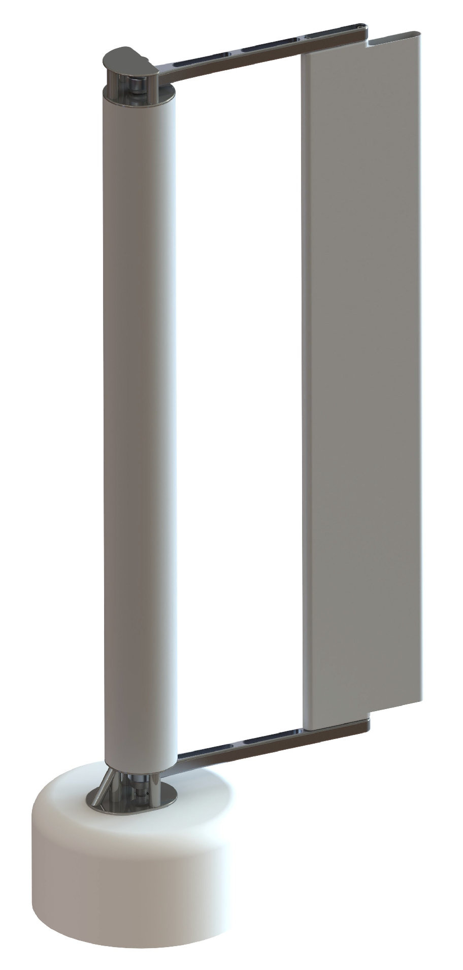
The studied wind-generator concept involves a plate with a single degree of freedom oscillating along an axis aligned with the length of an upstream-placed cylinder. The oscillation occurs due to a fluctuating lift force on the plate, which appears when the plate interacts with the wake generated by the cylinder on a crossing fluid. Finally, the lift force creates torque with a fluctuating angular velocity, which turns into electricity through magnetic induction. Figure 3 shows a model of the whole device.

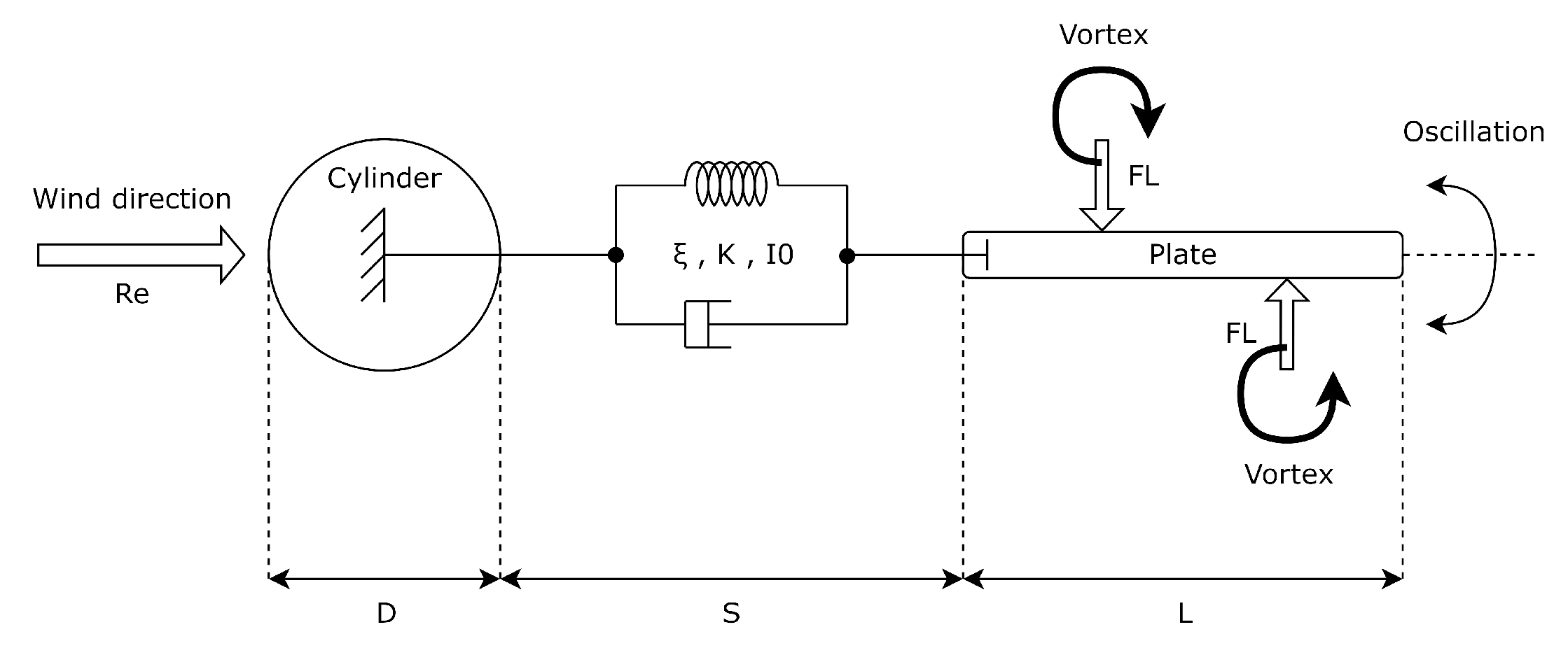
The fluctuating lift force on the plate, which favours its vibration, depends on the cylinder-plate separation (S), plate length (L) and the dynamics of the Von Kármán vortex street. Its study, therefore, requires either laboratory tests or the application of CFD. Additionally, Newton’s second law of motion in a rotational framework governs the response of this vibrating system to external driving forces $F_L$, for known values of the damping factor $\xi$, restoration forces K, and the body inertia $I_0$ [18]. Therefore, the maximum power conversion of blade-less devices occurs under their resonance conditions. Figure 4 shows a simplified representation of the device configuration and the interaction of vortices.

3. Methodology

The following methodology presents a process that includes the development of a surrogate model to account for the fluid-dynamic effect on the lift coefficient over a plate, the construction of a structural-dynamic model capable of linking material properties and the surrogate model with the power coefficient and angular displacement of the device, and the execution of an optimisation process. The following subsections present an in-depth discussion of each part of the proposed methodology.

3.1. Studied Variables

The dynamic behaviour of the studied configuration is a function of multiple variables, commonly expressed as non-dimensional quantities. This work centres its attention on four of them for a fixed Reynolds Number, as follows:

3.1.1. The Lift-Coefficient

It is a non-dimensional parameter widely used in aerodynamic profiles. This value measures the ratio between the lift force (parallel to the flow direction) and a force derived from the dynamic pressure.

Equation (1) allows computing the Lift-Coefficient, where $F_L$ is the lift force, $V_{\infty }$ is the free-stream velocity magnitude, $\rho$ is the fluid density, and s represents a surface area of reference. A suitable blade-less generator must assure a high value of this amount.

$$Cl=\frac{F_L}{\frac{1}{2}\rho {V_{\infty }}^{2}s}$$

(1)

When working with discrete values, such as laboratory measurements or transient CFD results, the non-dimensional lift coefficient is expressed as a root mean square (RMS) value ($C{l}^{\prime }$) computed during a specific time interval. Equation (2) gives the mathematical expression of ($C{l}^{\prime }$), where i represents a discrete value out of n data points.

$$C{l}^{\prime }=\sqrt{\frac{1}{n}\sum _{i=1}^n{C{l}_i}^2}$$

(2)

3.1.2. The Strouhal Number

It describes the ratio between a characteristic flow time and an oscillation period. This parameter allows describing the Von Kármán vortex frequency. Equation (3) represents the Strouhal number, where f is the vortex shedding frequency, L is the characteristic length, and $V_{\infty }$ is the free-stream velocity magnitude.

$$St=\frac{fL}{V_{\infty }}$$

(3)

The vortex-shedding frequency comes from a discrete form of the Fast Fourier Transform (FFT). Equation (4) gives the FFT discrete format implemented during the assessment, available in the SciPy library [19]. In this equation, $Cl\left[n\right]$ denotes the N-periodic signal data, $e^{-2\pi j\frac{kn}{N}}$ is the primitive nth root of unity, k is the integer frequency, n is the index of a data point, and N is the total number of data points of the discrete signal. Rao and Yip [20] present an in-depth study of the subject.

$$y\left[k\right]=\sum _{n=0}^{N-1}C{l}_{\left[n\right]}{e}^{-2\pi j\frac{kn}{N}}$$

(4)

3.1.3. The Perpendicular Displacement

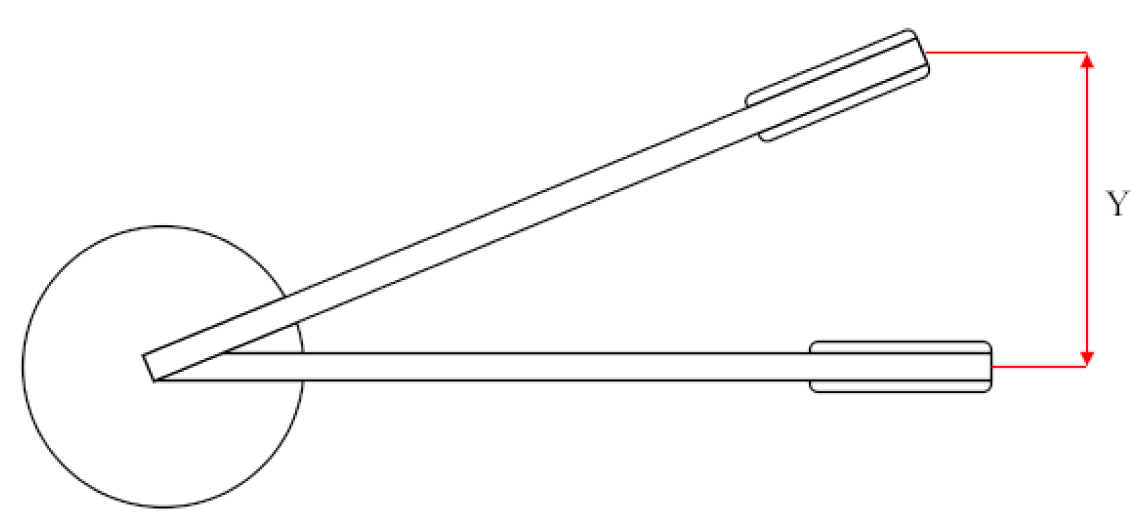
It is a dimensionless variable implemented in this study to quantify changes in the device’s relative position (in this case, the plate of the wind generator) according to its neutral position and the cylinder diameter D. Figure 5 helps describe this variable, denoted by Y.

3.1.4. The Power Coefficient

It is a non-dimensional number that allows computing the amount of power that wind generators can withdraw from the wind according to Equation (5). Therefore, this number emulates the conversion efficiency of a wind generator [21]:

$$Cp=\frac{{\dot{W}}_{generator}}{{\dot{W}}_{available}}=\frac{{\dot{W}}_{generator}}{\frac{1}{2}\rho {V_{\infty }}^{3}A}$$

(5)

3.2. The Surrogate Model

Figure 6 shows the developed methodology at this stage. The subsequent subsections describe the procedures followed by this work.

3.2.1. CFD Model

This work implements the CFD software SimScale to compute the solution of the underlying differential equations. SimScale is a computer-aided engineering (CAE) software based on cloud computing that uses OpenFOAM at its core.

The simulation of Von Kármán’s Vortex streets requires complex turbulent models capable of predicting the vortices oscillation according to the order of the Reynolds number set in this study. Large Eddy Simulation (LES) is a suitable option for the task because it offers accuracy with a reasonable computational cost. LES computes large eddies and their interaction to represent the Von Kármán Vortex’s dynamics while minimising the processing time by including a sub-grid filter to model small eddies.

Equation (6) represents the tensorial notation of the momentum equation of incompressible flow commonly solved by CFD codes centred on the LES model [22]. The terms on its left denote the transient behaviour of the control volume and the momentum fluxes. In addition, the ones on its right represent the contribution of any pressure gradient and the viscous stress tensor, which includes the sub-grid stress tensor (${\tau }_{ij}$). The purpose of the sub-grid stress tensor is the artificial dissipation of eddies larger than the domain cell sizes.

$$\begin{array}{c}\hfill \rho \left(\frac{\partial }{\partial t}{\underline{u}}_i+\frac{\partial }{\partial x_j}\left({\underline{u}}_i{\underline{u}}_j\right)\right)=\frac{\partial }{\partial x_j}\left(\frac{\partial {\underline{\sigma }}_{ij}}{\partial x_i}\right)\\ \hfill -\frac{\partial \underline{p}}{\partial x_i}-\frac{\partial {\underline{\tau }}_{ij}}{\partial x_j}\end{array}$$

(6)

Equation (7) defines the sub-grid scale stress ${\underline{\tau }}_{ij}$. This equation includes ${\mu }_t$ as the subgrid-scale eddy viscosity, ${\underline{S}}_{ij}$ as the resolved scale rate of the strain tensor, ${\underline{\tau }}_{ij}$ as the isotropic part of the sub-grid scale stresses, and ${\underline{\sigma }}_{ij}$ as the stress tensor due to molecular viscosity [22].

$${\underline{\tau }}_{ij}=\frac{1}{3}{\underline{\tau }}_{kk}{\delta }_{ij}-2{\mu }_t{\underline{S}}_{ij}$$

(7)

Different options allow for the calculation of ${\mu }_t$. This work makes use of the Smagorinsky–Lilly model for homogeneous isotropic turbulence. On the one hand, the Smagorinsky–Lilly model is simple, easy to implement, and computationally inexpensive [23]. Moreover, OpenFOAM includes a well-developed library of this option.

Equation (8) shows the subgrid-scale eddy viscosity ${\mu }_t$ of the Smagorinsky–Lilly model according to the OpenFOAM documentation [22]. In this equation, $C_s$ is the Smagorinsky coefficient, set equal to 0.094 [24], $L_s$ represents the mixing length for sub-grid scales, and $\left|\underline{S}\right|$ is equal to $\sqrt{2{\underline{S}}_{ij}{\underline{S}}_{ij}}$.

$${\mu }_t={\mu }_{sgs}=\rho {L_s}^2{C_s}^2\left|\underline{S}\right|$$

(8)

An in-depth discussion about this topic is presented by [25,26].

3.2.2. Model Setup

The model setup follows the SimScale validation tutorial titled “Large Eddy Simulation of Flow Over a Cylinder” [27], but with changes that ensure a Reynolds number of 72,500, as described in

Table 1. Fluid Properties.

Fluid	Air
$\rho$ ($\frac{\mathrm{kg}}{{\mathrm{m}}^3}$)	1.145
Dynamic Viscosity $\left(\frac{\mathrm{kg}}{\mathrm{ms}}\right)$	1.1895 $\times {10}^{-5}$

,

Table 2. Boundary conditions.

Name	Type
Inlet	$4\frac{\mathrm{m}}{\mathrm{s}}$ normal direction (free stream)
Outlet	Gauge pressure 0 Pa
Cylinder	Wall
Others	Symmetry

and

Table 3. Numerical settings.

Name	Type
CFD Model	LES 3D
Algorithm	PISO
Numerical Scheme	2nd Order Upwind
Sub-Grid Scale Model	Smagorinsky-Lilly
Time step	$2.5\times {10}^{-4}$ s
Flow time	12 s

.

The time step of the model varies based on the Courant number. The latter is limited to a range between $0.7$ and $0.8$. In addition, the sampling frequency used to calculate the RMS lift coefficient and the Strouhal number corresponds to 10 time steps.

3.2.3. CFD Vortex Shedding Validation

The Von Kármán Vortex Street gets strongly connected to the vortex shedding on the bluff body surface. Therefore, the CFD simulation must guarantee the adequate modelling of the boundary layer around the body. Accordingly, a mesh whose resolution ensures an appropriate aspect ratio of the cells near the bluff body and an adequate number of layers along any radial projection from this body is necessary. As a strategy to reach the goal, this work assures the following:

• Mesh selection came from a validation process that reduced the discrepancy between the RMS lift coefficient and the Strouhal number predicted by the CFD simulation and the experimental values given by Norberg [17].
• The mesh implements an approach that defines the height of the first cell of the boundary layer to assure a $y^{+}$ lower than 1 [28], using the skin friction coefficient approximation from the author of [29]. The height value of the first cell attached to the wall is $5\times {10}^{-5}$ m, which represents 62% of the value predicted by the mentioned correlation.

Additionally, the mesh considers the appropriate trend of the kinetic energy spectrum solved by the model on probe points located 1D and 1.5D downstream from the cylinder mesh. The latter ensures the mesh’s capability to solve the turbulent kinetic energy, as these probe measurements described a slope of −5/3 following the Kolmogorov theory [26].

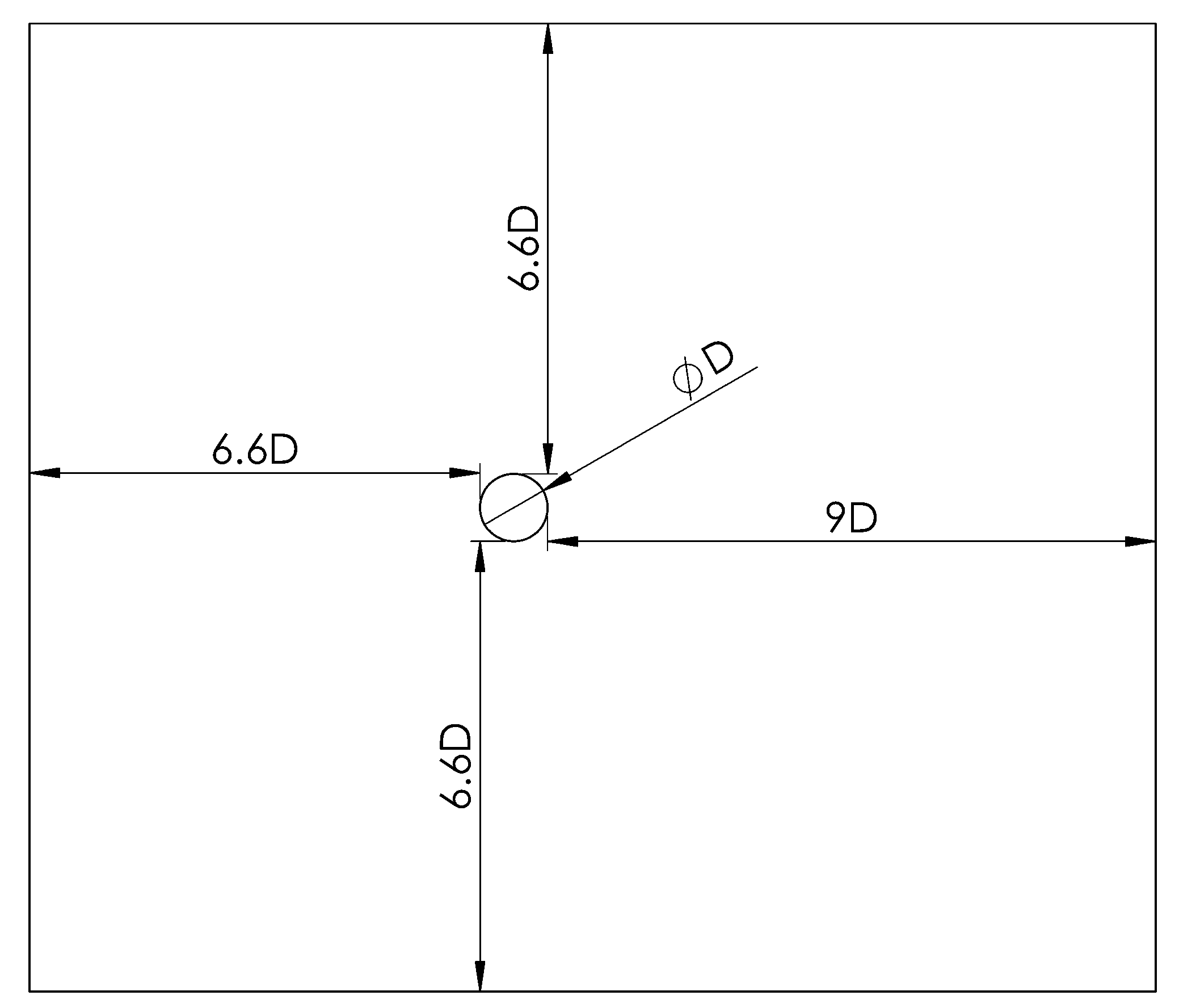
The validation case considers a 3D simulation of an open flow condition where a fluid stream crosses a cylinder of 0.3 m in diameter, reaching a Reynolds number equal to 72,500 (see Section 1). Figure 7 represents the side view of the evaluated domain, whose dimensions depend on the cylinder diameter (D), including its depth, which is three times the cylinder diameter (3D), as recommended by Cao and Tamura [30], with a number of 15 divisions of the mesh.

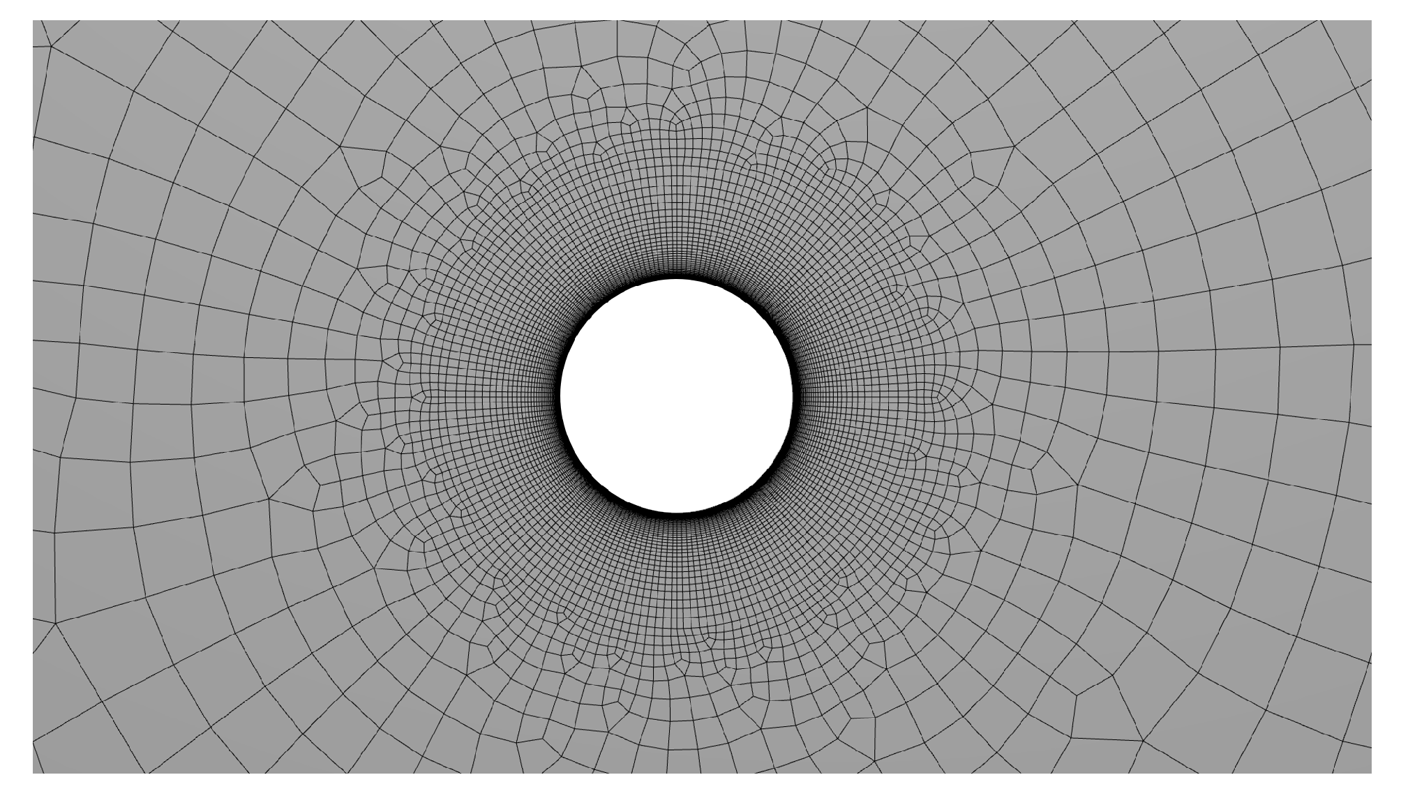
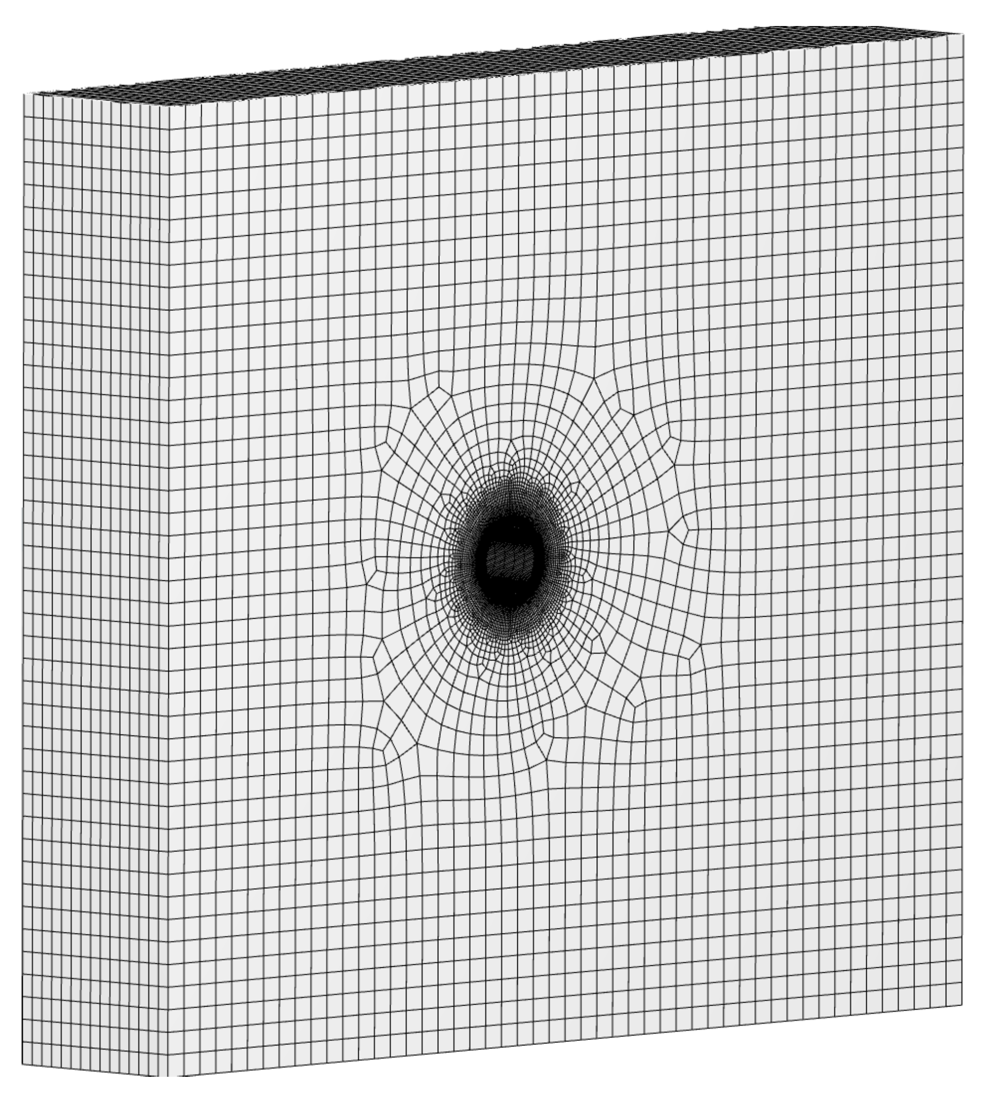
Figure 8 shows the discretisation of the domain in the vicinity of the cylinder. The implemented mesh has non-structural hexahedral elements and prismatic cells near the wall. Moreover, the discretisation assures a maximum aspect ratio of 100 near the cylinder and a growing factor of 1.2. Figure 9 shows the 3D mesh in an isometric view.

3.2.4. Latin Hypercube Sampling (Design of Experiment)

Engineers commonly use LES for the CFD evaluation of turbulent flow, thanks to the evolution of modern computers, which allows increasing the number of cells implemented during the domain discretisation while keeping a reasonable time for running the studied cases. However, its implementation in optimisation, although possible [31], is still a challenge, as the processing time applies to various configurations to trace the search path toward the optimum condition. A common alternative to overcome this issue involves the design of experiments (DoE) with a limited number of simulations, N, but enough for constructing a surrogate model to predict the response of the studied variables in locations different from the samples evaluated using CFD [32].

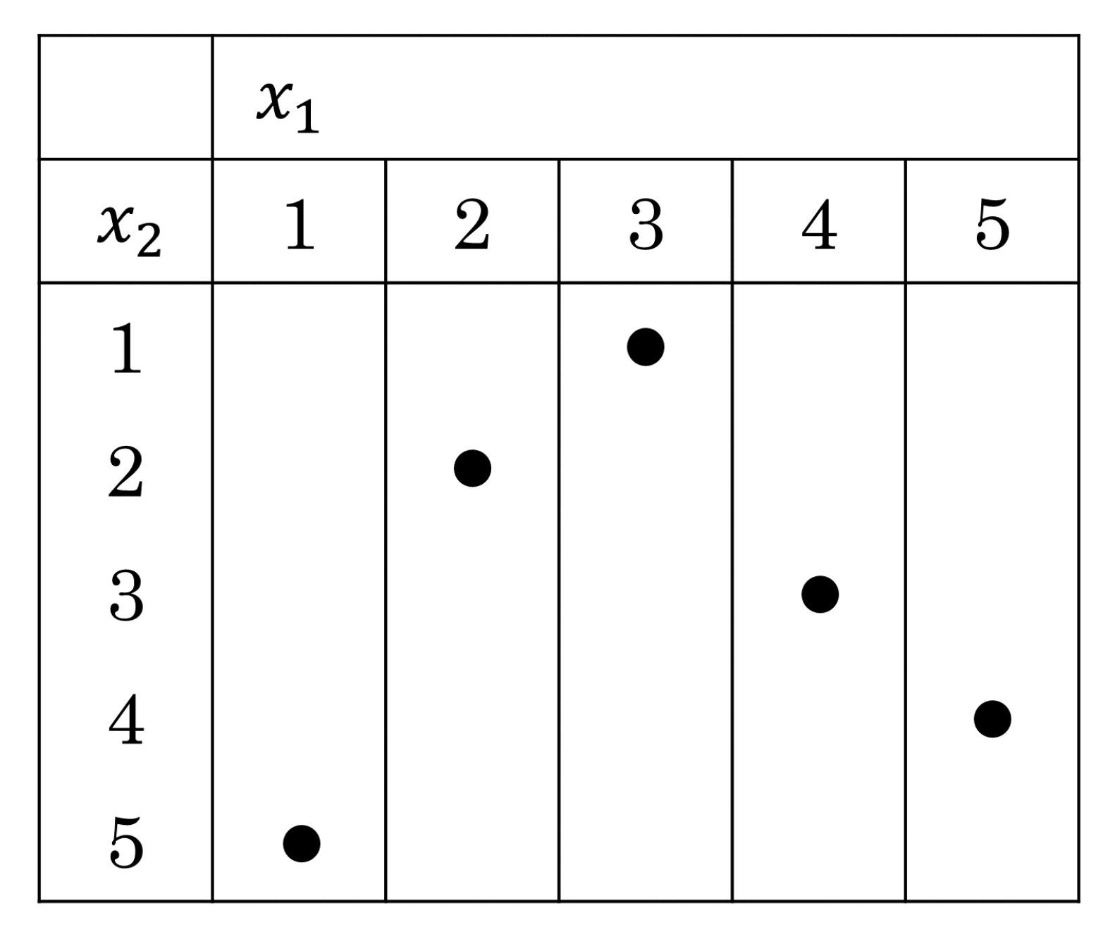
The dataset that allowed this work to build the surrogate model comes from a Latin Hypercube sampling (LHS) of two independent variables, L and S. In this method, the built square grid contains only a sample in each row and column. The evaluation range of each variable is divided into equal intervals to obtain the same number of sample points for each variable (see Figure 10) [33].

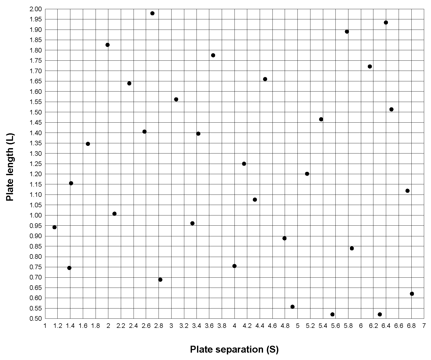
In this study, S changes between 1D ≥ S ≥ 7D and L between 0.5D ≥ L ≥ 2D. The plate width is 0.2D, and the initial size of the sampling is 15 points per variable, a value above the minimum number recommended by Kleijnen [32].

3.2.5. CFD—Cylinder Plate Evaluation

For the cylinder-plate cases, the domain suffers modifications because of the addition of the plate. However, the new mesh preserves the same characteristics defined in the vortex shedding validation process near the cylinder by keeping a growth ratio of 1.2 across the domain walls and a better aspect ratio. All of this assures a good prediction of the boundary layer.

Figure 11 shows the parametric dimensioning of the CFD domain according to the diameter of the cylinder (D), where S is the distance between the plate and the cylinder, and L is the plate length. In addition, the width of the domain (direction normal to the section shown in Figure 11) is three times the diameter of the cylinder (3D), as recommended by the authors of [30].

3.2.6. Surrogate Model and Vortex Shedding Suppression

Among the mathematical functions available to build a surrogate model, radial basis functions have a track record in the field. Their general format contains a constant term $\mu$ and a localised deviation $M\left(x\right)$ that considers the sampling data from the design of experiments [34] (see Equation (9)).

$$y\left(x\right)=\mu +M\left(x\right)$$

(9)

This work applies a Kriging interpolation function, constructed from the dataset evaluation using CFD, to predict configurations that maximise the RMS lift coefficient of an aerodynamic plate positioned downstream of a cylinder. $M\left(x\right)$ in the Kriging Model handles the covariance of the sampling ${\sigma }^2$ and a correlation function derived from it. Different codes are available to construct the Kriging Model, but in this case, the results come from a Python code developed by PyKrige. Kleijnen and Simpson et al. [32,34] present an in-depth description of the Kriging interpolation function, while Murphy et al. [35] offers a description of the Python library. Finally, the surrogate model implements an exponential variogram model for a 300 × 300 grid size, which allows obtaining an output field of 90,000 points to evaluate the objective functions.

Equation (10) enables the measurement of the surrogate model’s accuracy; it arises from the leave-one-out cross-validation (LOOCV) strategy. This equation utilises a normalised root-mean-square error ($NRMSE$) of the model’s predictions, where $\widehat{y}$ represents the predicted response, y denotes the actual value, and i is a sample from the available universe of n samples. Additionally, $y_{max}$ and $y_{min}$ are the maximum and minimum values of y, computed from the sampling points after their CFD evaluation.

$$NRMSE=\frac{\sqrt{\frac{{\sum }_{i=1}^n{\left({\widehat{y}}_i-y_i\right)}^2}{n}}}{\left(y_{max}-y_{min}\right)}$$

(10)

The Kriging interpolation function is appropriate for predicting variable responses under different conditions. Nevertheless, this is only possible if objective functions behave like continuous functions through the design space. Unfortunately, the experiment results can describe some discontinuities because of an instantaneous zero-lift condition when the aerodynamic surface gets closer to the pole since it can break the vortex dynamics, a phenomenon known as vortex shedding suppression, reported by the authors of [36,37].

Based on the above, a decision tree classifier (DTC) algorithm allows filtering regions where the vortex shedding suppression occurs, across the design space, before building the Kriging interpolation function. The sampling reduction given by the filtering is handled by including a new set of samples able to tackle regions with a large discrepancy between the surrogate model and CFD results when implementing the leave-one-out technique. The library PyKrige, available in Python, can perform this process [35].

3.3. Structural Dynamics Modelling

Newton’s Second Law dictates the dynamics of blade-less generators, as exemplified by Equation (11), which describes the dynamics of an aero generator from a rotational framework perspective. This equation involves several parameters, including $I_0$ as the inertia, $C_T$ as the damping coefficient, $K_T$ as the restoration coefficient, $M_{\left(t\right)}$ as the fluctuating external torque, and $\theta$ as the plate angular position. Yáñez [3] studied the dynamic of blade-less generators using an equivalent equation for translational systems.

$$I_0\ddot{\theta }+C_T\dot{\theta }+K_T\theta =M_{\left(t\right)}$$

(11)

The response of the vibrating system to external driving forces is primarily determined by the magnitude of the damping and restoring forces, as well as the characteristics of the driving force [18]. However, blade-less generators must operate within a narrow resonance condition to achieve maximum power conversion. Therefore, designers must fine-tune the vibratory system by selecting appropriate values for $C_T$ and $K_T$ according to the external force.

Based on the above, Equations (12) and (13) provide an analytical solution to Equation (11) when the device operates at resonance. These two equations specify the angular displacement and rotational velocity of the device [38]. Their instantaneous values depend on several parameters of Equation (11), including ${\omega }_f$, which relies on the vortex shedding frequency during resonance, as described in Equation (14), and the damping factor $\xi$.

$${\theta }_{\left(t\right)}=\left[\frac{M_0}{\omega \left(2\xi I_0{\omega }_f\right)}\right]sin\left({\omega }_{f}t-\frac{\pi }{2}\right)$$

(12)

$${\dot{\theta }}_{\left(t\right)}=\left[\frac{M_0}{2\xi I_0{\omega }_f}\right]cos\left({\omega }_{f}t-\frac{\pi }{2}\right)$$

(13)

$${\omega }_f=2\pi f_f$$

(14)

Meanwhile, Equations (15) and (16) enable the calculation of the torque generated at the plate and the RMS power when a force is applied at the centroid of the element, replacing the load on it. The solution to these equations results from integrating the developed surrogate models (see Section 3.2.6) able to predict values of $Cl$ and $f_f$, using the CFD results as the training data, as functions of S and L.

$$\begin{array}{c}\hfill M_{\left(t\right)}=\left[M_0\right]sin\left({\omega }_{f}t\right)=\frac{\left[\sqrt{2}C{l}^{\prime }A\rho {V_{\infty }}^2\right]}{2}\\ \hfill \left(S+\frac{L}{2}\right)sin\left({\omega }_{f}t\right)\end{array}$$

(15)

$$Po{w}_{mechRMS}=\frac{{\int }_0^{\infty }{M}_{\left(t\right)}{\dot{\theta }}_{\left(t\right)}dt}{t}$$

(16)

Under a resonance condition, it is possible to show that the solution of Equation (16) depends on the plate inertia $I_0$, the damping factor $\xi$, the fluctuating external-torque amplitude $M_0$, and its frequency ${\omega }_f$, as indicated in Equation (17).

$$Po{w}_{mechRMS}=\frac{{M_0}^2}{4\xi I_o{\omega }_f}$$

(17)

Equations (12) and (17) involve only four variables to evaluate the dynamic responses of the device. These variables include the inertia $I_0$, which remains constant and equal to 10 kgm${}^2$, according to the implemented materials and plate sizes, the damping factor, the plate separation, and the plate length $(S+L)$; The damping factor changes within a feasible range of operation conformed by 15 different values, while the lift force and frequency comes from 300 configurations set with random values of S and L, uniformly distributed along the evaluation range.

Figure 12 shows a schematic representation that helps understand the coupling of the surrogate model with the structural dynamics model to predict the values achieved by the studied objective function.

3.4. Optimisation Process

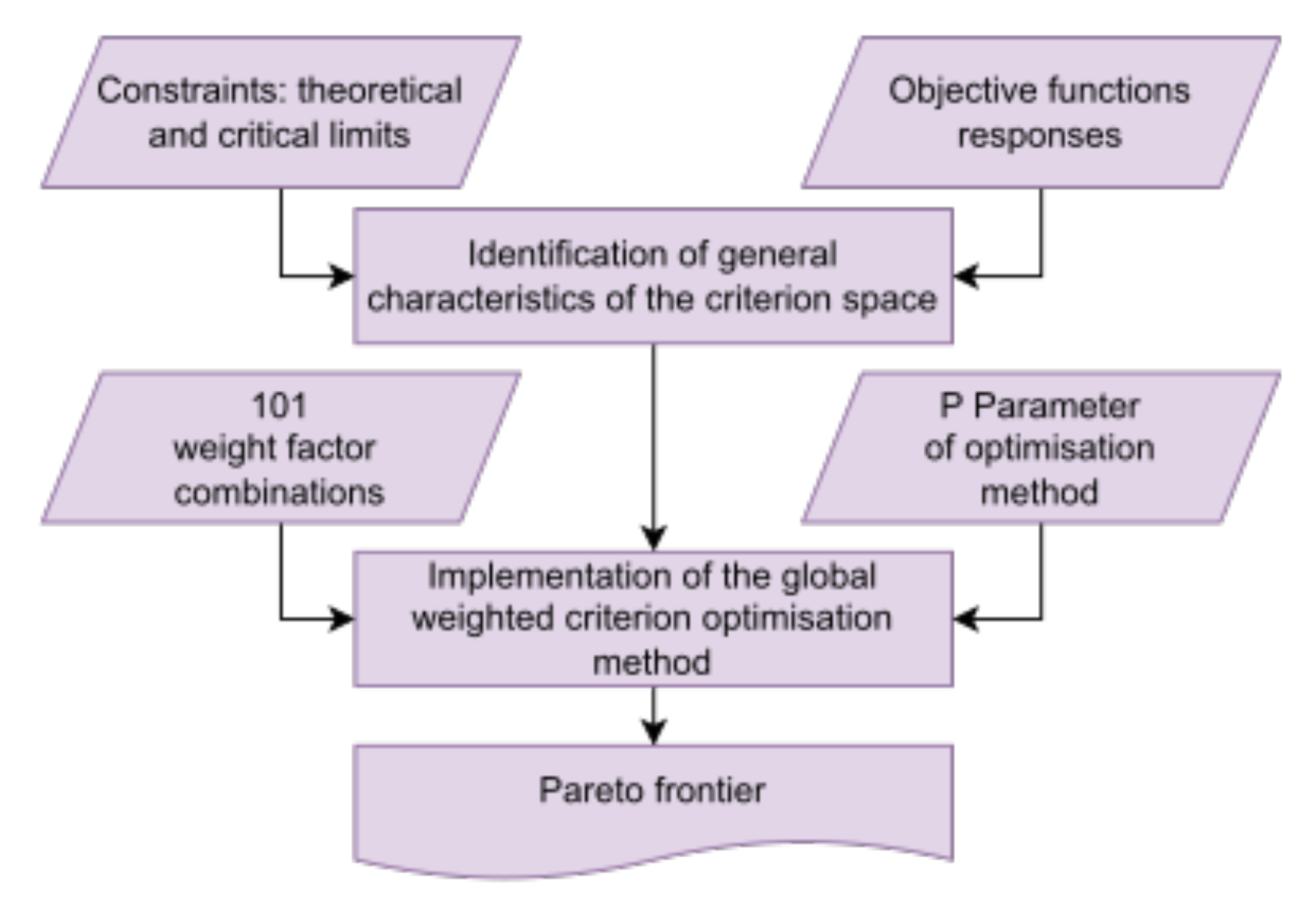
The optimisation process is the final stage of the methodology. It involves constructing surrogate models to link S and L with $Cl$ and $f_f$ to predict the behaviour of unsampled data points, and a code that solves Equations (5) and (13) for different $\xi$, to describe the structural dynamics of the device. Figure 13 illustrates the methodology developed in this sub-stage, which includes the phases of constructing the criterion space and implementing the optimisation method, along with their inputs and outputs. The subsequent subsection delves deeper into the description of the weighted global criterion method, which allows for defining the Pareto frontier.

The Weighted Global Criterion Method

The weighted global criterion method is a transformation option that combines multiple objective functions in a singular format for general minimisation.

Equation (18) presents the most common weighted global criterion [39]. In this equation, U is the minimisation function, $f_i\left(x\right)$ is an independent objective function evaluated on x, $f_i^o$ is the utopic value of the objective function, $w_i$ is a weight factor of an objective function, and p is a parameter of the model that measures the relevance of minimising the U function with the highest difference between $f_i\left(x\right)$ and $f_i^o$. Therefore, large values of p (theoretically infinite) allow identifying points on the Pareto frontier for each combination of weights, whether this frontier presents a convex or non-convex curvature.

$$U={\left\{\sum _{i=1}^k{\left[w_i\left(f_i\left(x\right)-{f_i}^o\right)\right]}^p\right\}}^{\frac{1}{p}}$$

(18)

Objective functions can exhibit different orders of magnitude, which leads to numerical errors due to the nature of computers. Equation (19), however, enables the reduction of such errors by scaling the objective functions, as suggested by Arora [39]. This equation incorporates the utopian value $\left(f_i^o\right)$ and the maximum value attained by the objective function under study $\left(f_i^{max}\right)$, both of which are necessary for obtaining a scale of normalised values.

$$U={\left\{\sum _{i=1}^k{\left[w_i\left(\frac{f_i\left(x\right)-{f_i}^o}{{f_i}^{max}-{f_i}^o}\right)\right]}^p\right\}}^{\frac{1}{p}}$$

(19)

Finally, Equation (20) allows computing the utopian values $f_i^o$, where ${\left(f_i^o\right)}^{\prime }$ represents a restrictive condition of the apparatus, ${\left(f_i\right)}_{min}$ the minimum value of the objective function in generated data, and $\alpha$ is a user-setting parameter that depends on the level of performance required in the design. Given that the utopian values are always lower than the minimum observations of the design objective, this parameter has to be lower than one [31].

$${f_i}^o={\left({f_i}^o\right)}^{\prime }+\alpha \left[{\left(f_i\right)}_{min}-{\left(f_i^o\right)}^{\prime }\right]$$

(20)

4. Results Analysis

4.1. Mesh Sensitivity Analysis

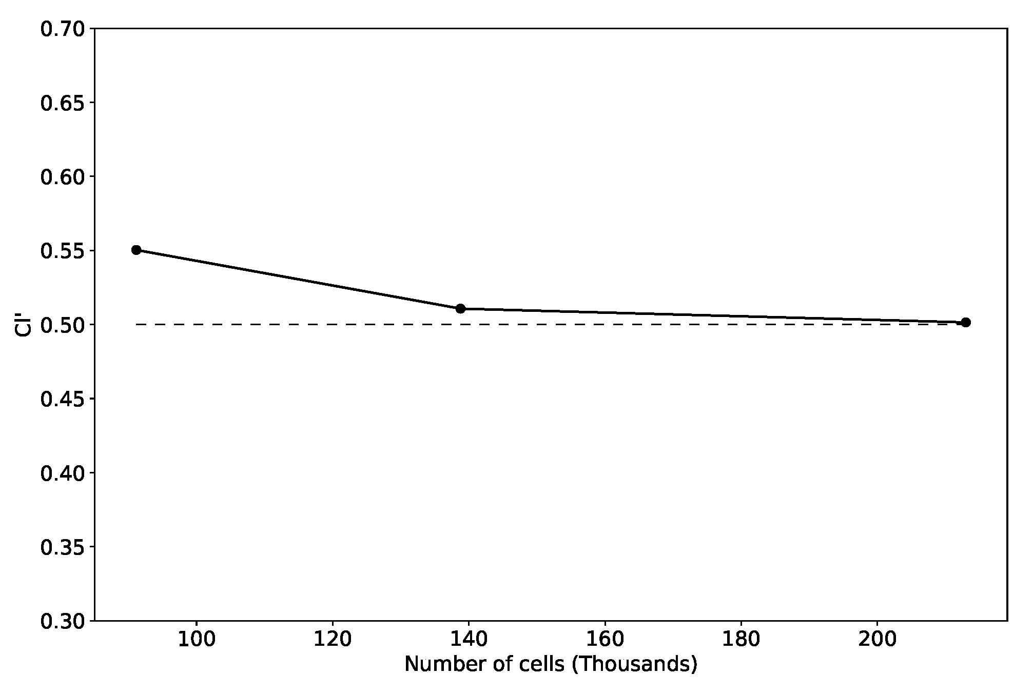
The domain discretisation started with 91,155 cells, according to Section 3.2.3, and incremented its resolution with a factor of 1.5 on each test during the sensitivity analysis (see

Table 4. Mesh configuration during the validation.

Case	Divisions	Number of cells
M1	74	91,155
M2	116	138,765
M3	181	212,985

). Meanwhile, discrepancies between the Lift Coefficient and the Strouhal number computed by CFD and reported by Norberg [17] allowed for assessing their performance.

Figure 14 displays a graphical representation of the lift coefficient ($C{l}^{\prime }$) predicted from CFD using the discretisation detailed in Table 4.

Table 5. CFD results comparison using [17] as the benchmark.

Case	Cl	St	Error Cl (%)	Error St (%)
Experimental	0.500	0.198	-	-
M1	0.550	0.208	10.067	5.422
M2	0.511	0.192	2.142	2.816
M3	0.501	0.197	0.285	0.238

, on the other hand, presents the CFD results for the lift coefficient, Strouhal number, and computed error between CFD and experimental data [17]. The CFD simulations always overestimate the RMS lift coefficient, while the Strouhal number exhibits oscillatory behaviour. Among all the cases, Case M3 produces the most accurate results with a percentage error of less than 1% for both the lift coefficient and the Strouhal number. Based on these results, Case M3 serves as the baseline discretisation during the optimisation.

Figure 15 illustrates the Kolmogorov energy spectrum computed from the instantaneous velocity field measured by two probes located downstream from the cylinder at distances of 1D and 1.5D, using the mesh resolution from Case M3. The graph also shows a dashed line with a slope of $\frac{-5}{3}$ to represent the typical energy spectrum trend at the inertial scale. A simple comparison of the trends confirms that the LES filter is small enough within the studied region.

4.2. Aerodynamic Behaviour of the Cylinder-Plate Configuration

The aerodynamic study of the cylinder-plate configuration implemented a DOE according to Section 3.2.4. Figure 16 shows the sampling location, where S and L represent the cylinder-plate separation and plate length (see Figure 11).

Figure 17 shows an example of the mesh used in the CFD evaluation. The number of inflation layers near the plate is 22, with a growth rate of 1.15. The cases studied maintain a mesh resolution equal to Case M3 in the vicinity of the cylinder to ensure accurate prediction of vortex shedding.

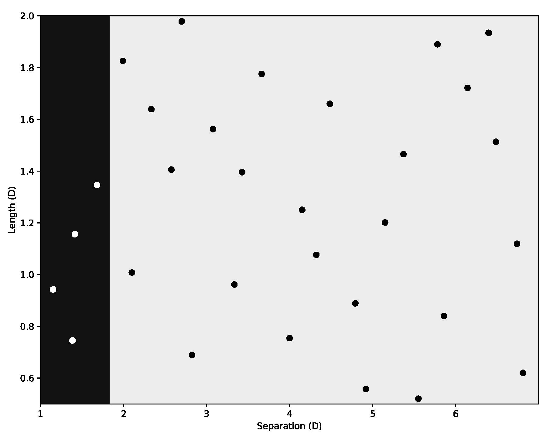
Figure 18 shows an instantaneous value of the fluid vorticity for two selected cases from the evaluated sampling. Case (a) represents a scenario where S/D = 2.099, L/D =1.008 and vortex shedding occurs. Case (b), moreover, represents a scenario where S/D = 1.258, L/D = 1.979 and vortex suppression appears due to the plate’s proximity to the cylinder. The classification method described in Section 3.2.6, with a decision boundary of $C{l}^{\prime }\ge 0.45$, allows for discarding the suppression condition.

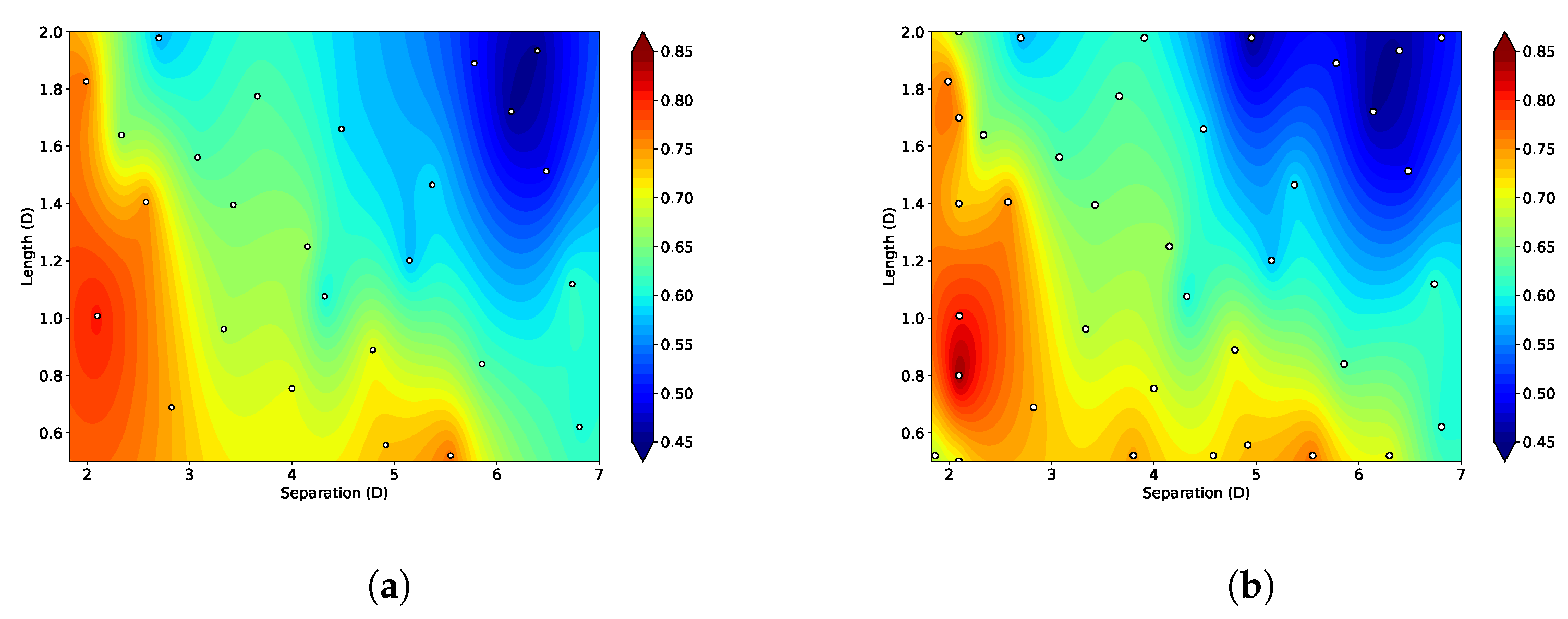
Figure 19 presents the outcomes from the classification method. The black region represents the design space where the vortex shedding suppression occurs (S/D $\le 1.83$). Eliminating the vortex shedding suppression region modifies the evaluation range of cylinder-plate separation to 1.83 ≥ S/D ≥ 7 and reduces the number of samples to 26 (13 per variable). With this smaller dataset, a Kriging model to predict $C{l}^{\prime }$ allowed an NRMSE of $15.5\%$ during the implementation of the lift-one-out technique. However, 12 new samples placed on regions of high error, detected during the surrogate model validation process, allowed for maintaining the original sample size and a final reduction of the NRMSE to $12.42\%$.

Figure 20 displays the contour plots of $C{l}^{\prime }$ before and after the implementation of the sampling enhancement. The new samples do not significantly alter the overall patterns within the design space; however, they improve the localised resolution of specific areas, resulting in a more accurate estimation of the maximum and minimum values of $C{l}^{\prime }$. This improvement allows for a better prediction of the optimal Power Coefficient.

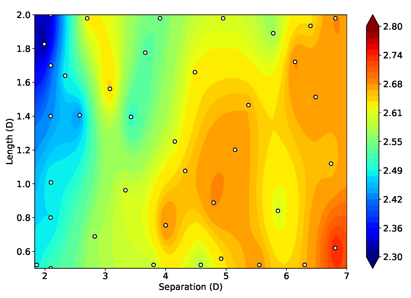
Regarding the vortex shedding frequency, Figure 21 shows its contour plot using the resulting 38 samples from the mentioned validation process. The Kriging model is capable of predicting values for this variable with an NRMSE of $13.08\%$.

4.3. Structural Behaviour of the Cylinder-Plate Configuration

The following results come from the procedures outlined in Section 3.3. The objective is to determine a potential increase in the device’s power coefficient $\left(F_1\right)$ and a decrease in its displacement $\left(F_2\right)$ while varying the damping factor value between 0.01 and 0.05. Nevertheless, good optimisation practices aim to define objective functions that require minimisation. Therefore, this study replaces an increment of the device power coefficient $\left(C_p\right)$ with a reduction of the unused energy ratio $(1-C_p)$.

Figure 22 depicts the response of the oscillating system according to Newton’s Second Law of Motion for different values of the damping factor, plate length, and cylinder separation. The dashed lines in the figure indicate the limiting conditions of the machine; ${F_1^0}^{\prime }$ is 0.41, which corresponds to the minimum ratio of unused energy according to the momentum theory—Betz law [40], while ${F_2^0}^{\prime }$ is zero, corresponding to the minimum displacement condition of the system achieved at a high damping coefficient. The grey frame, on the other hand, defines the criterion space based on the ideal $\left({F_i}^0\right)$ and critical $\left(F_i^C\right)$ values of the objective functions. The utopic values come from Equation (20) when $\alpha$ is 0.9, while the critical values are 0.5D for the lateral displacement and 1 for the ratio of unused energy, indicating the absence of power production.

Figure 23 displays the normalised values of the perpendicular displacement and the ratio of unused energy obtained from the data within the grey box of Figure 22; the normalisation considers the machine’s restrictive conditions (${F_i^0}^{\prime }$) and critical values ($F_i^C$). Equation (19) allows for the computation of the Pareto frontier of this figure using a value of p equal to 145, which is high enough to perform the optimisation while avoiding any relevant computer round-off errors. The weighting factor changes from 0–1 with a step size of 0.1, while the colours in the Pareto frontier represent the variables S, L, and $\xi$, respectively.

Figure 23 indicates that a cylinder plate separation between $0.7$ and $0.8$ represents an extensive part of the Pareto frontier. However, large values of this variable give a high-power coefficient and a high perpendicular displacement of the device. Conversely, a lower value for this variable leads to the opposite effect. Furthermore, the plate length shows consistent variations throughout the Pareto frontier, with values mainly ranging between $0.45$ and 0. Finally, most points on the Pareto frontier report low values of $\xi$. However, high values of this variable significantly reduce the perpendicular displacement of the device.

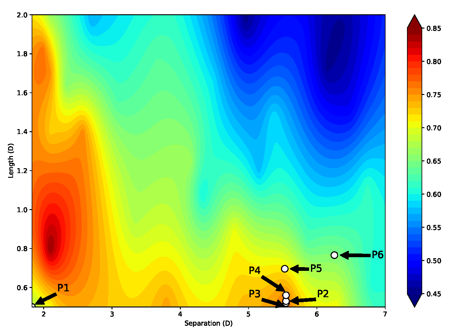
The Euclidean distance calculation between the computed and the utopian condition allows for determining the scenario that provides the ideal outcome based on the weighting factors.

Table 6. Single and multi-objective optimum points.

Case	Weight $({\mathit{F}}_1-{\mathit{F}}_2)$	Euclidian Distance	F1 Value (Normalised)	F2 Value (Normalised)	$\mathit{\xi }$	S/D Value	L/D Value
P1	0.00–1.00	0.987	0.996 (0.987)	0.008D (0.016)	0.050	1.830	0.500
P2	0.25–0.75	0.778	0.921 (0.739)	0.122D (0.244)	0.024	5.548	0.530
P3	0.47–0.53	0.683	0.853 (0.513)	0.226D (0.451)	0.013	5.548	0.520
P4	0.50–0.50	0.688	0.845 (0.488)	0.242D (0.485)	0.013	5.548	0.560
P5	0.75–0.25	0.800	0.774 (0.252)	0.380D (0.759)	0.010	5.530	0.696
P6	0.90–0.10	0.998	0.731 (0.109)	0.496D (0.992)	0.010	6.343	0.766

shows six optimum configurations (Cases P1–P6) as follows. The first and the last row presents the optimum condition after considering the perpendicular displacement or the ratio of unused energy alone. The other rows represent the multi-objective optimal scenarios, where the third row exhibits the minimum Euclidean distance calculated from all of the evaluated conditions.

The distance between the pole and the plate remains almost constant in P2, P3, and P4 cases. However, as the length increases, $F_1$ decreases while $F_2$ increases. On the other hand, the damping coefficient produces the opposite effect. Case P6 gives the maximum power coefficient, with a value of $0.269$$(1-F_1)$, but it also offers the maximum displacement of 0.496D.

By selecting Case P3 as the optimal choice, the desired configuration requires a plate with a length of 0.52D, a separation of 5.548D from the cylinder, and a damping factor of $0.013$. This design results in a perpendicular displacement of 0.226D (normalised: 0.451D) and a ratio of unused energy of $0.853$ (normalised: $0.513$). This configuration can achieve a power coefficient of 13.07% and 196% higher than the single blade-less turbines Vortex Nano and Vortex Tacoma, respectively, under similar wind speeds.

Figure 24 illustrates the configurations presented in Table 6 and the $C{l}^{\prime }$ contour. It is worth noting that there is a significant disparity between condition one and the others; this may be due to the prioritisation of displacement reduction in condition one without considering the energy generated. In contrast, the remaining cases are in a region where the lift coefficient varies from moderate to high, particularly in Cases P2, P3, and P4. These findings indicate that the lift coefficient plays a critical role in the optimisation process of these generators, especially when the design aims to achieve high power coefficients followed by the device size reduction.

5. Conclusions

The following conclusions derive after reviewing the results of this study:

• The Kriging surrogate model integrated with a classification method allowed identifying a zone within the sampling space where the vortex suppression occurs. To prevent this effect, a gap between the plate and the cylinder must be higher than $1.83\left(\frac{\mathrm{S}}{\mathrm{D}}\right)$ for similar configurations and conditions.
• Results from the multi-objective optimisation showed that, under the given constraints, this type of wind generator produces a power coefficient of up to $0.269$ when its oscillation amplitude is at its maximum (0.5D). Moreover, from all the evaluated configurations, a design with $\xi =0.013$, $\frac{\mathrm{S}}{\mathrm{D}}=5.548$ and $\frac{\mathrm{L}}{\mathrm{D}}=0.520$ provides the closest match to the utopian condition.
• Finally, the results obtained in this study suggest that the configuration with the minimum Euclidean distance to the Pareto frontier offers an increase of $13.07\%$ in the value of the power coefficient concerning the Vortex Nano blade-less generator in similarly windy conditions.

References

1. Sumathi, S.; Kumar, L.; Surekha, P. Solar PV and Wind Energy Conversion Systems: An Introduction to Theory, Modeling with MATLAB/SIMULINK, and the Role of Soft Computing Techniques; Green Energy and Technology; Springer International Publishing: Berlin/Heidelberg, Germany, 2015. [Google Scholar]
2. Hau, E.; Renouard, H. Wind Turbines: Fundamentals, Technologies, Application, Economics; Springer: Berlin/Heidelberg, Germany, 2013. [Google Scholar]
3. Yáñez Villarreal, D.J. VIV Resonant Wind Generators—Vortex Bladeless Wind Power. 2018. Available online: https://vortexbladeless.com/wp-content/uploads/2018/10/VortexGreenPaper_en.pdf (accessed on 2 February 2023).
4. Cajas García, J.C.; Houzeaux, G.; Yáñez, D.J.; Mier-Torrecilla, M. SHAPE Project Vortex Bladeless: Parallel Multi-Code Coupling for Fluid-Structure Interaction in Wind Energy Generation; Partnership for Advanced Computing in Europe: Brussels, Belgium, 2016. [Google Scholar]
5. Francis, S.; Umesh, V.; Shivakumar, S. Design and Analysis of Vortex Bladeless Wind Turbine. Mater. Today Proc. 2021, 47, 5584–5588. [Google Scholar] [CrossRef]
6. Mane, A.; Kharade, M.; Sonkambale, P.; Tapase, S.; Kudte, S.S. Design & analysis of vortex bladeless turbine with gyro e-generator. Int. J. Innov. Res. Sci. Eng. 2017, 3, 445–452. [Google Scholar]
7. Chizfahm, A.; Yazdi, E.A.; Eghtesad, M. Dynamic modeling of vortex induced vibration wind turbines. Renew. Energy 2018, 121, 632–643. [Google Scholar] [CrossRef]
8. Shahat, A.E.; Hasan, M.; Wu, Y. Vortex Bladeless Wind Generator for Nano-Grids. In Proceedings of the 2018 IEEE Global Humanitarian Technology Conference (GHTC), San Jose, CA, USA, 18–21 October 2018; pp. 1–2. [Google Scholar]
9. Tandel, R.; Shah, S.; Tripathi, S. A state-of-art review on Bladeless Wind Turbine. J. Phys. Conf. Ser. 2021, 1950, 012058. [Google Scholar] [CrossRef]
10. Aballe, A.B.D.; Cruz, K.Y.C.; Rosa, V.J.H.D.; Magwili, G.V.; Ostia, C.F. Development of a Linear Generator With Spring Mechanism for Vortex Bladeless Wind Turbine. In Proceedings of the 2020 IEEE 12th International Conference on Humanoid, Nanotechnology, Information Technology, Communication and Control, Environment, and Management (HNICEM), Manila, Philippines, 3–7 December 2020; pp. 1–6. [Google Scholar] [CrossRef]
11. Ordoñez, O.; Duke, A.R. Wind Resource Assessment: Analysis of the Vortex Bladeless Characteristics in Puerto Cortés, Honduras. Iop Conf. Ser. Earth Environ. Sci. 2021, 801, 012019. [Google Scholar] [CrossRef]
12. Eldredge, J.D.; Pisani, D. Passive locomotion of a simple articulated fish-like system in the wake of an obstacle. J. Fluid Mech. 2008, 607, 279–288. [Google Scholar] [CrossRef] [Green Version]
13. Wu, J.; Shu, C. Numerical study of flow characteristics behind a stationary circular cylinder with a flapping plate. Phys. Fluids 2011, 23, 073601. [Google Scholar] [CrossRef]
14. Wang, H.; Zhai, Q.; Zhang, J. Numerical study of flow-induced vibration of a flexible plate behind a circular cylinder. Ocean Eng. 2018, 163, 419–430. [Google Scholar] [CrossRef]
15. Eydi, F.; Mojra, A.; Abdi, R. Comparative analysis of the flow control over a circular cylinder with detached flexible and rigid splitter plates. Phys. Fluids 2022, 34, 113604. [Google Scholar] [CrossRef]
16. Lee, C.M.; Paik, K.J.; Kim, E.S.; Lee, I. A fluid–structure interaction simulation on the wake-induced vibration of tandem cylinders with pivoted rotational motion. Phys. Fluids 2021, 33, 045107. [Google Scholar] [CrossRef]
17. Norberg, C. Fluctuating lift on a circular cylinder: Review and new measurements. J. Fluids Struct. 2003, 17, 57–96. [Google Scholar] [CrossRef]
18. White, G. Introduction to Machine Vibration; Reliabilityweb.com: Fort Myers, FL, USA, 2008. [Google Scholar]
19. The-SciPy-Community. Fourier Transforms (Scipy.fft). 2023. Available online: https://docs.scipy.org/doc/scipy/tutorial/fft.html (accessed on 28 February 2023).
20. Rao, K.R.; Yip, P. The Transform and Data Compression Handbook; CRC Press, Inc.: Boca Raton, FL, USA, 2000. [Google Scholar]
21. Cengel, Y.A.; Cimbala, J.M. Mecánica De Fluidos 4a Edición; Mcgraw Hill: New York, NY, USA, 2018. [Google Scholar]
22. Damiána, S.M.; Nigro, N.M. Comparison of single phase laminar and Large Eddy Simulation (LES) solvers using the Openfoam R suite. Mecánica Comput. 2010, 29, 3721–3740. [Google Scholar]
23. Blazek, J. Computational Fluid Dynamics: Principles and Applications; Elsevier Science: Amsterdam, The Netherlands, 2015. [Google Scholar]
24. OpenCFD-Ltd. OpenFOAM User Guide: Smagorinsky. Available online: https://www.openfoam.com/documentation/guides/latest/doc/guide-turbulence-les-smagorinsky.html (accessed on 17 November 2022).
25. Berselli, L.; Iliescu, T.; Layton, W. Mathematics of Large Eddy Simulation of Turbulent Flows; Scientific Computation; Springer: Berlin/Heidelberg, Germany, 2006. [Google Scholar]
26. Sagaut, P.; Meneveau, C. Large Eddy Simulation for Incompressible Flows: An Introduction; Scientific Computation; Springer: Berlin/Heidelberg, Germany, 2006. [Google Scholar]
27. SimScale. Large Eddy Simulation—Flow over a Cylinder. Available online: https://www.simscale.com/docs/validation-cases/large-eddy-simulation-flow-over-a-cylinder/ (accessed on 8 March 2023).
28. ANSYS, I. ANSYS FLUENT 12 User’s Guide; ANSYS Inc.: Canonsburg, PA, USA, 2009. [Google Scholar]
29. White, F.M. Fluid Mechanics, 7th ed.; Mcgraw-Hill Series in Mechanical Engineering; McGraw-Hill: New York, NY, USA, 2011. [Google Scholar]
30. Cao, Y.; Tamura, T. Numerical investigations into effects of three-dimensional wake patterns on unsteady aerodynamic characteristics of a circular cylinder at Re=1.3×10⁵. J. Fluids Struct. 2015, 59, 351–369. [Google Scholar] [CrossRef]
31. Spanelis, A.; Walker, A.D. A Multi-Objective Factorial Design Methodology for Aerodynamic Off-Takes and Ducts. Aerospace 2022, 9, 130. [Google Scholar] [CrossRef]
32. Kleijnen, J.P. Design and Analysis of Simulation Experiments; International Series in Operations Research & Management Science; Springer: Berlin/Heidelberg, Germany, 2015. [Google Scholar]
33. Chen, V.C.; Tsui, K.L.; Barton, R.R.; Meckesheimer, M. A review on design, modeling and applications of computer experiments. IIE Trans. 2006, 38, 273–291. [Google Scholar] [CrossRef]
34. Simpson, T.W.; Poplinski, J.D.; Koch, P.N.; Allen, J.K. Metamodels for Computer-based Engineering Design: Survey and recommendations. Eng. Comput. 2001, 17, 129–150. [Google Scholar] [CrossRef] [Green Version]
35. Murphy, B.; Yurchak, R.; Müller, S. GeoStat-Framework/PyKrige: v1.7.0. 2022. Available online: https://geostat-framework.readthedocs.io/_/downloads/pykrige/en/latest/pdf/ (accessed on 3 March 2023).
36. Akilli, H.; Sahin, B.; Filiz Tumen, N. Suppression of vortex shedding of circular cylinder in shallow water by a splitter plate. Flow Meas. Instrum. 2005, 16, 211–219. [Google Scholar] [CrossRef]
37. Dai, S.; Younis, B.A.; Zhang, H.; Guo, C. Prediction of vortex shedding suppression from circular cylinders at high Reynolds number using base splitter plates. J. Wind Eng. Ind. Aerodyn. 2018, 182, 115–127. [Google Scholar] [CrossRef] [Green Version]
38. Shabana, A. Theory of Vibration: An Introduction; Mechanical Engineering Series; Springer International Publishing: Berlin/Heidelberg, Germany, 2019. [Google Scholar]
39. Arora, J.S. (Ed.) Introduction to Optimum Design, 3rd ed.; Academic Press: Boston, MA, USA, 2011. [Google Scholar]
40. Sons, J.W. (Ed.) The Wind Resource. In Wind Energy Handbook; John Wiley & Sons, Ltd.: Hoboken, NJ, USA, 2011; Chapter 2; pp. 9–38. [Google Scholar] [CrossRef]
Figure 1. Power coefficients of different wind turbines [2].
Resources 12 00090 g001
Figure 2. Scheme of bladeless generators.
Resources 12 00090 g002
Figure 3. CAD model of the proposed concept of wind generator.
Resources 12 00090 g003
Figure 4. Domain configuration to assess the optimisation process.
Resources 12 00090 g004
Figure 5. Graphic representation of perpendicular displacement.
Resources 12 00090 g005
Figure 6. Diagram of Surrogate Model Stage.
Resources 12 00090 g006
Figure 7. Domain configuration for the validation of the CFD model (free stream that crosses a cylinder).
Resources 12 00090 g007
Figure 8. Mesh with 181 divisions along the cylinder circumference.
Resources 12 00090 g008
Figure 9. Isometric view of the mesh.
Resources 12 00090 g009
Figure 10. LHS of two variables with five intervals, where each dot represents a sample [33].
Resources 12 00090 g010
Figure 11. Domain configuration to assess the effect of the Von Kármán Vortex Street on aerodynamic shapes.
Resources 12 00090 g011
Figure 12. Diagram of Structural Dynamics Modelling Stage.
Resources 12 00090 g012
Figure 13. Diagram of optimisation process methodology.
Resources 12 00090 g013
Figure 14. CFD trend on the C l prediction during the mesh refinement; the dashed line represents the target value of C l .
Resources 12 00090 g014
Figure 15. Kolmogorov energy spectrum post-processed from the instantaneous velocity field of Case M3 at (a) 1D and (b) 1.5D downstream from the cylinder (wake zone).
Resources 12 00090 g015
Figure 16. Latin hypercube sampling.
Resources 12 00090 g016
Figure 17. Domain discretisation of a sample from the studied sampling.
Resources 12 00090 g017
Figure 18. Vorticity contour for samples (a) without and (b) with vortex suppression. Parameters used for these simulations are disclosed in Table 1, Table 2 and Table 3.
Resources 12 00090 g018
Figure 19. Decision tree classification of the sampling—decision boundary at 0.45 for the Cl′ (black region reports the vortex shedding suppression).
Resources 12 00090 g019
Figure 20. Contour of Lift Coefficient C l —(a) Kriging function built from 26 samples and (b) Kriging function built from 38 samples.
Resources 12 00090 g020
Figure 21. Contour of f f —Kriging function built from 38 samples.
Resources 12 00090 g021
Figure 22. Response of the Oscillatory System to Sampling: Analysis of Damping Factors (0.01, 0.0275 and 0.05) and Spatial Criteria.
Resources 12 00090 g022
Figure 23. Pareto frontier—the colour map indicates values of (a) S, (b) L, (c) ξ along the frontier.
Resources 12 00090 g023
Figure 24. Lift coefficient contour (Cl) built from 38 samples and optimum configurations (P1–P6) from Table 6.
Resources 12 00090 g024