Contribution of Landscape Transformation in the Development of Heat Islands and Sinks in Urban and Peri-Urban Regions in the Chota–Nagpur Plateau, India

Abstract

Cities in the contemporary world are experiencing shifts in local climatic conditions that are primarily linked to rapid urban growth, carbon emissions, and environmental degradation. In the present study, land surface temperature (LST) in urban and peri-urban regions of the city of Ranchi was estimated and correlated with land use/land cover (LULC) using temporal LANDSAT satellite images from 2000 to 2014 on a bi-annual basis. The study exhibited a gradual increase in built-up land with total growth of 47.65 sq. km (135%) at the cost of vegetation (−6.8%), rock outcrops (−44.16%), and other LULCs (0.81%). Spatiotemporal LST variability exhibited an increase in area under high-temperature (>38 °C) zones as compared to moderate (30 °C to 38 °C) and low-temperature (<30 °C) zones. Although the LST distinctively escalated in all LULC in the month of May from 2000 to 2014, urban areas exhibited cooler conditions than their environs at a regional scale, except for 2006. A higher surface temperature was observed over bare rock (min/max: 28–43 °C), fallow land (25–42 °C), and industrial built-up areas (31–43 °C), followed by vegetation (24–34 °C) and waterbodies (22–30 °C). The rapid land transformation to an impervious surface, degradation of vegetation coverage and its health, deforestation due to urbanization, the dumping of non-treated wastewater into reservoirs, and pollution altogether led to an increase in urban heat islands (UHI). The study demonstrated that the LST increased in urban regions but appeared cooler than those of its peri-urban counterparts because of the presence of barren land and rock outcrops. The existing tenancy act had an indirect impact on maintaining natural landscapes and controlling the LST within the Ranchi region. The study recommends nature-based solutions in terms of plantation and green roofing within the rising LST zones located in the urban core and in peripheral rock outcrops collectively to minimize the rising impact of LST in urban and peri-urban regions.

1. Introduction

The characteristics of the urban climate are determined by geographical location and the local climate of cities, in addition to human activity and the built environment. It is a well-known fact that urban design parameters and practices highly influence the urban microclimate. Rapid unplanned urban growth has transformed cities into clusters of asphalt, concrete, brick, and impervious surfaces [1], replacing natural forests [2] and agricultural land [3]. This frequently leads to a decrease in soil moisture and evapotranspiration [4,5,6] and releases significant amounts of waste heat into the urban atmosphere, which can disrupt the appearance of micro and mesoscale climates [7,8]. The increase in temperature due to this rural–urban transformation helps to quantify the changes in energy balance and improve and develop spatial planning in the consideration of different mitigation measures such as urban greening, rooftop gardening, green walls, green corridors, etc. [9,10] The population residing in urban areas has increased from 30% in 1950 to 55% in 2018. By 2045, the number of people living in cities will have increased by 1.5 times to 6 billion, adding 2 billion more urban residents [11]. Anthropogenic heat flux by vehicles, industries, and complex urban structures directly affects microclimatic variables such as mean radiative temperature, humidity, and air quality, contributing to the urban heat island (UHI) phenomenon [12]. Surface materials such as pavements and building roofs strongly influence the urban local climate, based on their ability to absorb, reflect, and transmit solar radiation [13], which depends on the color of paving or building materials [14].

UHI is a global phenomenon of specifically urban climates [15,16] that differs from surrounding rural areas due to a prominent modification of air and near-surface temperatures in which urban areas experience higher temperatures than surrounding non-urban areas [17,18]. Several environmental changes are caused by the UHI, including vegetation growth [19] regional climate [20,21] and water and air quality [22]. The amount of solar radiation that is absorbed, reflected, and received by an urban area depends on aerosol content, cloud cover, and surface characteristics such as topography and land use [23]. Urban areas absorb more solar radiation, have greater thermal conductivity, and are better able to release daytime heat at night [24]. The impervious nature of urban surface material hampers the infiltration rate, resulting in a decrease in soil moisture and evapotranspiration as a consequence of urban forests and green-space degradation [25]. Aerodynamic surface structure and radiation fluxes have a significant impact on the local energy budget and modify the local climate [26,27,28]. A major indicator of a UHI is the spatial distribution of land surface temperature (LST), which is controlled by surface heat fluxes, a dynamic phenomenon that changes over time in both intensity and spatial distribution [29]. UHI has a direct impact on the environment, energy use, economy, mortality rates, human health and comfort, and regional climates [30,31] and increases the energy demands with a yearly increase of 7% CO₂ emission in summer [32]. In particular, UHI influences higher temperatures, wind patterns, precipitation rates, and cycles, and amplifies heat waves, additional showers, and thunderstorms with fog and clouds [33,34]. Even though a large pool of research has been carried out with respect to the quantification of UHI, the cause and implication of UHI must be thoroughly investigated to meet upcoming challenges [35].

It is well established that geoinformatics is used to study urban growth processes and LST, and, more specifically, the relationship between spatiotemporal land-use transformations (LUT) and LST dynamics [36,37]. Remote-sensing data are valuable sources of information because they can be integrated with geographic information systems [38,39] with multispectral, spatial, and temporal capabilities that can be used to obtain current data over large areas at a low cost [40]. Earth observation-based LST offers efficient measurements that help monitor climate modifications, microclimates, and climate variabilities continuously at different spatiotemporal scales [41]. The exploitation of satellite data in surface urban heat island intensity (SUHI) estimation helps to monitor urban–rural LST variations contributed by imperviousness, landscape structure, and climate of the region [42]. There are several methods for the estimation of land surface temperatures, such as the Radiative Transfer Equation (RTE) method, the Mono Window Algorithm (MWA), and the Split Window Algorithm (SWA) using Landsat data series [43]

UHI studies using ground-based air temperature measurements are accurate and reliable, but they do not adequately represent the large area. An alternative and trustworthy method for estimating spatiotemporal LST for large areas and its relationship with LUT is thermal remote sensing [44]. The biophysical characteristics of the land surface and estimation of LST are typically observed and modeled using LANDSAT Thematic Mapper (TM), Enhanced Thematic Mapper Plus (ETM⁺), and LANDSAT 8 Thermal Infrared Sensor (TIRS) images [45]. Some studies have used pixel-by-pixel statistical correlation analysis between surface temperature, vegetation indices, and porosity to estimate UHI [15], while others have used a linear regression between LST and NDVI [46,47]. The main factors that contribute to the formation of an urban heat sink (UHS) are attributed to the time of image acquisition, the state of rural bare soil, the state of rural dry soil, low rural surface thermal inertia, and other factors that were identified by analyzing LANDSAT TM thermal data and atmospheric temperature data [7,48]. On the other hand, because dry soils have lower thermal capacities and conductivities than wet soils, they also play a role in the reduction of rural surface thermal inertia. The warming trend has been reported in many Indian cities, notably Delhi [49], Noida [50], Pune [51], and Chennai [52].

With increasing research on the cause and effects of UHI on human health and the environment, a detailed investigation is much needed to understand the long-term influence of landscape transformation on the development of UHI and alteration in cool islands and heatsink zones to frame a suitable urban policy, especially for future growth regulations and sustainable landscape management practices. Even though Ranchi had very pleasant weather conditions until recently and was the summer capital of Madagh during the British era, a significant change in the local climate [53], deterioration in the urban environmental conditions [54,55], and groundwater quality [40,56] have become prevalent due to high population influx induced rapid built-up land growth and significant land-use transformation. Previous studies have reported a rapid and haphazard urban sprawl in Ranchi largely contributing to increasing LST (34–42 °C) as compared to the rural environment (30–38 °C) based on the meteorological tower statistics [53]. Therefore, in the present study, an attempt has been made to assess the spatiotemporal variability in LST in Ranchi’s urban and peri-urban regions from 2000 to 2014 to deduce the relationship between LST and LULC in a dynamic mode after the reorganization of Ranchi as the state capital on a bi-annual basis. Furthermore, the study elucidates the importance of potential heat sink zones and their interrelationship with UHI in urban and peri-urban regions.

Study Area

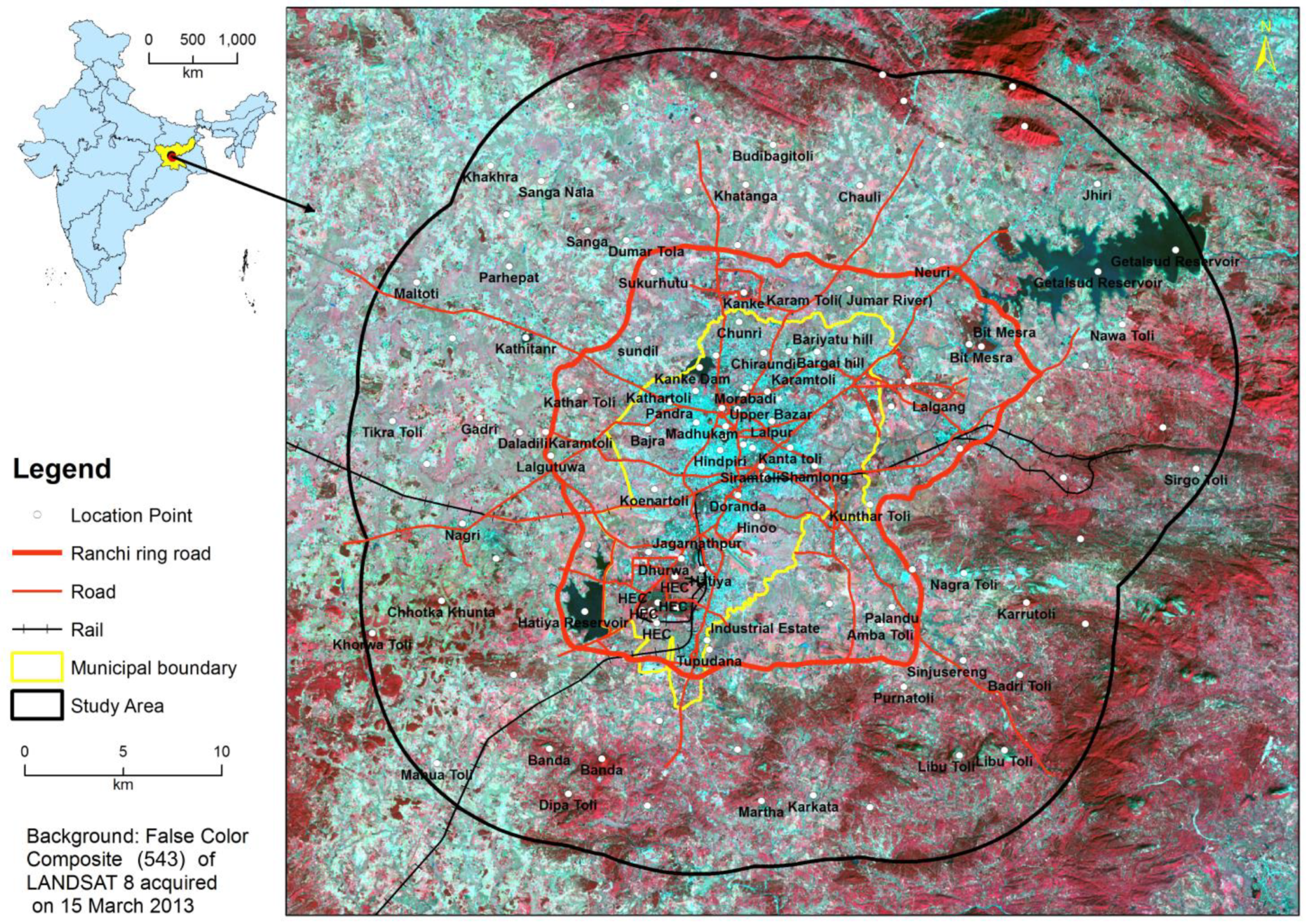
The present study was conducted in Ranchi urban and peri-urban regions, which have an area of 1516.72 sq. km. and are situated on the Chota–Nagpur plateau, which is in the northeastern part of the peninsular of India. It is located between 85°07′ and 85°34′ E longitude and 23°11′ to 23°32′ N latitude with an average elevation of 640 m above sea level. The demarcation of the study area was made using the 10 km outer buffer of the newly constructed Ranchi Ring Road, which covers primarily all urban dwellings and mainly consists of settlements in Ranchi conurbation, its fringe area, and neighboring rural areas. The study area incorporates the Ranchi Municipal Corporation (RMC) area of about 173 sq. km (Figure 1) and mainly covers a major part of the Kanke, Namkum, and Ratu community development blocks. The built-up land expands beyond the municipal limits, as evident on NH-33 and NH-75, with high-end medical facilities, educational institutions, housing, and roadside commercial activities. Due to its regional importance, it acts as a centripetal force and limits the growth of other urban centers in its hinterland [55].

The population of the Ranchi Urban Area rapidly increased from 599,000 to 844,000 people from 1991 to 2001, and increased to 1,137,000 people in 2011. The high rate of population growth has grown the city’s surface structure haphazardly and in an unplanned manner, which has had a negative impact on the environment of Ranchi [54,55]. The state falls under the tropical monsoon climatic region. The Tropic of Cancer passes through the middle of Ranchi. It has an average summer temperature range of 24 °C to 37.2 °C and an average winter temperature range of 10.3 °C to 22.9 °C. The average monsoon rainfall received from June to October is 1000 mm, while the average annual rainfall is 1260 mm. This area has three main seasons: winter, which extends from October to February; summer, which extends from March to May; and the rainy season, which extends from June to September. The mean annual humidity is 62%, and the average velocity of the wind is 6.6 km h⁻¹. The intensity and pattern of rainfall are conspicuous, erratic, and changing every year. Although rainfall in Ranchi begins in the month of June, reaches its maximum intensity in July–August, and ends in October, there could also be rainfall during the winter season.

2. Data Used and Methodology

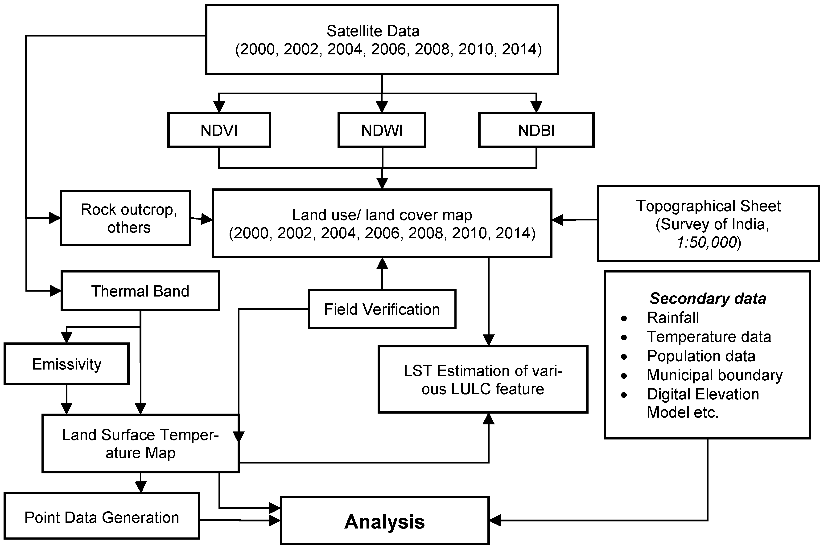
In this study, thermal bands from the LANDSAT series satellite were used to analyze the land surface temperature variability of Ranchi for the recent 14-year period from 2000 to 2014. The land use/land cover (LULC), LST, and UHI intensity in Ranchi were estimated using LANDSAT 5 TM (2002, 2004, 2006, 2008, and 2010), LANDSAT 7 ETM⁺ (2000 and 2002) and LANDSAT 8 OLI (2014) images, which were acquired from the United States Geological Survey (USGS, https://earthexplorer.usgs.gov/ (accessed on 20 February 2022);

Table 1. LANDSAT Data acquisition date and time.

Sensor	Acquisition Date	Time
ETM+	7 May 2000	10:05 a.m.
ETM+	13 May 2002	10:02 a.m.
TM	10 May 2004	09:53 a.m.
TM	16 May 2006	10:05 a.m.
TM	5 May 2008	10:02 a.m.
TM	11 May 2010	10:04 a.m.
TIRS	6 May 2014	10:12 a.m.

Path 140 and Row 44. Source: https://earthexplorer.usgs.gov/ (accessed on 20 February 2022).

). The spatial resolution of the thermal bands of LANDSAT TM was resampled at 30 m to maintain uniformity with LULC. The multispectral images LANDSAT TM and LANDSAT ETM⁺ (spectral bands 1 to 5 and 7) and LANDSAT 8 (spectral bands 2–7) were used to deduce urban land use and land cover based on indices such as NDVI, NDBI, and NDWI. Bands 6 of LANDSAT TM, bands 61 and 62 of LANDSAT ETM⁺, and bands 10 and 11 of LANDSAT 8 were used to retrieve land surface temperature (Figure 2).

2.1. Land-Use/Land-Cover Delineation

For the quantitative characterization of temporal and spatial vegetation patterns, Normalized Differential Vegetation Indices (NDVI) were used. Vegetation information in remote sensing is enhanced by rationing a near-infrared (NIR) band to a red (R) band, which capitalizes on the high vegetation reflectance in the NIR spectral range and the high pigment absorption of red light. NDVI was calculated using Equation (1). Normalized Difference Water Index (NDWI) was used to delineate open-water features using Equation (2). This index enhances the water features because of positive values for green light wavelengths, while vegetation and soil are suppressed (low reflectance of NIR) due to having zeroed or negative values. In NDWI, output was noisy since built-up land also has positive values in NDWI-derived images. The built-up land was extracted using the Normalized Difference Built-up Index (NDBI) following Zha et al. (2003) [57] using Equation (3). The development of the index was based on the unique spectral response of built-up land that has higher reflectance in the MIR wavelength range than in the NIR wavelength range. Even vegetation has a higher reflectance in MIR than in NIR, resulting in positive values in NDBI imagery for these plants, and water with highly suspended particles can also reflect MIR stronger than in NIR, resulting in positive values in NDBI.

NDVI = (ρNIR − ρR)/(ρNIR + ρR)

(1)

NDWI = (ρGREEN − ρNIR)/(ρGREEN + ρNIR)

(2)

NDBI = (ρMIR − ρNIR)/(ρMIR + ρNIR)

(3)

The respective thematic features, specifically vegetation, water bodies, and built-up areas, were extracted from indexed images using threshold values. The built-up land class includes constructed areas, specifically settlements, hamlets, residential colonies, industries, commercial, road, transportation junctions, etc. Vegetation comprised all land under tree cover, forest cover, agricultural cropland, and plantations. Water bodies cover surface water, including streams, rivers, and ponds. As bare rocks had a significant role in LST, they were separately delineated as exposed rocks. The remaining areas, which were not covered in the above LULC classes, were classified as “other”. All the individual LULC classes were merged to prepare land-use/land-cover maps, which were verified during the selective field verification conducted in May 2016 using Google Earth images. The field information was used to update the LULC map and conduct further analysis.

2.2. Land Surface Estimation

The digital number (DN) of LANDSAT TM/ETM⁺/LANDSAT 8 is converted into spectral radiance using Equation (4) following Chander and Markham, 2003 [58]. The reflectance of each band of LANDSAT TM/ETM⁺/LANDSAT8 is estimated using Equations (5) and (6).

L = Gain × DN + Bias

(4)

ρ = (∏Ld²)/(ECosθ) for LANDSAT TM/LANDSAT ETM⁺

(5)

$$\mathsf{\rho }=\left(\mathrm{L}\right)/\left(\mathrm{ECos}\mathsf{\theta }\right)=(\mathrm{L})/(\mathrm{ESin}\mathsf{\theta }) \mathrm{for} \mathrm{LANDSAT}8$$

(6)

where Gain and Bias value. L = Spectral Radiance from the above equation, d = Earth-sun Distance in the astronomical unit, θ = Sun zenith angle (which is provided in the metadata file), and E = Exo-atmospheric solar irradiance.

To convert DNs to the actual temperature values, a two-step process was adopted: (a) conversion of DNs values to spectral radiance values, following Equations (7) and (8); (b) conversion of spectral radiance to sensor brightness temperature in Kelvin, following Equation (9). conversion of DNs values to spectral radiance values

L = (L_MAX − L_MIN) × DN/255 + L_MIN (for LANDSAT TM/ETM⁺)

(7)

L = (L_MAX − L_MIN) × DN/65535 + L_MIN (for LANDSAT 8)

(8)

Alternatively, it can be written as:

L = Gain × DN + Bias

where L = spectral radiance, L_MIN = (1.238 for LANDSAT 5 TM and 0.0 for band 6_1 and 3.2 for band 6_2 for LANDSAT ETM⁺ and 0.10033 for LANDSAT 8 Band 10,11), L_MAX = (15.303 for LANDSAT 5 TM and 17.040 for band 6_1 and 12.650 for band 6_2 for LANDSAT 7 ETM⁺ and 22.00180 LANDSAT 8 Band 10, 11). The conversion of spectral radiance to sensor brightness temperature in Kelvin was performed using the following equation.

T_SENSOR = (K2)/ln(K1 × εL + 1)

(9)

where T_SENSOR = effective at-satellite temperature in Kelvin, K2 = calibration constant (607.76 for LANDSAT 5 TM and 666.09 for LANDSAT 7 ETM⁺) and 1321.08 and 1201.14 for LANDSAT 8 band 10 and 11, respectively, K1 = calibration constant (1260.56 for LANDSAT 5 TM and 1282.71 for LANDSAT 7 ETM⁺) and 774.89 and 480.89 for LANDSAT 8 band 10 and 11, respectively, L = spectral radiance in watt/(meter squared × ster × m), ε = Emissivity.

Spectral emissivity (ε) is required to account for the non-uniform emissivity of the land surface. The spectral emissivity for all objects is very close to 1, yet for more accurate temperature derivation, the emissivity of each land-cover class is considered separately. Emissivity correction is carried out using surface emissivity for the specified land covers (

Table 2. Area statistics of LULC from 2000 to 2014 (units are in sq. km).

LULC Class	2000	2002	2004	2006	2008	2010	2014	Total Change 2000–2014
Built-up	35.38	37.04	41.98	43.70	44.06	60.71	83.03	47.65
Water body	26.40	23.81	26.90	26.82	26.26	25.12	30.67	4.27
Vegetation	334.59	370.19	614.57	497.51	142.35	283.11	311.83	−22.76
Exposed rock	46.19	25.61	27.80	20.96	34.72	35.34	25.79	−20.4
Other	1074.16	1060.07	805.48	927.73	1269.33	1112.45	1065.40	−8.76
Total	1516.72	1516.72	1516.72	1516.72	1516.72	1516.72	1516.72

and

Table 3. Percentage (%) change in LULC during 2000–2014 (units are in %).

LULC	2000–2002	2002–2004	2004–2006	2006–2008	2008–2010	2010–2014	2000–2014
Built-up	4.69	13.34	4.10	0.82	37.79	36.76	135.00
Water body	−9.81	12.98	−0.30	−2.09	−4.34	22.09	16.17
Vegetation	10.64	66.01	−19.05	−71.39	98.88	10.15	−6.80
Exposed rock	−44.56	8.55	−24.60	65.65	1.79	−27.02	−44.16
Other	−1.31	−24.02	15.18	36.82	−12.36	−4.23	−0.81

), following Snyder et al. (1998) [59] and Stathopoulos and Cartalis (2009) [29]. To retrieve the land surface emissivity-corrected temperature data, the Kelvin temperature was converted into the Celsius scale using Equation (10).

T_C = T_SENSOR − 273 °C

(10)

where T_C = temperature in Celsius.

After retrieving LST, it was reclassified into various classes, specifically very low (<26 °C), low (24–30 °C), moderate (30–34 °C), moderately high (34–38 °C), very high (38–42 °C), and severely high (>42 °C) to estimate the area and its spatial relationship with different LULC. The derived LST was correlated with different Cartosat I-based relief zones as well as with LULC in the urban and peri-urban regions to assess the altitudinal variation of LST and its impact on the landscape phenomenon.

3. Results

Multi-temporal satellite observations were used to map land use/land cover and land surface temperature variability from 2000 to 2014 every two consecutive years. The LULC and LST datasets were analyzed through various geospatial and statistical methods to comprehend the thermal variability of haphazardly growing Ranchi urban and peri-urban regions.

3.1. Land Transformation

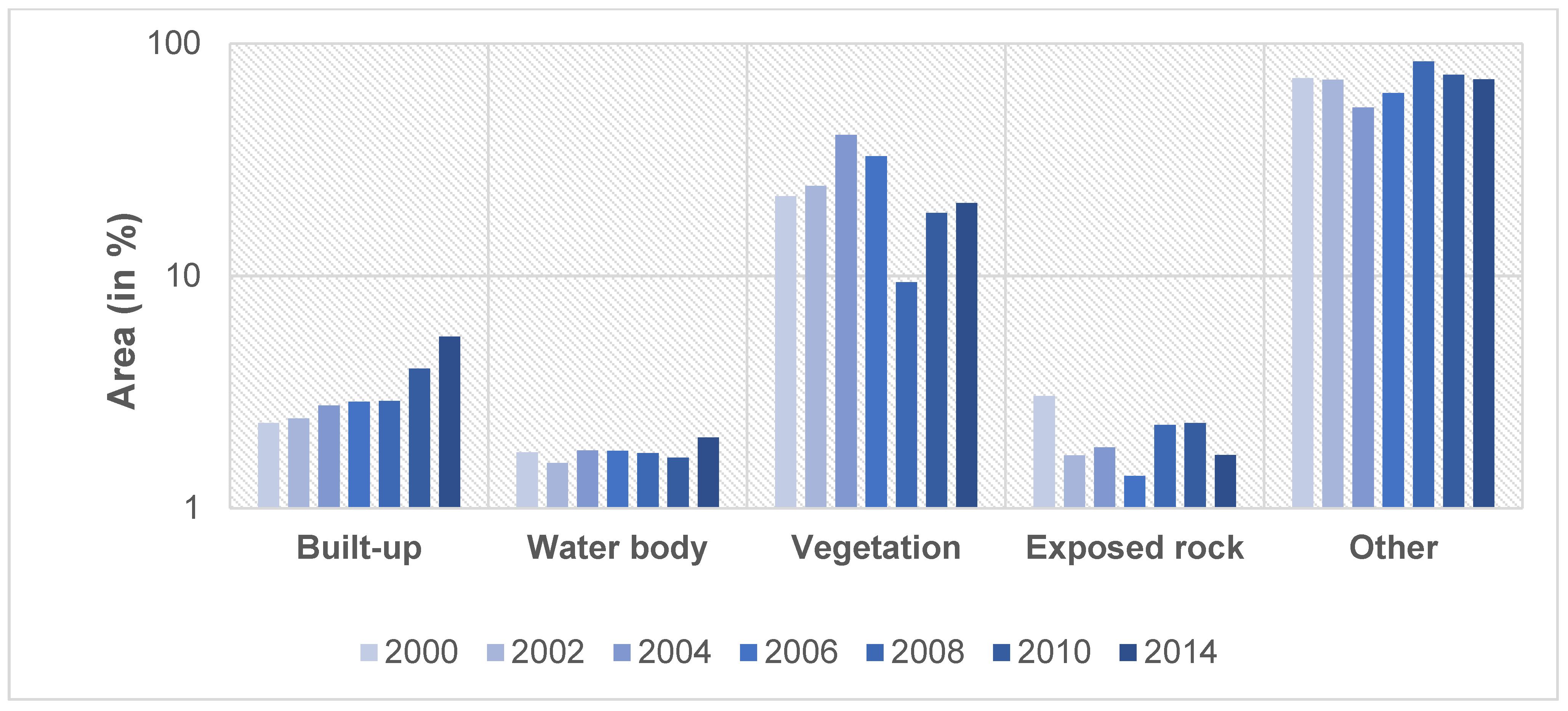
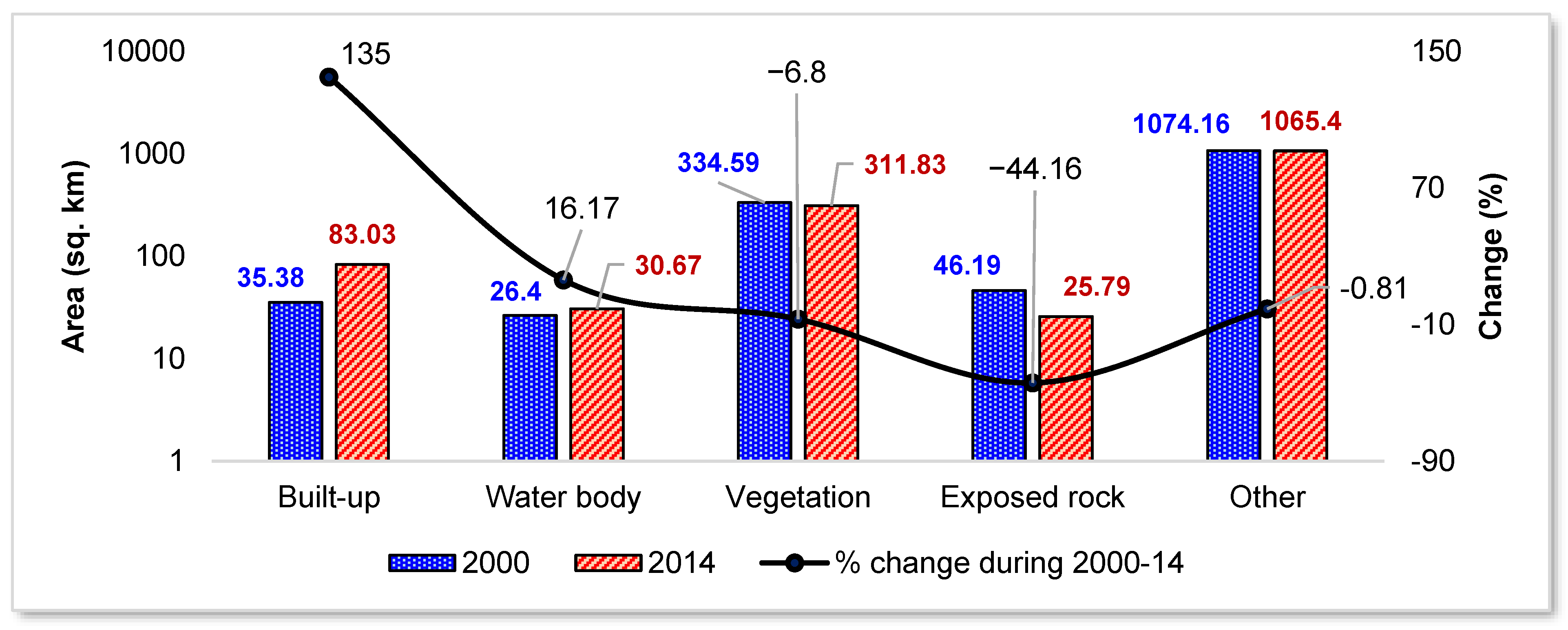
Spatiotemporal LULC changes in Ranchi’s urban and peri-urban regions were performed from 2000 to 2014 on a bi-annual basis using the LANDSAT satellite. The satellite-based observations exhibited a gradual increase in built-up areas in RUA, with a net growth of 47.65 sq. km (with 135% growth) from 2000 to 2014 (Table 2 and Table 3). The built-up area was 35.38 sq. km in 2000 and increased to 37.04 sq. km (4.69%) in 2002, 41.98 sq. km (13.34%) in 2004, 43.98 sq. km (4.10%) in 2006, 44.06 sq. km (0.82%) in 2008, 60.71 sq. km (37.79%) in 2010, and 83.03 sq. km (36.76%) in 2014. Significant built-up land growth was observed in the north (Kanke), northeastern (Booti More), and northwestern parts (Nagri), which influence the irreversible alteration of the other LULC classes (Figure 3 and Figure 4). The rapid built-up land growth is linked to the change in socioeconomic status, implementation of government development projects, and other interventions during post-2000 periods due to the reorganization of Ranchi as the state capital in 2000 [55,60].

Spatiotemporal LULC mapping exhibited a decrease in vegetation cover of 22.76 sq. km (−6.80%) from 2000 to 2014 (Table 2 and Table 3), which is attributed primarily to encroachment by built-up areas. The vegetation cover decreased to 497.51 sq. km (−19.05%) in 2006 and to 142.35 sq. km (−71.39%) in 2008. By contrast, there was an increase in vegetation cover in the years 2010 (283.11 sq. km, 98.88%) and 2014 (311.83 sq. km, 10.15%). The significant increase in vegetation cover in 2004 as compared to 2002 may be due to the early arrival of the monsoon in 2004, which might have favored the vegetation growth (including grass, shrubs, trees, etc.) in the satellite image [61]. Although the water body and exposed rock had less coverage in RUA, nominal episodic increases and decreases were observed throughout the observation periods. The waterbody increased from 26.40 sq. km to 30.67 sq. km (16.17%) from 2000 to 2014. The periodic observation reveals that the water body occupied 26.40 sq. km in 2000 and decreased to 23.81 sq. km in 2002 with a decline of 9.81% (mainly in the Getalsud reservoir); a minor decrease of 0.30% was evident in 2006 (26.82 sq. km), −2.09% in 2008 (26.26 sq. km), and −4.34% in 2010 (25.12 sq. km), except for 2004 and 2014, with an increase of 26.90 sq. km (12.98%) to 30.67 sq. km (22.09%). Exposed rock had an almost decreasing trend from 46.19 sq. km to 25.79 sq. km from 2000 to 2014 with an overall decrease of −44.16% (Table 2 and Table 3). Furthermore, an increase in the area of exposed rock was observed in 2004 (27.80 sq. km), 2008 (34.72 sq. km), and 2010 (35.34 sq. km), except for 2002 (25.61 sq. km), 2006 (20.96 sq. km), and 2014 (25.79 sq. km). The episodic increase and decrease in the area of exposed rock could be attributed to the exposure of rocky areas, which are generally covered by vegetation due to the erratic pattern of precipitation in the region. Additionally, prevalent rock-mining activity in the region in recent years has led to the exposure of rocky outcrops. The area of exposed rocks generally falls into other or vegetation classes during the observation periods due to its mixed surface reflectance. The area of the “other” class (mainly including bare soil and fallow land) showed a decreasing trend from 2000 to 2014 (−0.81%). There was a periodic decline of bare soil and fallow land in 2002 (1060.07 sq. km) and 2004 (805.48 sq km). Moreover, a gradual increase was observed from 2006 (927.73 sq. km) to 2008 (1269.33 sq. km), except for 2010 (1112.45 sq. km) and 2014 (1065.40 sq. km).

The spatiotemporal pattern of LULC dynamics during the period 2000–2014 exhibits unprecedented built-up growth from 35.38 sq. km to 83.03 sq. km (135%) due to high population growth (461.09%; 844,000 to 1,232,000 people from 2000 to 2014), which is influenced by a change in the political-socio-economic condition of Ranchi (Figure 3, Figure 4 and Figure 5). On the contrary, a decrease in the spatial extent of vegetation, exposed rocks, and other classes was observed [62], while an increase in the area of the water bodies was apparent in the region during the 2000–2014 period.

3.2. Periodic Variability in Land Surface Temperature

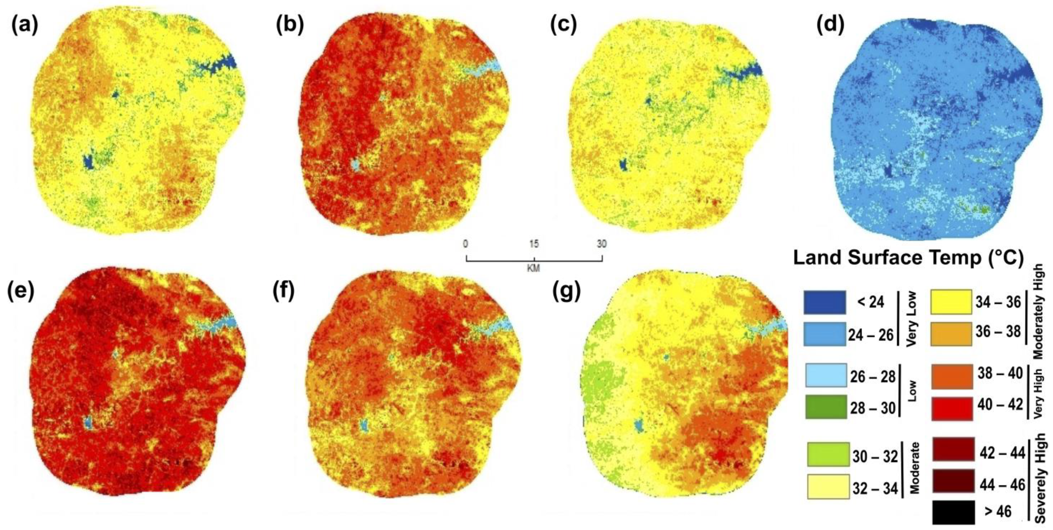
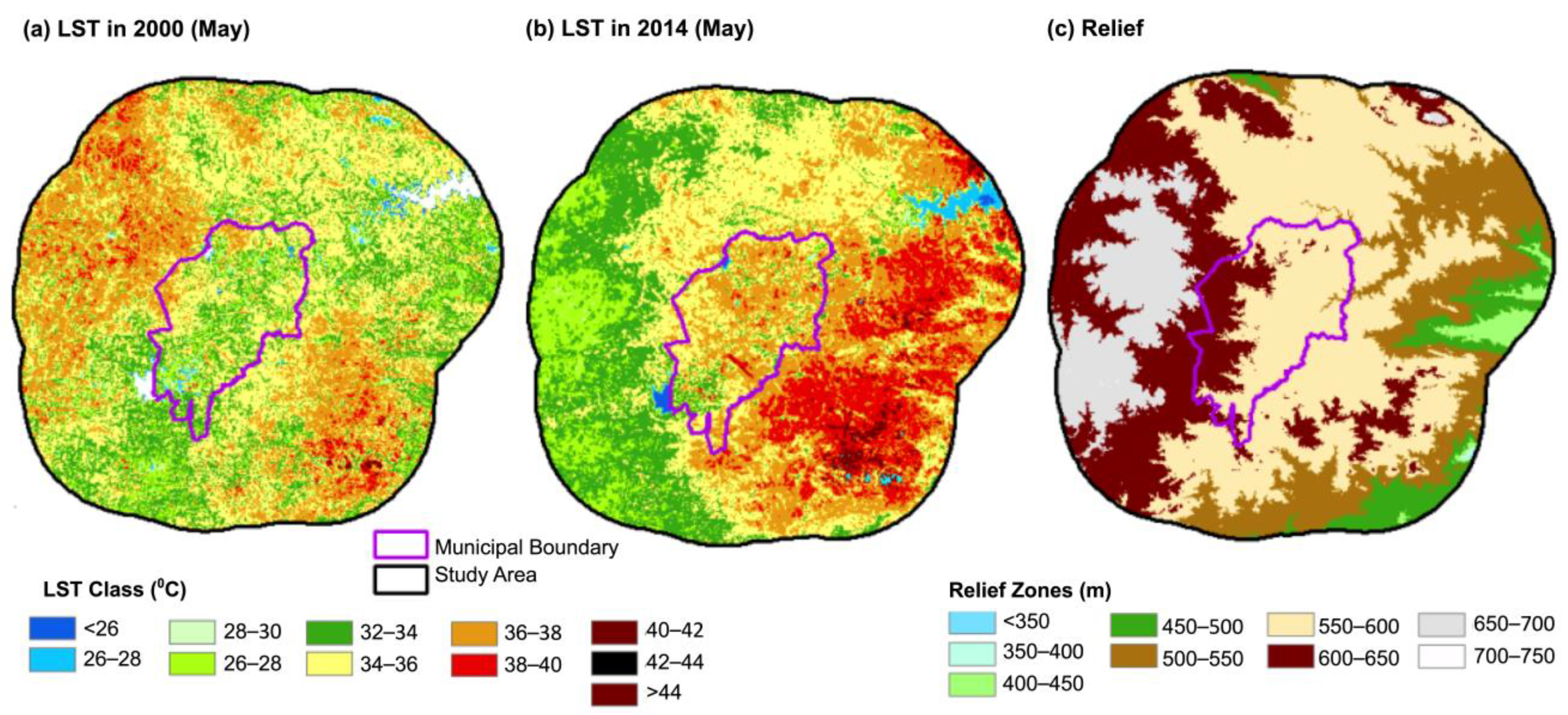
The LST was analyzed for all the observation years during May 2000, 2002, 2004, 2006, 2008, 2010, and 2014 using LANDSAT thermal satellite images (Figure 6a–g). The LST exhibited an increasing trend during the observation period, except for 2004 and 2006. For 2000, LST ranged from moderately high (36 °C to 38 °C) in northwestern and southeastern parts occupying exposed rock surfaces and fallow/uncultivated agricultural land to very low (22 °C to 26 °C) for water bodies. Moreover, RUA accounts for 22 °C to 44 °C of LST, where built-up land is mainly located in the central part of RUA, which has moderate to moderately high LST (32 °C to 36 °C). In 2002, the LST values ranged from 26 °C to 46 °C where vegetated cover was depicted as moderately high LST (34 °C to 36 °C) in the north and northeastern parts of RUA, built-up land was moderately high to high (36 °C to 40 °C) and water bodies with very low to low LST (24 °C to 28 °C). The north-west and south-west, consisting mainly of non-vegetated surfaces (bare soil and fallow land), had very high LST (40 °C to 42 °C), whereas exposed rock exhibited very high and severely high LST (40 °C to 44 °C).

During May 2004, lower LST was observed, which ranged from 22 °C to 42 °C due to rainfall occurrence before the satellite image acquisition. Similarly, low LST (15 °C to 33 °C) in 2006 was attributed to heavy rainfall in the morning hours on the same day. A very high LST (38 °C to 42 °C) was observed over exposed rock (southeastern parts), while the LST over bare soil or uncultivated land in the southwestern part was in a moderate and moderately high LST zone (34 °C to 38 °C). The central part, mainly comprising urban built-up land, exhibited moderate to moderately high LST (32 °C to 36 °C). In contrast, in 2006, it was seen that due to rainfall, there was a wide variation in temperature throughout the region. Almost all features exhibited low LST except for the built-up land located in the center parts, where LST ranged from 24 °C to 28 °C (very low to low LST), and in the southeastern parts, which primarily consisted of exposed rock, where LST ranged from 30 °C to 32 °C (low to moderate LST).

The highest LST in Ranchi was recorded in May 2008, ranging from 24 °C to 48 °C. The central parts comprised of built-up land had moderately high to very high LST (34 °C to 40 °C), whereas the exposed rocks in the region exhibited severely high LST (44 °C to 48 °C), and water bodies had the lowest LST (26 °C to 28 °C). During May 2010, the LST ranged from 25 °C to 47 °C, with the major parts including the central built-up area, the northern vegetated area, the southeastern uncultivated and vegetated area, and the southwestern uncultivated area having a moderate to moderately high LST (34 °C to 38 °C). Meanwhile, the northeastern parts (the uncultivated area), southeastern (exposed rocks), and northwestern (uncultivated land with rock outcrops) showed very high to severely high LST (40 °C to 46 °C).

The LST of the water body was lowest compared to the remaining LULC classes and ranged between 24 °C and 28 °C. The highest LST in Ranchi was recorded in May 2008, ranging from 24 °C to 48 °C. The central parts comprised of built-up land had moderately high to very high LST (34 °C to 40 °C), whereas the exposed rocks in the region exhibited severely high LST (44 °C to 48 °C), and water bodies had the lowest LST (26 °C to 28 °C). During May 2010, the LST ranged from 25 °C to 47 °C, in which the major parts including the central built-up area, northern vegetated area, southeastern uncultivated and vegetated area, and the southwestern uncultivated area had moderate to moderately high LST (34 °C to 38 °C). Meanwhile, the northeastern parts (the uncultivated area), southeastern (exposed rocks), and northwestern (uncultivated land with rock outcrops) had very high to severely high LST (40 °C to 46 °C). The LST of the water body was lowest as compared to the remaining LULC classes and ranged between 24 °C and 28 °C. In May 2014, the LST ranged from 26 °C to 46 °C. It is emphasized that even after an overnight rainfall, the LST was very high to severely high in southeastern parts (38 °C to 46 °C), mainly comprised of rock outcrops and uncultivated land. However, the majority of the area had moderate to moderately high LST (32 °C to 36 °C), whereas the central built-up area has moderately high LST (36 °C to 38 °C), and the southwestern area with moderate LST (30 °C to 32 °C). Water bodies had the lowest LST, ranging between 26 °C and 28 °C. The land surface temperature variability in Ranchi throughout the observation period exhibited a significant increase. A similar study was conducted depicting the physiographic characteristics of different land covers to LST where exposed rocks, fallow, and bare soil are classified as high LST zones in contrast to the water body and vegetation [53].

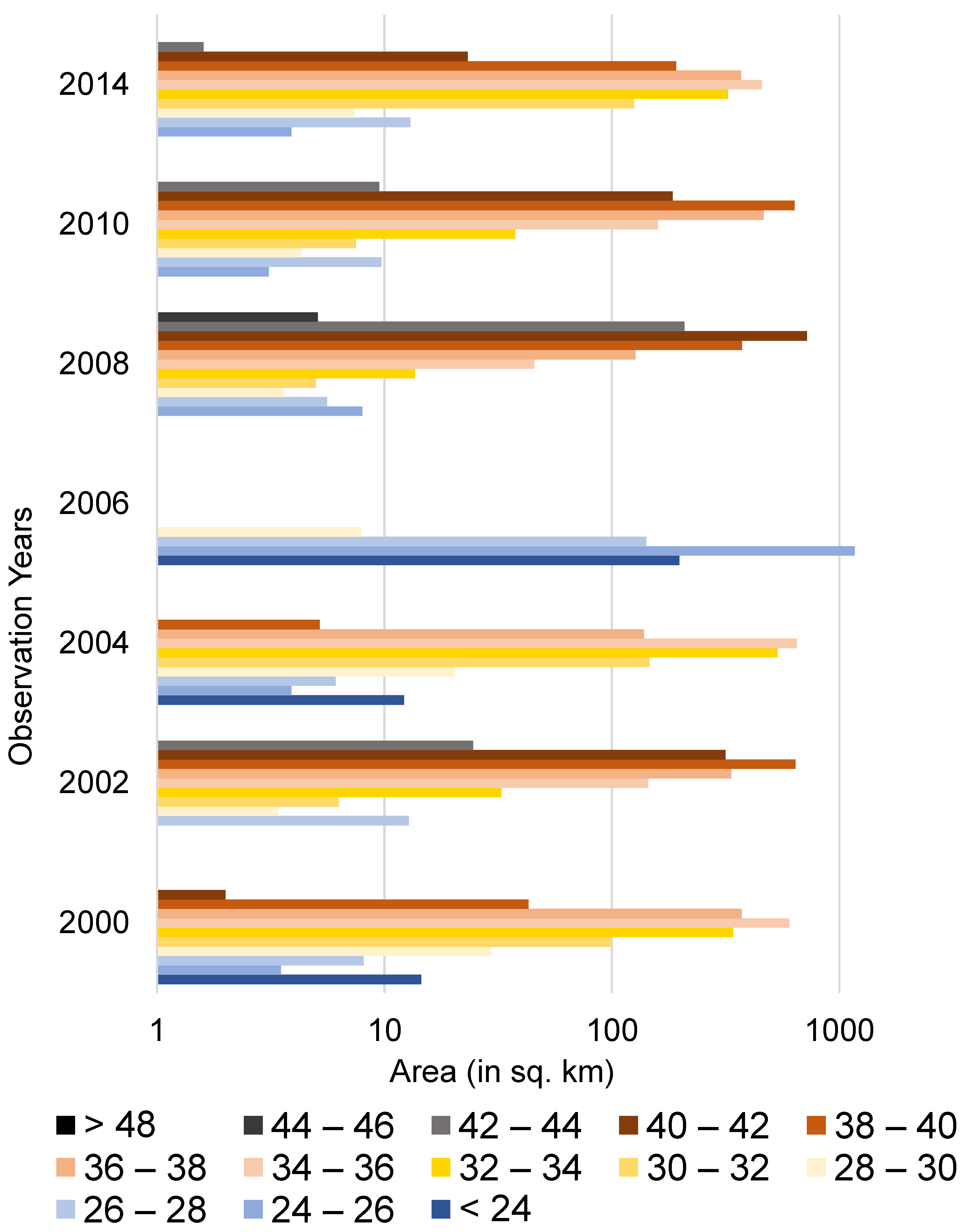
3.3. Spatial Variability of LST in RUA from 2000 to 2014

The spatial patterns of LST were studied and analyzed from 2000 to 2014 after every consecutive year. The LST zone was classified into three major classes, namely low (<30 °C), moderate (30 °C to 38 °C), and high (>38 °C) (Figure 6 and Figure 7;

Table 4. Area statistics of land surface temperature zones during 2000-14 (Units are in sq. km).

LST Zone	LST (°C)	2000	2002	2004	2006	2008	2010	2014
Low	<24	14.5	0.0	12.2	198.2	0.0	0.0	0.0
	24–26	3.5	1.0	3.9	1168.9	8.0	3.1	3.9
	26–28	8.1	12.8	6.1	141.7	5.6	9.7	13.0
	28–30	29.5	3.4	20.4	7.9	3.6	4.3	7.4
Moderate	30–32	98.8	6.3	146.0	0.0	5.0	7.5	125.4
	32–34	341.0	32.7	534.1	0.0	13.6	37.5	324.0
	34–36	604.6	144.1	650.6	0.0	45.5	159.6	456.7
	36–38	371.9	335.0	138.2	0.0	126.8	464.7	370.0
High	38–40	42.9	641.0	5.2	0.0	373.5	635.4	191.6
	40–42	2.0	315.9	0.0	0.0	721.6	184.7	23.2
	42–44	0.0	24.5	0.0	0.0	208.3	9.5	1.6
	44–46	0.0	0.2	0.0	0.0	5.1	0.7	0.0
	>48	0.0	0.0	0.0	0.0	0.3	0.0	0.0

and

Table 5. Summarized area statistics of LST zones in RUA and environs during 2000–2014.

LST Zone	LST (°C)	2000	2002	2004	2006	2008	2010	2014
(Units are in sq. km)
Low	<30	55.5	17.1	42.6	1516.7	17.2	17.1	24.3
Moderate	30–38	1416.4	518.0	1468.9	0.0	190.8	669.3	1276.1
High	38–48	44.9	981.6	5.2	0.0	1308.8	830.3	216.3
Units are in %
Low	<30	3.7	1.1	2.8	100.0	1.1	1.1	1.6
Moderate	30–38	93.4	34.2	96.8	0.0	12.6	44.1	84.1
High	38–48	3.0	64.7	0.3	0.0	86.3	54.7	14.3

). The majority of the area was in the moderate LST zone during 2000 (93.4%), 2004 (96.8%), and 2014 (84.1%) except for 2002(64.7%), 2008 (86.3%), and 2010 (54.7%) under the high LST zone. The low LST (<30 °C) zone covered 55.5 sq. km (3.7%) of an area in 2000, which decreased to 17.1 sq. km (1.1%) in 2002 and later increased to 42.30 sq. km (2.8%) in 2004. The low LST zone was 17.2 sq. km (1.1%) in 2008, 17.1 sq. km (1.1%) in 2010, and 24.3 sq. km (1.6%) in 2014. The moderate LST (30 °C to 38 °C) zone covered 1416.4 sq. km (93.4%) in 2000 which decreased to 518.0 sq. km (34.2%) in 2002 and later increased to 1468.85 sq. km (96.8%) in 2004. The moderate LST zone was null in 2006 due to low LST, which increased to 190.8 sq. km (12.6%) in 2008, 669.3 sq. km (44.1%) in 2010, and 1276.1 sq. km (84.1%) in 2014. The high LST (>38 °C) zone covered 44.9 sq. km (3.0%) in 2000, which increased to 981.6 sq. km (64.7%) in 2002, and later reduced to 5.2 sq. km (0.3%) and null in 2006. It increased to 1308.8 sq. km (86.3%) in 2008 and later reduced to 830.3 sq. km (54.7%) and 216.3 sq. km (14.3%) in 2014. It was observed that in summer (May), the urban fringe and neighboring rural regions were warmer than the core urban area due to the existence of rock outcrops and non-cultivated agricultural land (fallow land) [53,54,55,56,57,58,59,60] (Figure 6 and Figure 7; Table 4 and Table 5). The increase in the urban trajectory of the study area quantifies its thermal behavior [63]; although the LST was distinctively escalating during May, the urban area was cooler than its environs from 2000 to 2014 except for 2006. Similarly, spatiotemporal LST variability from 2000 to 2014 exhibited an increase in area under higher temperature zones, except for 2006, where cooling occurred due to heavy rainfall.

3.4. Influence of LULC Change on Land Surface Temperature

The LST and land-use/land-cover variables were spatially correlated to deduce the LST characteristics of each land surface feature and its dynamics from 2000 to 2014. During May 2000, the LST ranged from 22 °C to 44 °C, whereas during May 2014, it ranged from 26 °C to 46 °C. During both periods, the estimated highest surface temperature mainly existed over the exposed rocky area and in the non-cultivated agricultural lands located in the urban fringe. On the contrary, the cooler areas were mainly associated with water bodies and vegetation.

The correlation exhibited that the LST of all the LULC classes increased from 2000 to 2014 (

Table 6. Land-use/land-cover relationship with LST (2000–2014).

LST (°C)	Built-Up Land		Water Body		Vegetation		Rock Outcrop		Other		Total Area
	2000	2014	2000	2014	2000	2014	2000	2014	2000	2014	2000	2014
Units are sq. km
<30	0.09	0	20.99	20.3	32.98	3.66	0.03	0	1.41	0.26	55.5	24.22
30 to 38	34.96	74.79	5.4	10.3	301.6	303.34	35.53	9.76	1038.79	877.94	1416.28	1276.13
38 to >48	0.33	8.25	0.01	0.07	0.01	4.88	10.64	15.94	33.96	187.16	44.95	216.3
Units are % of a particular class of observation year
<30	0.25	0.00	79.51	66.19	9.86	1.17	0.06	0.00	0.13	0.02	3.66	1.60
30 to 38	98.81	90.07	20.45	33.58	90.14	97.26	76.90	37.98	96.71	82.41	93.38	84.14
38 to >48	0.93	9.93	0.04	0.23	0.00	1.56	23.03	62.02	3.16	17.57	2.96	14.26
% change in LULC area coverage under varied LST zones from 2000 to 2014
LST (°C)	Built-up Land		Water Body		Vegetation		Rock Outcrop		Other		Total Area
<30	−100.0		−3.3		−88.9		−100.0		−81.6		−56.4
30 to 38	113.9		90.7		0.6		−72.5		−15.5		−9.9
38 to >48	2400.0		600.0		48700.0		49.8		451.1		381.2

). During May 2000, most of the built-up land (34.96 sq. km; 98.8% of total built-up area) was under moderate LST (30 °C to 38 °C) zone, whereas very insignificant built-up land (0.33 sq. km; 0.9%) was under high LST (>38 °C). During May 2014, most of the built-up land (74.79 sq. km; 90.1%) was under a moderate LST zone followed by a high LST zone (8.25 sq. km; 9.9% of built-up land). During May 2000, the majority (301.6 sq. km; 90.1%) of vegetation cover was under moderate LST zone followed by low LST (32.9 sq. km; 9.9%). During 2014, the majority (303.4 sq. km; 97.3%) of vegetation cover was under moderate LST zone followed by an insignificant 4.8 sq. km (1.6%) under high and 3.6 sq. km (1.2%) under low LST zone. During May 2000, the (35.5 sq. km; 76.9%) of rock outcrop was under a moderate LST zone followed by a significant 10.6 sq. km (23.0%) under a high LST zone. During 2014, the majority (15.94 sq. km; 62.0%) of rock outcrop was under a high LST zone followed by a moderate LST zone (9.76 sq. km; 38%). The “other” class was under a moderate LST zone in the majority (1038.8 sq. km; 96.7%) of areas followed by a high LST zone (33.96 sq. km; 3.2%) during 2000. During 2014, the majority (877.94 sq. km; 82.4%) of the area under the “other” class was under the moderate LST zone followed by a high LST zone (187.16 sq. km; 17.6%).

The percentage change in LULC area coverage under varied LST zones from May 2000 to May 2014 exhibits a substantial increase in all land-use features under high LST (381%) followed by low LST (−56.4%), and moderate LST (−9.9). The negative change signifies loss of area under low LST and moderate LST zone due to an increase in near-surface temperature of varied LULC classes and the gradual shift of near-surface temperature to moderate and high LST zone, respectively.

The maximum percent change was observed in vegetation cover, wherein the area of the high LST zone was raised from 0.01 sq. km to 4.88 sq. km from 2000 to 2014. This may be attributed to the degradation in vegetation cover primarily located in the hilly area and in the vicinity of exposed rock, which influences the heat in the degraded/low dense vegetation cover. The second most substantial percentage change was observed in the built-up area, wherein the area under the high LST zone increased from 0.33 sq. km to 8.25 sq. km from 2000 to 2014. Additionally, the percentage change in the low LST area was null and shifted to a higher temperature leading to an increase in moderate LST built-up area. The high LST of the water body increased from 0.01 sq. km to 0.07 sq. km from 2000 to 2014, whereas the moderate LST water body increased from 5.4 sq. km to 10.3 sq. km with 90.7%. The low LST in the water body was reduced by 3.3%. The high LST in the “other” class also increased from 33.96 sq. km to 187.16 sq. km from 2000 to 2014 with 451.1%. On the contrary, moderate LST in the “other” class area was reduced from 96.71 sq. km to 82.41 sq. km (−15.5%) and low LST from 1.41 sq. km to 0.26 sq. km (−81.6%). The high LST in the rock outcrop area increased from 10.64 sq. km to 15.94 sq. km (49.8%). Meanwhile, the moderate LST in rock outcrop decreased from 35.53 sq. km to 9.76 sq. km (−82.5%) and low LST from 0.03 sq. km to null area (−100%).

The results show the increase in surface temperature in all land-use/land-cover classes in RUA from 2000 to 2014, particularly in vegetation, built-up land, and water bodies. Although LST is a local phenomenon, it is highly influenced by adjoining land use. The high presence of rock outcrop in the plateau topography, uncultivated land, and vegetation in hilly/rocky areas is the major controlling factor of LST in the region, and a high positive correlation is estimated between LST and built-up land and low compared with water bodies [64]. The study shows that a heat island is not formed properly over Ranchi urban area though the surface temperature of built-up land increased over the periods (2000–2014). In conformity with the present report, Ren et al., (2009) reported a similar urban microclimate warming effect in China, where both rural and urban areas experienced a rapid temperature increase over time.

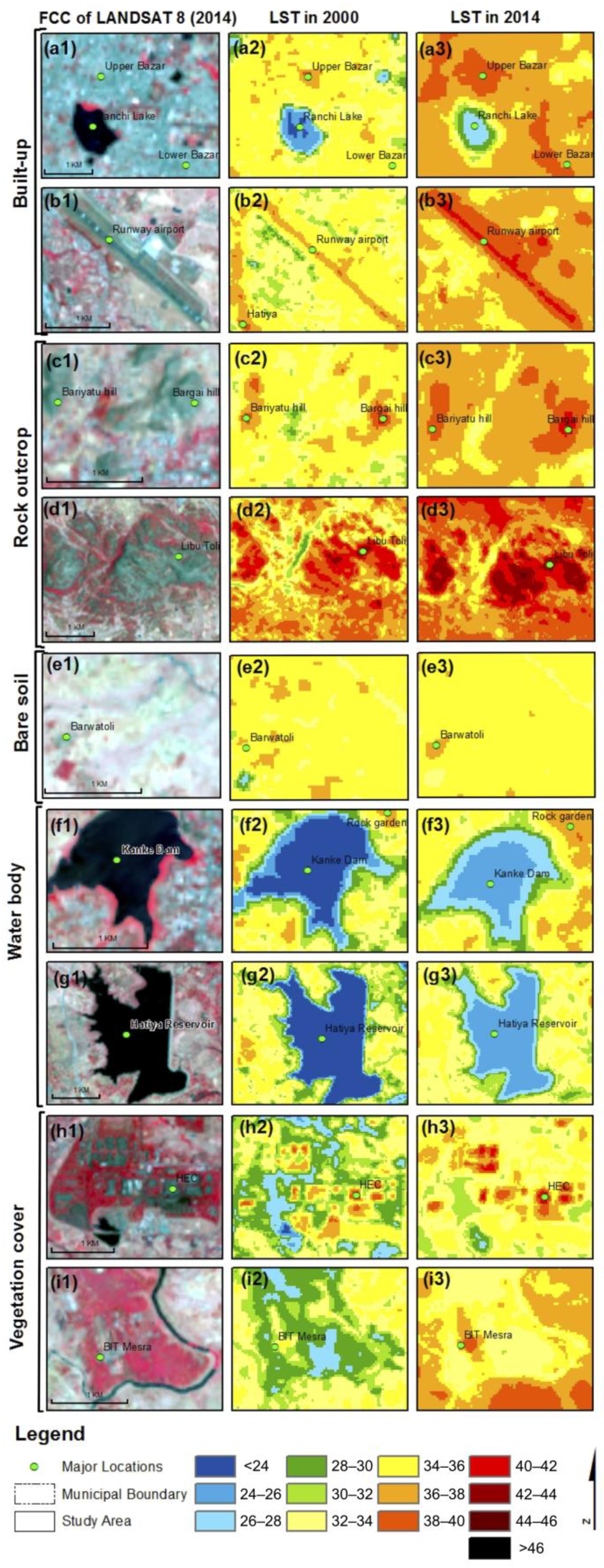
3.5. Analyzing Heat Islands vs. Heat Sinks in Urban and Peri-Urban Regions

LST maps for the years 2000 and 2014 were used to comprehend the spatiotemporal LST patterns at the urban scale with reference to land-use/land cover in Ranchi urban and peri-urban regions. The study exhibits that the RUA is characterized by a series of “heat islands” and “heat sinks” at a local level (Figure 8). A distinct temperature gradient was evident, with the coolest temperatures on the water bodies followed by vegetation cover. Although the surface temperature of the water bodies increased from 2000 to 2014, it remained less than 26 °C (Figure 8a,f,g). These land surface features with distinctive low surface temperature act as “heat sinks” and are primarily related to major lakes and reservoirs [65]. The LST of the vegetation cover was comparatively higher and increased over the periods. It ranged from 26 to 32 °C in 2000 and from 30 to 36 °C in 2014 (Figure 8h,i). The LST of the built-up area was conspicuously higher and increased over the periods. It ranged between 34 and 38 °C during 2000 and between 36 and 42 °C in 2014 (Figure 8a,b,h), showing the built-up area as an urban heat island at the local level with increasing surface temperature. The LST of the exposed rock was significantly higher and ranged between 36 and 44 °C during 2000 and between 38 and 46 °C during 2014 (Figure 8c,d). The LST of uncultivated agricultural land also exhibited higher LST and ranged between 32 and 36 °C during 2000 and between 34 and 38 °C in 2014 (Figure 8e,i). This represents the select land feature as a heat island at a local scale with increasing surface temperature over the years. The average surface temperature study exhibits that the vegetation cover has a higher average surface temperature than water bodies, but a lower average surface temperature as compared to the remaining LULC class. The area with dense vegetation and distant from exposed rock has low to moderate LST (28 °C to 32 °C). In accordance with the present analysis, a similar study has been conducted to identify the heat source and heat sink zones in central China where low LST values among the urban areas are confined due to the presence of vegetation cover [66].

The urban area is a conglomeration of varied land surface features, and each feature within the urban region has a different thermal region. The dense built-up area and exposed rock enable the formation of urban heat islands; water bodies and vegetation cover enable the formation of macro-level cool islands/heat sinks in the urban region. At a regional level, the spatiotemporal LST study showed lower LST in the urban region as compared to its environs, due to the rocky terrain in the vicinity. The urban area in RUA is not a continuous built-up zone and consists of vacant land and vegetation cover at various locations, as demonstrated by the high-resolution Google Earth satellite image, which was validated during the field visit. The past imposition of the Chhota Nagpur Tenancy (CNT) Act in the region has restricted the free movement of land ownership from tribal people to non-tribal people. Therefore, a major part of the land in the urban region remains vacant or undeveloped (non-impervious in nature), which contributes to minimizing the increasing land surface effect of the surrounding built-up (impervious) land. The built-up area in RUA is mainly surrounded by exposed rock, bare soil, and uncultivated land, mainly in the southeast and western parts, where the surface temperature is very high (44–46 °C). The absence of soil moisture or the presence of dry soil reduces thermal inertia to a greater extent and forms urban areas as urban cool islands due to the high LST in the peripheral region.

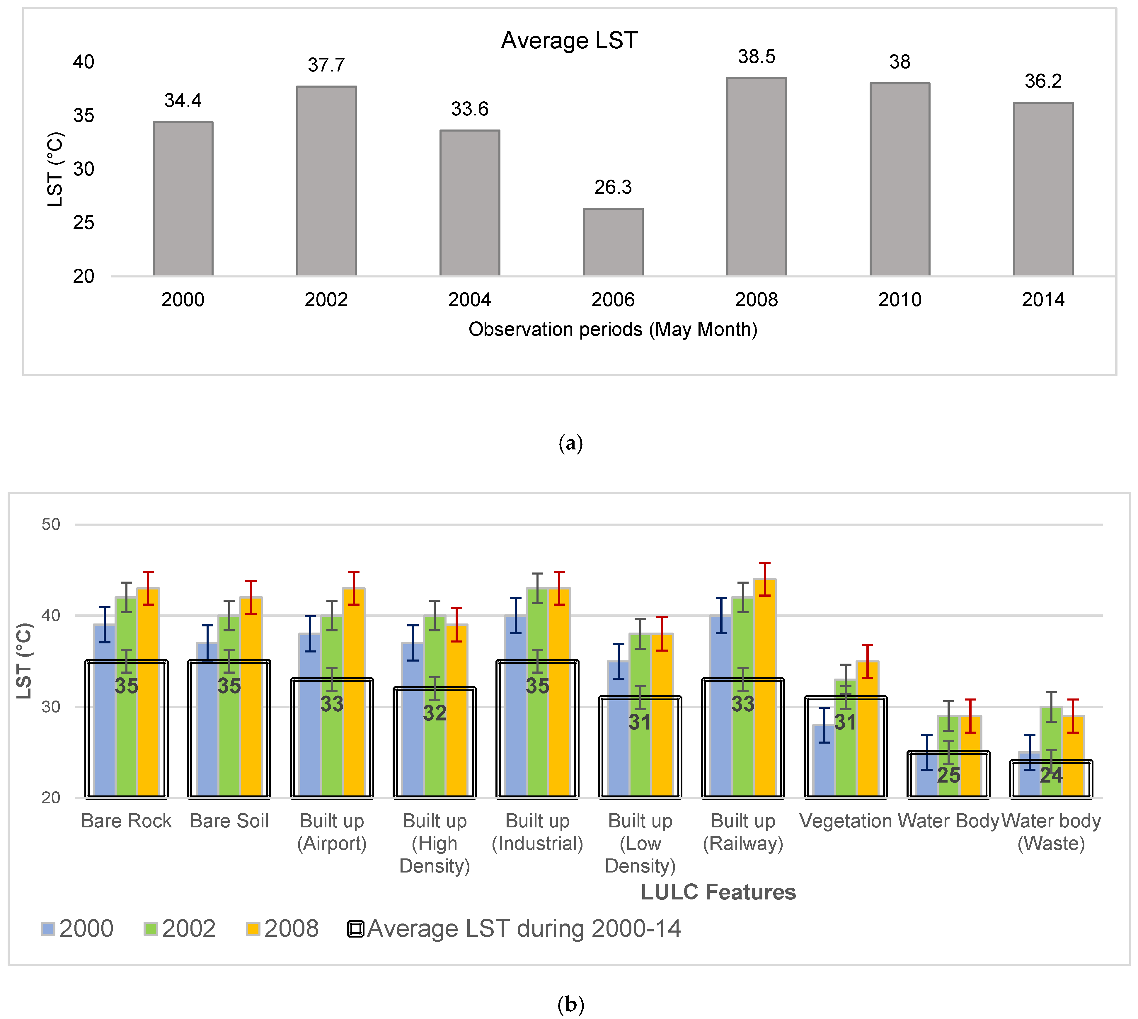
3.6. Land Surface Temperature Dynamics

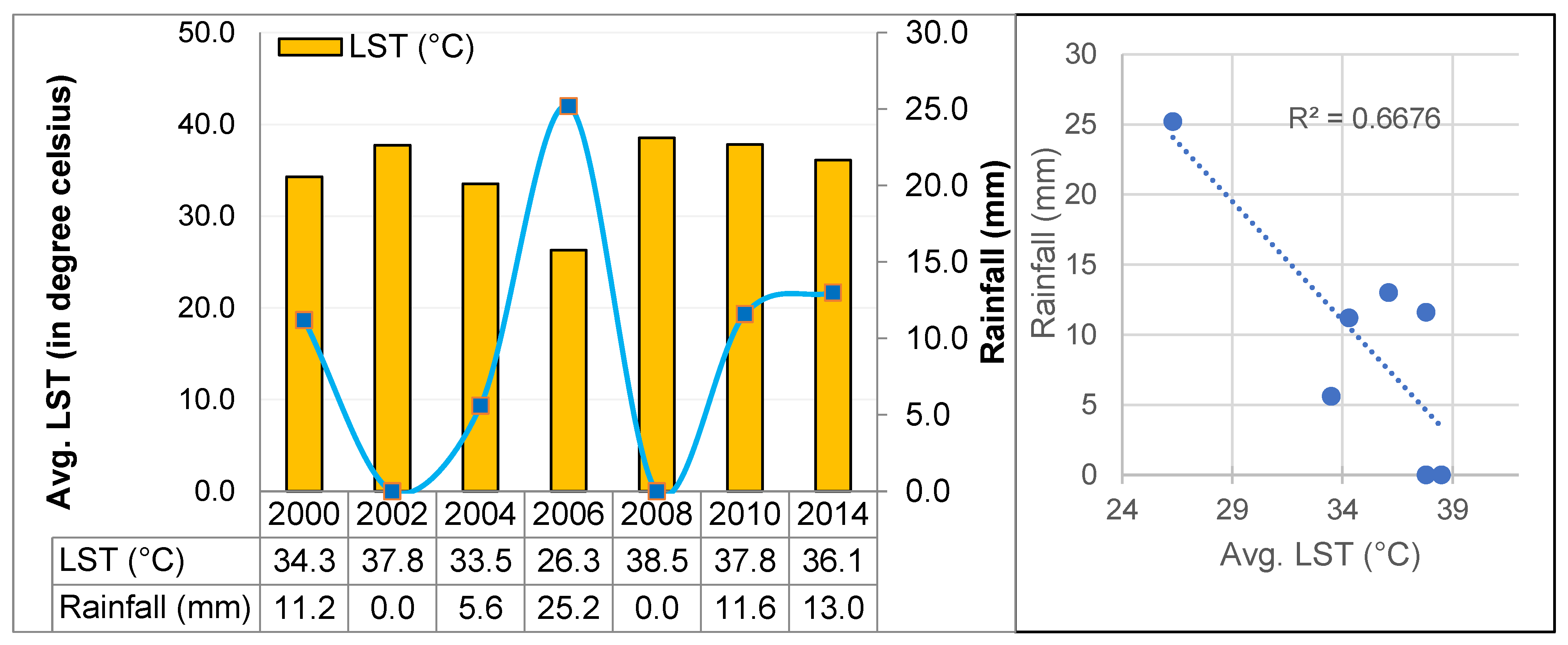
A total of 100 random sample points were generated over different land-use/land-cover regions, which remained unchanged from 2000 to 2014, to deduce the LST dynamics on varied LULC. Although the LST had almost increased all the observation years, the LST is influenced by rainfall, as due to rainfall, the moisture content of the upper layer of soil increases, which increases the thermal inertia of wet soil and controls the surface temperature. In general, there is an episodic increase and decrease in average LST with an overall increase (1.8 °C; 5.23%) in surface temperature from 2000 to 2014 (

Table 7. Average land surface temperature from 2000 to 2014 (May month).

LULC Features	2000	2002	2004	2006	2008	2010	2014	Avg. 2000–2014
Bare rock	39	42	37	28	43	42	39	38.6
Fallow land	37	40	35	25	42	39	36	36.3
Built-up (airport)	38	40	36	29	43	42	41	38.4
Built-up (high density)	37	40	36	27	39	40	38	36.7
Built-up (industrial)	40	43	38	31	43	43	42	40.0
Built-up (low density)	35	38	34	26	38	39	37	35.3
Built-up (railway)	40	42	37	28	44	40	38	38.4
Vegetation	28	33	31	24	35	34	33	31.1
Water body	25	29	26	22	29	30	29	27.1
Water body (waste)	25	30	26	23	29	31	29	27.6
Average	34.4	37.7	33.6	26.3	38.5	38	36.2	34.96

). The average surface temperature was 34.4 °C in 2000, which increased to 37.7 °C in 2002, and later significantly decreased to 33.6 °C and 26.3 °C in 2004 and 2006, respectively. It later increased to 38.5 °C in 2008 and slightly decreased to 38.0 °C in 2010 and later significantly decreased to 36.2 °C in 2014. The significant decrease in 2006 is attributed to the recent rainfall occurrence (cumulative 25 mm) during the last 7 days from the satellite data acquisition. The LST estimated on varied land use exhibited that the maximum LST was observed on bare rock (min: 28 °C and max: 43 °C), fallow land (min: 25 and max: 42 °C), and industrial built-up area (min: 31 °C and max: 43 °C), with average LST of 35 °C during 2000–14 (Table 7 and Figure 9a,b). The high-density built-up area (min: 27 °C and max: 40 °C) had an average LST of 32 °C followed by vegetation (min: 24 °C and max: 34 °C) and water body (min: 22 °C and max: 30 °C), which exhibited low LST with an average of 31 °C and 25 °C from 2000 to 2014.

3.7. Influence of Rainfall on LST

The average LST was correlated with the cumulative rainfall of the last seven days from the date of satellite data acquisition to analyze the influence of rainfall patterns on the LST in the Ranchi region. The study shows a significant negative correlation (R² = 0.66) between cumulative rainfall and average LST (Figure 10). The maximum cumulative rainfall was 25.2 mm (2006), followed by 13.0 mm (2014), 11.6 mm (2010), 11.2 mm (2000), and 5.6 mm (2004), wherein the LST was 26.3 °C, 36.1 °C, 37.8 °C, 34.3 °C, and 33.5 °C, respectively. The cumulative rainfall was absent/null during the years 2002 and 2008, when LST was 37.8 °C and 38.5 °C, respectively. During the rain-fed years (2000, 2004, 2006, 2010, 2014), the moisture content in the surface/soil contributes to minimizing the heat intensity by increasing the thermal inertia of the wet surface/soil. However, the LST was higher in the years of low or null. The increasing trend of erratic rainfall patterns in RUA reflects the low intensity of rainfall and loss of heat sink zones in contrast to the increasingly impervious surface as a contributing factor for higher LST [53]. The steady and continuous increase in temperature and decrease in rainfall provide an insight into the warming up of the eastern plateau region, highlighting the severe impact of anthropogenic activities [6,67]. The spatiotemporal built-up growth in the urban and peri-urban regions of the city highly influences the rainfall pattern through the development of UHI, unstable monsoon environment, etc. [68].

3.8. Influence of Altitudinal Variations on LST

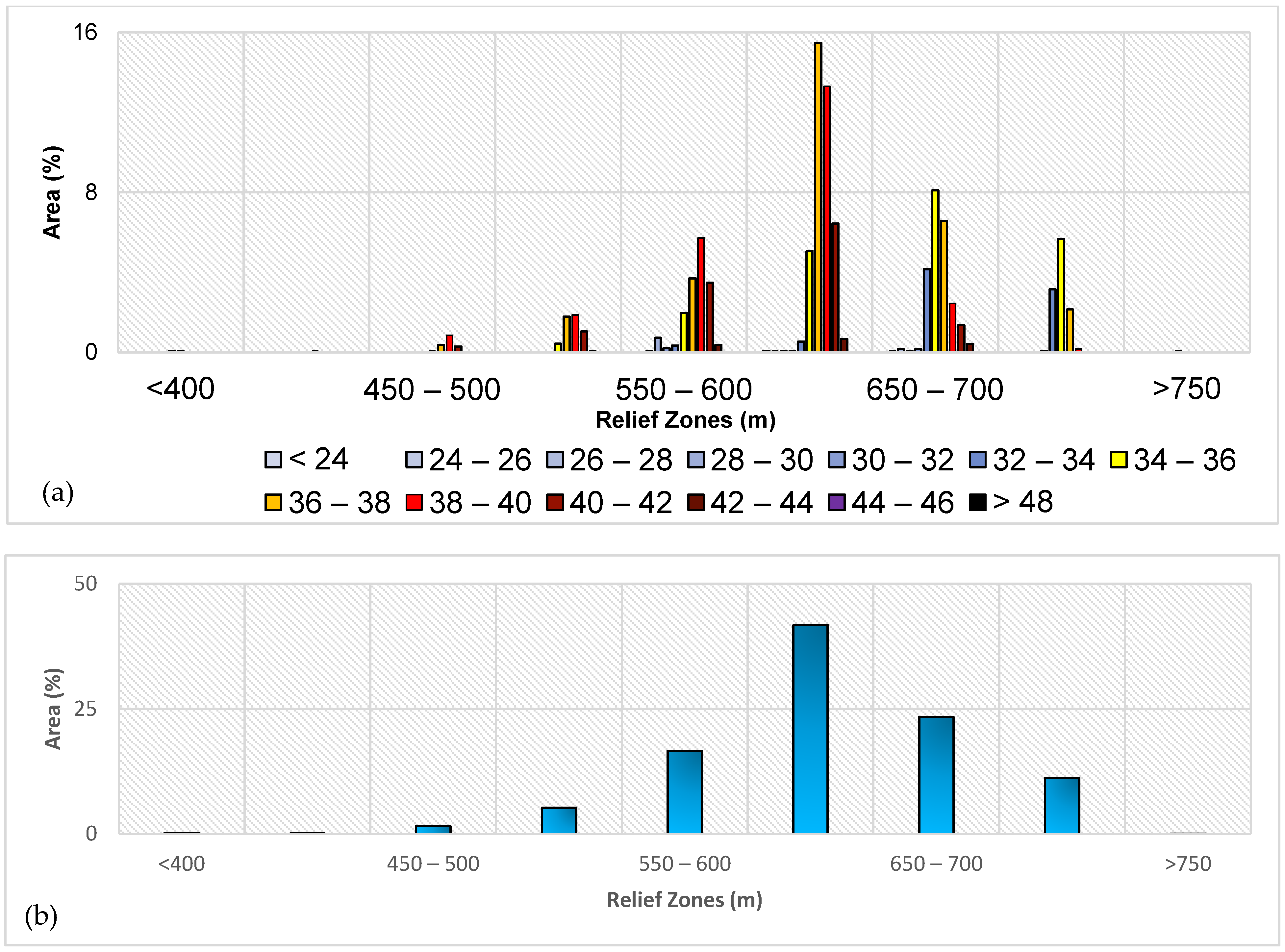
The CARTOSAT-I-based DEM (30 m) was used to analyze the potential correlation between LST (2014) and the relief zone in Ranchi. The study shows that the majority (41%) of RUA lies within a 600–650 m relief zone and is primarily comprised of built-up area and rock outcrops in the central and southeastern parts, wherein the LST ranges from 36 °C to 42 °C, primarily 36 °C to 40 °C (28.78% area; Figure 11 and Figure 12). The 650–700 m relief zone covers 23.45% of the area, wherein the majority of the area has 34 °C to 42 °C LST, primarily 34 °C to 38 °C (14.6% area). The relief zone 550–600 m covers 16.61% of the area in the central, north, and southern parts, wherein LST ranges from 32 °C to 42 °C, primarily 38–40 °C (5.72% area). The higher relief zone (>700 m) covers 11.3% of the area, with 34 °C to 38 °C LST, whereas the lower relief zones (<550 m) covering 6.9% of the area, are located in the eastern and southeastern parts, and have 36 °C to 40 °C LST.

4. Discussion

The present study highlights that Ranchi observed a comparatively lower temperature than its peri-urban regions due to the existence of barren and rock outcrops. Though the LST increased on all types of land surfaces within the urban area of Ranchi, it appears cooler than that of its peri-urban region, representing the dominance of exposed rocky surfaces of plateau origin, providing a good ease of living environment in Ranchi. In line with the same, a previous study reported the alteration in the local and regional climate due to the increasing annual per capita land consumption (361.50%), the annual per capita loss of heat sink zones (96.3% during 1927–2010), and the high influx of vehicles (563% from 1997 to 2010) [53]. Moreover, a high rise in ambient temperature was prevalent in the Ranchi urban area (by 4–6 °C) compared to its rural environment [56]. The state CNT Act has restricted the frequent transfer of tribal land to non-tribal communities, indirectly retaining the natural landscapes within the Ranchi city region, which play a vital role in heat sinking and regulation of land surface temperature. The development of green infrastructure and avenue plantations, the promotion of compact and sustainable urban development, the establishment of regulations and guidelines for land-use change, low-carbon technologies and practices, the promotion of energy-efficient buildings, and the use of renewable energy sources are some of the key measures to mitigate urban heat islands in the key areas of UHI hotspots [41,69]. Tree plantation, especially local climate-resilient native species [70], green roofing, use of light-colored concrete and white roofs [71], cool paint on the top floor, and roof ventilation [72], coupled with the implementation/sensitization of heat-reduction policies and rules, can be efficient measures to mitigate the increasing impact of UHI on the changing climatic conditions in urban and peri-urban regions. Governments can provide incentives or regulations to encourage the use of cool roofs in new and existing buildings [41]. The seasonal variability of LST using higher-resolution satellite data can provide a better understanding of inward-wise LST estimation and risk assessment due to the discomfort created by heat islands. Future work is recommended to simulate urban heat sink zones using modeling to derive the proper heat sink zone in an urban environment with hourly land skin temperature and air temperature. The increase in LST may be attributed to an increase in global skin temperature and air temperature [73], rapid land transformation to the impervious surface, deforestation, etc. Recurrent soil erosion induced an increasing concentration of suspended solids in the water and the dumping of non-treated industrial-municipal wastewater containing harmful effluents into the reservoir, leading to a decrease in oxygen demands and, ultimately, an increase in the surface water temperature. The degradation of vegetation coverage, its health, canopy depth, and soil wetness, particularly in the urban region due to the rapid urbanization process as well as pollution, accelerates the UHI phenomenon.

At the time of image acquisition, the city observed a few spots with high LST associated with high-density built-up land, airstrips, etc., which were characterized by very low or no vegetation cover. In contrast, the peri-urban area in the north and southeast portions observed major patches with high LST associated with bare land surfaces, which were characterized by negligible vegetation cover. In western parts, the heat island was formed on the western side, dominated by a rock outcrop and built-up land surrounded by heat sink zones of rural vegetative patches.

The caveat of the studies lies with the issues in the thermal channels of Landsat 5 and Landsat 7, which are used to capture thermal infrared data. The thermal channels are sensitive to changes in the detectors used to record the data, which can result in errors or anomalies in thermal imagery [74]. Moreover, the datasets acquired by the sensor are used for thermal characteristics of land surfaces and UHI estimation following the data documentation and guidance given by the USGS and NASA that assist in correctly handling thermal band errors in Landsat 5 and 7 imageries [75]. The use of numerical modeling to estimate critical issues such as pollution and erratic changes in climatic conditions aggravating the development of the UHI effect is very limited to Indian cities [76]. Most of the UHI studies are primarily based on one-time analysis considering daytime and only the summer season due to a lack of data availability, but the diurnal and seasonal variation of LST on urban landscapes requires incorporating advanced models and algorithms for better evaluation in the future [77]. LST estimation from 2000 to 2024 in the present study is attributed to the objective of assessing the changes in the thermal characteristics of urban and peri-urban regions after the reorganization of Ranchi as a state capital in 2000.

Future recommendations include: (a) an integrated urban planning approach with the availability of blue–green infrastructure to reduce the impact of UHI with reference to the level of urbanization and the development of heat sink zones for a healthy and sustainable environment; (b) energy-efficient construction practices such as promoting green roofs and walls, building codes, using permeable pavements, etc.; (c) developing policies and frameworks for the public awareness of water conservation practices; and (d) promoting a city-centric framework that ensures solutions that are locally appropriate and sustainable in the long term.

5. Conclusions

The study showed a rapid rise in built-up land (135% growth; 47.65 sq. km) from 2000 to 2014, causing irreversible loss primarily to vegetation (−6.8%), rock outcrops (−44.16%), and other (0.81%) land use/cover. Spatiotemporal LST variability exhibited an increase in area under the high-temperature zone (>38 °C) as compared to the moderate (30 °C to 38 °C) and low-temperature (<30 °C) zones during the period (2000–2014). Although the LST was distinctively escalating in all LULCs during the summer (May) from 2000 to 2014, large parts of the urban area were mostly observed to be less warm than peri-urban regions. The study demonstrated that the development of urban heat sink zones in urban areas is associated with the existence of vegetation and waterbodies spread throughout the city and UHIs driven by the large clusters of built-up surfaces. Within urban build-up, major heat islands formed over the densely built-up area, fallow land (bare soil), and rock outcrops. The study illustrated a rise in the surface temperature of all the LULCs during the summer (May; 2000–2014) with an increase in the average temperature of about 1.80 °C while considering pure summer weeks with null/least influence of pre-monsoon showers. The highest surface temperature was observed over the bare rock (min/max: 28–43 °C), followed by fallow land (min/max: 25–42 °C), industrial built-up area (min/max: 31–43 °C), and high-density built-up area (min/max: 27–40 °C), while the relatively lower temperature was observed in vegetation (min/max: 24–34 °C) and water bodies (min/max: 22–30 °C). The results highlighted that low vegetation cover plays an important role in the rise in daytime LST in peri-urban areas. The study provides insight into the local and regional microclimatic conditions of urban landscapes. It also offers insight into the exacerbation of the severe effects of climate change, the improvement of quality of life, and the development of adaptation strategies to supplement informed decisions and policy frameworks for urban planning.