
Hydrochemical Indicator Analysis of Seawater Intrusion into Coastal Aquifers of Semiarid Areas

 , , and
Abstract
1. Introduction

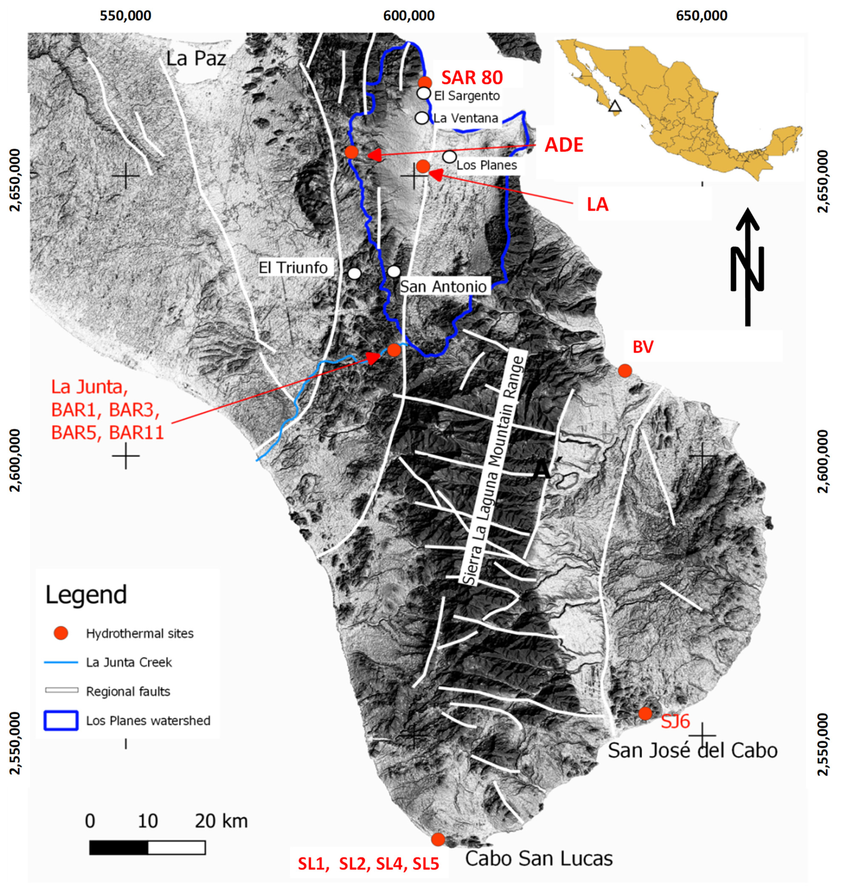
2. Regional Setting
2.1. Climate
2.2. Geological Setting
2.3. Hydrogeological Framework
2.4. Geothermal Framework
2.5. Agriculture and Industrial Activities
3. Materials and Methods
3.1. Water Samples Documented in Former Studies (for Water Quality and Seawater Intrusion Estimation)
3.2. Recognizing Seawater Intrusion by Different Methods
3.2.1. Classification of Seawater Freshening
3.2.2. Calculation of the Seawater Fraction and Mixing Index
Seawater Fraction
Saltwater Mixing Index (SMI)
3.2.3. Hydrochemical Facies Evolution Diagram
3.3. Thermal Water
4. Results and Discussion
4.1. Water Quality
4.2. Groundwater Types
4.3. Calculation of the Seawater Fraction Based on Ion Ratios
4.4. Salinity Origin after the Hydrochemical Facies Evolution Diagram
5. Geothermal Water
6. Conclusions
Supplementary Materials
Author Contributions
Funding
Informed Consent Statement
Data Availability Statement
Conflicts of Interest
References
- Polemio, M.; Walraevens, K. Recent research results on groundwater resources and saltwater intrusion in a changing environment. Water 2019, 11, 1118. [Google Scholar] [CrossRef]
- Ferguson, G.; Gleeson, T. Vulnerability of coastal aquifers to groundwater use and climate change. Nat. Clim. Chang. 2012, 2, 342–345. [Google Scholar] [CrossRef]
- Werner, A.D.; Bakker, M.; Post, V.E.A.; Vandenbohede, A.; Lu, C.; Ataie-Ashtiani, B.; Simmons, C.T.; Barry, D.A. Seawater intrusion processes, investigation and management: Recent advances and futures challenges. Adv. Water Resour. 2013, 51, 3–26. [Google Scholar] [CrossRef]
- Tran, D.A.; Tsujimura, M.; Pham, H.V.; Nguyen, T.V.; Ho, L.H.; Vo, P.L.; Ha, K.Q.; Dang, T.D.; Vinh, D.V.; Doan, Q.-V. Intensified salinity intrusion in coastal aquifers due to groundwater overextraction: A case study in the Mekong Delta, Vietnam. Environ. Sci. Pollut. Res. 2022, 29, 8996–9010. [Google Scholar] [CrossRef]
- Mahlknecht, J.; Merchán, D.; Rosner, M.; Meixner, A.; Ledesma-Ruis, R. Assessing seawater intrusion in an arid coastal aquifer under high anthropogenic influence using major constituents, Sr and B isotopes in groundwater. Sci. Total Environ. 2017, 587, 282–295. [Google Scholar] [CrossRef]
- Comisión Nacional de Agua. Estadísticas del Agua en México. 2018. Available online: http://sina.conagua.gob.mx/publicaciones/EAM_2018.pdf (accessed on 16 January 2023).
- Sistema Nacional de Información del Agua (SNIA-CONAGUA). Tablas de Sobreexplotación y Salinización de Acuíferos en México para el Año 2021. 2021. Available online: http://sina.conagua.gob.mx/sina/tema.php?tema=acuiferos (accessed on 9 January 2023).
- Fichera, M.M. Numerical Modeling and Hydrochemical Analysis of the Current and Future State of Seawater Intrusion in the Todos Santos Aquifer, Mexico. Ph.D. Thesis, Colorado State University, Fort Collins, CO, USA, 2019. Available online: https://mountainscholar.org/bitstream/handle/10217/195327/Fichera_colostate_0053N_15368.pdf (accessed on 16 January 2023).
- Chávez-López, S.; Brito-Castillo, L. Calidad del agua subterránea en la Reserva de La Biosfera de El Vizcaino BCS, México. Rev. Latinoam. Recur. Nat. 2010, 6, 7–20. [Google Scholar]
- González-Abraham, A.; Fagundo-Castillo, J.R.; Carillo-Rivera, J.J.; Rodríguez-Estrella, R. Geoquímica de los sistemas de flujo de agua subterránea en rocas sedimentarias y vulcanogénicas de Loreto, BCS, México. Bol. Soc. Geol. Mex. 2012, 6, 319–333. [Google Scholar] [CrossRef]
- Cardona, A.; Carrillo-Rivera, J.J.; Huizar-Alvarez, R.; Graniel-Castro, E. Salinization in coastal aquifers of arid zones: An example from Santo Domingo, Baja California Sur, Mexico. Environ. Geol. 2004, 45, 350–366. [Google Scholar] [CrossRef]
- Wurl, J.; Gámez, A.E.; Ivanova-Boncheva, A.; Imaz-Lamadrid, M.A.; Hernández-Morales, P. Socio-hydrological resilience of an arid aquifer system, subject to changing climate and inadequate agricultural management: A case study from the Valle of Santo Domingo, México. J. Hydrol. 2018, 559, 486–498. [Google Scholar] [CrossRef]
- Arango-Galván, C.; Prol-Ledesma, R.M.; Torres-Vera, M.A. Geothermal prospects in the Baja California Peninsula. Geothermics 2015, 55, 39–57. [Google Scholar] [CrossRef]
- Comisión Nacional de Agua (CNA). Determinación de la Disponibilidad de Agua en el Acuífero (0323) Los Planes, Estado de Baja California Sur. 2003. Available online: http://defiendelasierra.org/wp-content/uploads/Estudio-CNA-Intrusion-Salina-y-Metales-Pesados-Los-Planes.pdf (accessed on 16 January 2023).
- Briseño Arellano, 2014 Evaluación de la Evolución Hidrogeoquímica del Agua Subterránea en La Cuenca San Juan de Los Planes, Baja California Sur 2014 Tesis Lic. UNAM. Available online: https://repositorio.unam.mx/covers/133713/0/300.png (accessed on 16 January 2023).
- Del Rosal Pardo, A. Recarga Natural en la Cuenca de San Juan de los Planes, Baja California Sur, México. Bachelor’s Thesis, Universidad Autónoma de Baja California Sur, La Paz, México, 2003. [Google Scholar]
- Busch, M.M.; Arrowsmith, J.R.; Umhoefer, P.J.; Coyan, J.A.; Maloney, S.J.; Gutiérrez, G.M. Geometry and evolution of rift-margin, normal-fault–bounded basins from gravity and geology, La Paz–Los Cabos region, Baja California Sur, Mexico. Lithosphere 2011, 3, 110–127. [Google Scholar] [CrossRef]
- Coyan, M.M.; Arrowsmith, J.R.; Umhoefer, P.; Coyan, J.; Kent, G.; Driscoll, N.; Gutíerrez, G.M. Geometry and Quaternary slip behavior of the San Juan de los Planes and Saltito fault zones, Baja California Sur, Mexico: Characterization of rift-margin normal faults. Geosphere 2013, 9, 426–443. [Google Scholar] [CrossRef]
- NASA. NASA Shuttle Radar Topography Mission (SRTM) Version 3.0 (SRTM Plus) Product Release. Land Process Distributed Active Archive Center, National Aeronautics and Space Administration. 2013. Available online: https://lpdaac.usgs.gov/news/nasa-shuttle-radar-topography-mission-srtm-version-30-srtm-plus-product-release/ (accessed on 28 October 2021).
- Aranda-Gómez, J.J.; Pérez-Venzor, J.A. Estratigrafía del complejo cristalino de la región de Todos Santos, estado de Baja California Sur. Revista 1989, 8, 149–170. [Google Scholar]
- Fletcher, J.M.; Kohn, B.P.; Foster, D.A.; Gleadow, A.J.W. Heterogeneous Neogene cooling and exhumation of the Los Cabos block, southern Baja California: Evidence from fission-track thermochronology. Geology 2000, 28, 107–110. [Google Scholar] [CrossRef]
- Schaaf, P.; Böhnel, H.; Pérez-Venzor, J.A. Pre-Miocene palaeogeography of the Los Cabos block, Baja California Sur: Geochronological and palaeomagnetic constraints. Tectonophysics 2000, 318, 53–69. [Google Scholar] [CrossRef]
- CONAGUA Comisión Nacional de Agua. Determinación de la Disponibilidad de Agua en el Acuífero (0323) Los Planes, Estado de Baja California Sur. 2020. Available online: https://sigagis.conagua.gob.mx/gas1/Edos_Acuiferos_18/BajaCaliforniaSur/DR_0323.pdf (accessed on 16 January 2023).
- Wurl, J.; Martínez Gutiérrez, G. El efecto de ciclones tropicales sobre el clima en la cuenca de Santiago, Baja California Sur, México. In Proceedings of the III Simposio Internacional en Ingeniería y Ciencias para la Sustentabilidad Ambiental y Semana del Ambiente, Mexico City, Mexico, 5–6 June 2006. [Google Scholar]
- Dominguez, C.; Magaña, V. The Role of Tropical Cyclones in Precipitation over the Tropical and Subtropical North America. Front. Earth Sci. 2018, 6, 19. [Google Scholar] [CrossRef]
- Gutiérrez Caminero, L. Isótopos de Pb como Trazadores de Fuentes de Metales y Metaloides en el Distrito Minero San Antonio-El Triunfo, Baja California Sur. Master’s Thesis, Centro de Investigación Científica y de Educación Superior de Ensenada, Ensenada, Mexico, 2013. [Google Scholar]
- Aranda-Gómez, J.J.; Pérez-Venzor, J.A. Excursión Geológica al Complejo Migmatítico de la Sierra de La Gata, BCS III Reunión Internacional Sobre la Geología de la Península de Baja California; Sociedad Geológica Peninsular en la Universidad Autónoma de Baja California Sur: La Paz, Mexico, 1995; pp. 17–27. [Google Scholar]
- CNA (Comisión Nacional del Agua), Gerencia de Aguas Subterránea. 1997; Estudio Hidrogeológico y Simulación Hidrodinámica del Acuífero del Valle de San Juan de los Planes, B.C.S. Final report; Dirección Local en Baja California Sur, unpublished. [Google Scholar]
- Técnicas Modernas de la Ingeniería (TMI), S.A. 1977; Informe final del Estudio Geohidrológico del valle de San Juan de los Planes, en el estado de Baja California Sur, para la Subdirección de Geohidrología y de Zonas Áridas SARH, unpublished. [Google Scholar]
- Prol-Ledesma, R.M.; Canet, C.; Torres-Vera, M.A.; Forrest, M.J.; Armienta, M.A. Vent fluid chemistry in Bahía Concepción coastal submarine hydrothermal system. J. Volcanol. Geotherm. Res. 2004, 137, 311–328. [Google Scholar] [CrossRef]
- Prol-Ledesma, R.M.; Dando, P.R.; De Ronde, C.E.J. Special issue on shallow-water hydrothermal venting. Chem. Geol. 2005, 224, 1–4. [Google Scholar] [CrossRef]
- Carrillo, A. Environmental Geochemistry of the San Antonio-El Triunfo Mining Area, Southernmost Baja California Peninsula Mexico. Ph.D. Thesis, University of Wyoming, Laramie, WY, USA, 1996. [Google Scholar]
- COREMI (Consejo de Recursos Minerales). Monografía Geológico-Minera del Estado de Baja California Sur; Secretaría de Comercio y Fomento Industrial: Ciudad Juárez, México, 1999. [Google Scholar]
- Carrillo-Chavez, A.; Drever, J.I.; Martinez, M. Arsenic content and groundwater geochemistry of the San Antonio-El Triunfo, Carrizal and Los Planes aquifers in southernmost Baja California, Mexico. Environ. Geol. 2000, 39, 1295–1303. [Google Scholar] [CrossRef]
- Naranjo-Pulido, A.; Romero-Schmidt, H.; Mendez-Rodriguez, L.; Acosta-Vargas, B.; Ortega-Rubio, A. Soil arsenic contamination in the Cape Region, BCS, Mexico. J. Environ. Biol. 2002, 23, 347–352. [Google Scholar] [PubMed]
- Carrillo, A.; Drever, J.I. Environmental assessment of the potential for arsenic leaching into groundwater from mine wastes in Baja California Sur, Mexico. Geofísica Int. 1998, 37, 35–39. [Google Scholar] [CrossRef]
- Volke-Sepúlveda, T.; Solórzano-Ochoa, G.; Rosas-Domínguez, A.; Izumikawa, I.; Encarnación-Aguilar, G.; Velasco-Trejo, J.A.; Flores Martínez, S. Informe Final, Remediacion de Sitios Contaminados por Metales Provenientes de Jales Mineros en Los Distritos de El Triunfo-San Antonio y Santa Rosalía, Baja California Sur, Mexico, 2003; 37p. Available online: http://defiendelasierra.org/wp-content/uploads/Estudio-de-Remediaci%C3%B3n-El-Triunfo-y-San-Antonio-2003.pdf (accessed on 16 January 2023).
- DVWK-Regeln Zur Wasserwirtschaft, H. Entnahme und Untersuchungsumfang von Grundwasserproben. In DK 556.32.001.5 Grundwasseruntersuchung, DK 543.3.053 Probenahme. DVWK-Regeln zur Wasserwirtschaft 128, 36; Deutscher Verband für Wasserwirtschaft und Kulturbau e.V.: Hamburg/Berlin, Germany, 1992. (In German) [Google Scholar]
- Wurl, J.; Mendez-Rodriguez, L.; Acosta-Vargas, B. Arsenic content in groundwater from the southern part of the San Antonio-El Triunfo mining district, Baja California Sur, Mexico. J. Hydrol. 2014, 518, 447–459. [Google Scholar] [CrossRef]
- U.S. Environmental Protection Agency. Method 6020A—Inductively Coupled Plasma Mass Spectrometry; Revision 1; U.S. Environmental Protection Agency: Washington, DC, USA, 2007. [Google Scholar]
- Appelo, C.A.J.; Postma, D. Geochemistry, Groundwater and Pollution; A.A. Balkema: Rotterdam, The Netherlands, 1995. [Google Scholar]
- Giménez-Forcada, E. Dynamic of Seawater Interface using Hydrochemical Facies Evolution Diagram (HFE-D). Groundwater 2010, 48, 212–216. [Google Scholar] [CrossRef]
- Giménez-Forcada, E. Use of the Hydrochemical Facies Diagram (HFE-D) for the evaluation of salinization by seawater intrusion in the coastal Oropesa Plain: Comparative analysis with the coastal Vinaroz Plain, Spain. HydroResearch 2019, 2, 76–84. [Google Scholar] [CrossRef]
- Ibrahim Hussein, H.A.; Ricka, A.; Kuchovsky, T.; El Osta, M.M. Groundwater hydrochemistry and origin in the south-eastern part of Wadi El Natrun, Egypt. Arab. J. Geosci. 2017, 10, 170. [Google Scholar] [CrossRef]
- Klassen, J.; Allen, D.M.; Kirste, D. Chemical Indicators of Salt Water Intrusion for the Gulf Islands, British Columbia; Department of Earth Sciences, Simon Fraser University: Burnaby, BC, Canada, 2014; 43p. [Google Scholar]
- Carreira, P.M.; Marques, J.M.; Nunes, D. Source of groundwater salinity in coastline aquifers based on environmental isotopes (Portugal): Natural vs. human interference. A review and reinterpretation. Appl. Geochem. 2014, 41, 163–175. [Google Scholar] [CrossRef]
- Kelly, F. Seawater Intrusion Topic Paper; Island Country Health Department: Coupeville, WA, USA, 2005. [Google Scholar]
- Anderson, W.P., Jr. Aquifer salinization from storm overwash. J. Coast. Res. 2002, 18, 413–420. [Google Scholar]
- White, W.M. Geochemistry; John Wiley & Sons: Hoboken, NJ, USA, 2020. [Google Scholar]
- Park, C.H.; Aral, M.M. Saltwater intrusion hydrodynamics in a tidal aquifer. J. Hydrol. Eng. 2008, 13, 863–872. [Google Scholar] [CrossRef]
- Gupta, S.K.; Gupta, I.C. Drinking Water Quality Assessment and Management; Scientific Publishers: Jodhpur, India, 2020. [Google Scholar]
- Edet, A. Hydrogeology and groundwater evaluation of a shallow coastal aquifer, southern AkwaIbom State (Nigeria). Appl. Water Sci. 2017, 7, 2397–2412. [Google Scholar] [CrossRef]
- Van Le, T.T.; Lertsirivorakul, R.; Bui, T.V.; Schulmeister, M.K. An application of HFE-D for evaluating seawater intrusion in coastal aquifers of Southern Vietnam. Groundwater 2020, 58, 1012–1022. [Google Scholar] [CrossRef]
- Sajil Kumar, P.J. Deciphering the groundwater–saline water interaction in a complex coastal aquifer in South India using statistical and hydrochemical mixing models. Model. Earth Syst. Environ. 2016, 2, 1–11. [Google Scholar] [CrossRef]
- Giggenbach, W.F.; Goguel, R.L. Collection and Analysis of Geothermal and Volcanic Water and Gas Discharges; Report No. CD 2401; Department of Scientific and Industrial Research, Chemistry Division: Petone, New Zealand, 1989. [Google Scholar]
- López-Sánchez, A.; Báncora-Alsina, C.; Prol-Ledesma, R.M.; Hiriart, G. A new geotermal resource in Los Cabos, Baja California Sur, Mexico. In Proceedings of the 28th New Zealand Geothermal Workshop, Auckland, New Zealand, 15–17 November 2006. [Google Scholar]
- Hernández-Morales, P.; Wurl, J. Hydrogeochemical characterization of the thermal springs in northeastern of Los Cabos Block, Baja California Sur, Mexico. Environ. Sci. Pollut. Res. 2016, 24, 13184–13202. [Google Scholar] [CrossRef]
- Stigter, T.Y.; Carvalho Dill, A.M.M.; Ribeiro, L.; Reis, E. Impact of the shift from groundwater to surface water irrigation on aquifer dynamics and hydrochemistry in a semi-arid region in the south of Portugal. Agric. Water Manag. 2006, 85, 121–132. [Google Scholar] [CrossRef]
- Portugal, E.; Birkle, P.; Barragán, R.M.; Arellano, V.M.; Tello, E.; Tello, M. Hydrochemical-isotopic and hydrogeological conceptual model of the Las Tres Vírgenes geothermal field, Baja California Sur, México. J. Vulcanol. Geotherm. Res. 2000, 101, 223–244. [Google Scholar] [CrossRef]
- Canet, C.; Prol-Ledesma, R.M.; Proenza, J.A.; Rubio-Ramos, M.A.; Forrest, M.J.; Torres-Vera, M.A.; Rodríguez-Díaz, A.A. Mn–Ba–Hg mineralization at shallow submarine hydrothermal vents in Bahía Concepción, Baja California Sur, Mexico. Chem. Geol. 2005, 224, 96–112. [Google Scholar] [CrossRef]
- Villanueva-Estrada, R.E.; Prol-Ledesma, R.M.; Torres-Alvarado, I.S.; Canet, C. Geochemical modeling of a Shallow Submarine Hydrothermal System at Bahía Concepción, Baja California Sur, México. In Proceedings of the World Geothermal Congress, Antalya, Turkey, 24–29 April 2005. [Google Scholar]
- Verma, S.P.; Santoyo, E. New improved equations for Na/K, Na/Li and SiO2 geothermometers by outlier detection and rejection. J. Volcanol. Geotherm. Res. 1997, 79, 9–24. [Google Scholar] [CrossRef]
- Vengosh, A.; Gill, J.; Davisson, M.L.; Hudson, G.B. A multi-isotope (B, Sr, O, H, and C) and age dating (3H–3He and 14C) study of groundwater from Salinas Valley, California: Hydrochemistry, dynamics, and contamination processes. Water Resour. Res. 2002, 38, 9-1-9-17. [Google Scholar] [CrossRef]
- Nordstrom, D.K.; Plummer, L.N.; Wigley, T.M.L.; Wolery, T.J.; Ball, J.W.; Jenne, E.A.; Bassett, R.L.; Crerar, D.A.; Florence, T.M.; Fritz, B. A Comparison of Computerized Chemical Models for Equilibrium Calculations in Aqueous Systems. In Chemical Modeling in Aqueous Systems; American Chemical Society: Washington, DC, USA, 1979; pp. 857–892. [Google Scholar] [CrossRef]
- Powell, T.; Cumming, W. Spreadsheets for geothermal water and gas geochemistry. In Proceedings of the Thirty-Fifth Workshop on Geothermal Reservoir Engineering, Stanford, CA, USA, 1–3 February 2010. 10p. [Google Scholar]
- Goosen, M.; Mahmoudi, H.; Ghaffour, N. Water desalination using geothermal energy. Energies 2010, 3, 1423–1442. [Google Scholar] [CrossRef]


| Year | Extraction Volume Million m3/Year | Recharge Million m3/Year | Deficit Million m3/Year |
|---|---|---|---|
| 2003 | 12.29 | 9.89 | −2.40 |
| 2007 | 12.29 | 8.40 | −3.89 |
| 2013 | 12.29 | 8.26 | −4.03 |
| 2015 | 12.29 | 8.40 | −3.89 |
| 2020 | 13.10 | 8.40 | −4.70 |
| Season | Crop | Irrigation System | Irrigated Surface (ha) | Net Volume Used (m3) | Irrigation Return (m3/Year) |
|---|---|---|---|---|---|
| Winter | Chile | Drip | 160 | 1,200,000 | 48,000 |
| Chile | Flood gates | 340 | 2,550,000 | 484,500 | |
| Tomato | Drip | 60 | 462,000 | 18,480 | |
| Corn | Irrigation channel | 65 | 286,000 | 111,540 | |
| Cotton | Flood gates | 30 | 210,000 | 39,900 | |
| Cucumber | Drip | 50 | 200,000 | 8000 | |
| Beans | Aspersion irrigation | 50 | 190,000 | 26,600 | |
| Subtotal | 755 | 5,098,000 | 737,020 | ||
| Summer | Corn | Irrigation channel | 135 | 594,000 | 231,660 |
| Subtotal | 135 | 594,000 | 231,660 | ||
| Perennial | Alfalfa | Aspersion irrigation | 50 | 600,000 | 84,000 |
| Fruit trees | Aspersion irrigation | 15 | 180,000 | 25,200 | |
| Subtotal | 65 | 780,000 | 109,200 | ||
| Total | 955 | 6,472,000 | 1,077,880 |
| Campaign | Temp | pH | Ca2+ | Mg2+ | Na+ | K+ | HCO3– | SO42– | Cl– | TDS | |
|---|---|---|---|---|---|---|---|---|---|---|---|
| °C | mg/L | mg/L | mg/L | mg/L | mg/L | mg/L | mg/L | mg/L | |||
| 2003 * | Minimum | 38.6 | 6.9 | 13.30 | 4.90 | 66.00 | 2.30 | 91.12 | 23.00 | 50.30 | 309 |
| 2003 * | Maximum | 32.0 | 8.2 | 172.40 | 78.80 | 550.00 | 19.60 | 257.28 | 375.00 | 893.40 | 2007 |
| 2003 * | Average. | 30.0 | 77.81 | 31.90 | 205.52 | 6.22 | 152.02 | 137.47 | 309.66 | 907 | |
| 2003 * | St. Dev. | 1.8 | 48.84 | 24.68 | 145.79 | 4.31 | 43.86 | 105.85 | 264.69 | 580 | |
| 2014–2016 ** | Minimum | 30.5 | 7.2 | 9.37 | 8.38 | 63.01 | 0.86 | 122.00 | 21.78 | 45.65 | 340 |
| 2014–2016 ** | Maximum | 37.8 | 8.5 | 213.62 | 176.93 | 1239.5 | 43.25 | 316.07 | 454.61 | 1917.4 | 4145 |
| 2014–2016 ** | Average. | 26.9 | 76.66 | 46.62 | 274.74 | 7.02 | 186.94 | 158.14 | 447.71 | 1190 | |
| 2014–2016 ** | St. Dev. | 2.35 | 57.51 | 43.65 | 269.87 | 9.52 | 47.68 | 150.93 | 456.44 | 916 | |
| Classification | 2003 | 2014–2016 |
|---|---|---|
| Intrusion | 7 | 8 |
| Conservative mixing | 6 | 5 |
| Slight conservative mixing | 3 | 2 |
| Slight freshening | 2 | 2 |
| Freshening | 1 | 2 |
| SUMA | 19 | 19 |
| Ref. | fsea % | fsea % | fsea % |
|---|---|---|---|
| 2003 | 2014–2016 | Difference | |
| 1 | 3.69 | 4.11 | 0.42 |
| 2 VEN | 4.21 | 9.39 | 5.18 |
| 3 BAJ | 0.49 | 0.97 | 0.48 |
| 4 | 0.09 | 0.09 | −0.00 |
| 5 | 1.11 | 3.04 | 1.93 |
| 6 | −0.03 | −0.03 | −0.00 |
| 7 | 0.01 | −0.08 | −0.09 |
| 8 | 0.47 | 0.24 | −0.23 |
| 9 | −0.03 | −0.01 | 0.02 |
| 10 | 0.43 | 0.67 | 0.23 |
| 11 | 0.29 | 0.26 | −0.03 |
| 12 | 1.67 | 1.23 | −0.44 |
| 13 | 1.76 | 1.61 | −0.15 |
| 14 | 1.05 | 0.80 | −0.24 |
| 15 | 3.64 | 2.63 | −1.01 |
| 16 | 1.73 | 4.17 | 2.44 |
| 17 | 1.27 | 1.87 | 0.60 |
| 18 | −0.05 | −0.02 | 0.03 |
| 19 | 0.49 | 0.87 | 0.38 |
| LA * | 3.1 | ||
| SAR * | 88.5 | ||
| P Sar * | 3.6 | ||
| ADE * | −0.2 |
| Site | 2003 | 2014–2016 | ||||
|---|---|---|---|---|---|---|
| No. | Phase | Facies | Phase | Facies | ||
| 1 | Intrus. | Na | Cl | Intrus. | Na | Cl |
| 2 VEN | Intrus. | Na | Cl | Intrus. | Na | Cl |
| 3 BAJ | Fresh. | Na | Cl | Fresh. | Na | Cl |
| 4 | Fresh. | Na | MixHCO3 | Fresh. | Na | HCO3 |
| 5 | Fresh. | Na | Cl | Intrus. | Na | Cl |
| 6 | Fresh. | Na | HCO3 | Fresh. | Na | HCO3 |
| 7 | Fresh. | MixNa | HCO3 | Fresh. | Na | HCO3 |
| 8 | Intrus. | MixNa | Cl | Fresh. | Na | MixHCO3 |
| 9 | Fresh. | Na | HCO3 | Fresh. | Na | HCO3 |
| 10 | Fresh. | Na | MixCl | Fresh. | Na | Cl |
| 11 | Fresh. | Na | MixCl | Fresh. | Na | MixCl |
| 12 | Intrus. | MixCa | Cl | Intrus. | MixNa | MixSO4 |
| 13 | Intrus. | Na | Cl | Intrus. | MixNa | MixCl |
| 14 | Intrus. | MixNa | Cl | Intrus. | MixNa | Cl |
| 15 | Intrus. | Na | Cl | Fresh. | Na | Cl |
| 16 | Intrus. | MixNa | Cl | Intrus. | MixNa | Cl |
| 17 | Intrus. | MixNa | Cl | Intrus. | MixNa | Cl |
| 18 | Fresh. | Na | HCO3 | Fresh. | Na | HCO3 |
| 19 | Fresh. | Na | Cl | Intrus. | Na | Cl |
| LA | Fresh. | Na | Cl | |||
| ADE | Intrus. | Ca | HCO3 | |||
| P Sar | Fresh. | Na | Cl | |||
| SAR 80 | Fresh. | Na | Cl | |||
| Site | Key | pH | Temperature (°C) | Redox (mV) | Electrical Conductivity (µS/cm) |
|---|---|---|---|---|---|
| Los Angeles | LA | 7.37 | 48.7 | −157.5 | 5500 |
| Agua Ademadas | ADE | 6.59 | 26.8 | −1163.1 | 120 |
| La Ventana | VEN | 7.09 | 32.3 | -- | 2480 |
| El Bajio | BAJ | 7.69 | 38.6 | −1139.8 | 960 |
| Pozo Sargento | P Sar | 7.91 | 29.0 | -- | 5990 |
| Sargento 80 °C | SAR 80 | 7.8 | 80.0 | -- | -- |
| La Junta Creek * | BAR 1 | 9.49 | 25.6 | −370.0 | 393 |
| La Junta Creek * | BAR 3 | 9.33 | 26.4 | −287.7 | 325 |
| La Junta Creek * | BAR 5 | 9.61 | 26.1 | −270.0 | 632 |
| La Junta Creek * | BAR 11 | 9.44 | 28.5 | −410.0 | 390 |
| Buenavista ** | BV | 8.04 | 41.3 | 36.1 | 773 |
| C. San Lucas 1 *** | SL1 | 6.9 | 25 | -- | 1700 |
| C. San Lucas 2 *** | SL2 | 6.4 | 22 | -- | 3530 |
| C. San Lucas 4 *** | SL4 | 5.6 | 42 | -- | 28,200 |
| C. San Lucas 5 *** | SL5 | 5.7 | 72 | -- | 49,600 |
| San Jose del Cabo. 6 *** | SJ6 | 7.3 | 36 | -- | 6750 |
| Seawater M7 **** | M7 | 7.8 | 25 | -- | -- |
| Sample | Na | K | Ca | Mg | B |
|---|---|---|---|---|---|
| LA | 460.6 | 15.0 | 68.6 | 8.9 | 1.1 |
| ADE | 29.9 | 0.5 | 40.0 | 6.2 | 0.1 |
| VEN | 550.0 | 19.6 | 105.6 | 67.6 | -- |
| BAJ | 146.0 | 4.7 | 36.7 | 15.1 | -- |
| P Sar | 554.5 | 9.2 | 60.8 | 30.7 | 1.0 |
| SAR 80 | 15,136.9 | 509.0 | 589.1 | 569.4 | 8.2 |
| Bar 1 * | 90.2 | 1.5 | 2.0 | 0.1 | 9.5 |
| Bar 3 * | 97.5 | 1.2 | 2.6 | 0.1 | 6.0 |
| Bar 5 * | 87.9 | 1.4 | 1.9 | 0.1 | 0.8 |
| Bar 11 * | 85.2 | 0.5 | 4.8 | 0.2 | 2.0 |
| BV ** | 152 | 4.31 | 5.2 | 0.63 | 0.3 |
| SL1 *** | 290.0 | 14.1 | 27.0 | 47.1 | -- |
| SL2 *** | 722.0 | 35.0 | 32.0 | 59.0 | -- |
| SL4 *** | 5070.0 | 283.0 | 1210.0 | 75.0 | -- |
| SL5 *** | 9820.0 | 631.0 | 2430.0 | 69.6 | -- |
| SJ6 *** | 1090.0 | 33.0 | 190.0 | 83.7 | -- |
| M7 **** | 11,176.0 | 487.0 | 392.0 | 1400.0 | -- |
| Sample | Cl | F | SO4 | HCO3 |
|---|---|---|---|---|
| LA | 674.0 | 0.1 | 85.4 | 200 |
| ADE | 21.0 | 0.1 | 3.4 | 195 |
| VEN | 893.4 | 0.1 | 187.5 | 205.7 |
| BAJ | 158.1 | 0.1 | 55.0 | 170.0 |
| P Sar | 769.0 | 0.1 | 149.0 | 300 |
| SAR 80 | 14,141.9 | 3.9 | 1670.6 | 100 |
| Bar 1 * | 58.3 | 1.8 | 56.3 | 70.3 |
| Bar 3 * | 88.6 | 3.2 | 33.6 | 75.8 |
| Bar 5 * | 53.0 | 0.6 | 48.6 | 237 |
| Bar 11 * | 36.5 | 2.3 | 40.8 | 59.7 |
| BV ** | 121.5 | 2.22 | 59 | 7.2 |
| SL1 *** | 1279 | 0.1 | 105 | 371.9 |
| SL2 *** | 1826 | 0.1 | 200 | 278.9 |
| SL4 *** | 9132 | 1.7 | 625 | 93.0 |
| SL5 *** | 15,708 | 6.9 | 650 | 93.0 |
| SJ6 *** | 2557 | 2.9 | 500 | 325.4 |
| M7 **** | 18,744 | 0.1 | 2554 | 97.6 |
| Sample | pH | Na | K | Ca | Mg | F | Cl | SO4 | HCO3 |
|---|---|---|---|---|---|---|---|---|---|
| 07 PLRC 41 | 5.5 | 5.17 | 7.31 | 36.13 | 4.18 | 0.17 | 2.01 | 56.56 | 28.72 |
| 8 PLRC 103 | 5.5 | 3.96 | 6.32 | 40.45 | 5.28 | 0.23 | 1.67 | 99.3 | 27.28 |
| 10 PLRC 202 | 5.5 | 4.15 | 5.06 | 17.57 | 2.36 | 0.34 | 2.76 | 33.62 | 35.9 |
| 11 VWP3A | 5.5 | 4.71 | 6.68 | 29.56 | 5.47 | 0 | 1.76 | 28.41 | 40.21 |
| Mean value | 5.5 | 4.27 | 6.02 | 29.19 | 4.37 | 0.19 | 2.06 | 53.78 | 34.46 |
Disclaimer/Publisher’s Note: The statements, opinions and data contained in all publications are solely those of the individual author(s) and contributor(s) and not of MDPI and/or the editor(s). MDPI and/or the editor(s) disclaim responsibility for any injury to people or property resulting from any ideas, methods, instructions or products referred to in the content. |
© 2023 by the authors. Licensee MDPI, Basel, Switzerland. This article is an open access article distributed under the terms and conditions of the Creative Commons Attribution (CC BY) license (https://creativecommons.org/licenses/by/4.0/).
Share and Cite
Wurl, J.; Imaz-Lamadrid, M.A.; Mendez-Rodriguez, L.C.; Hernández-Morales, P. Hydrochemical Indicator Analysis of Seawater Intrusion into Coastal Aquifers of Semiarid Areas. Resources 2023, 12, 47. https://doi.org/10.3390/resources12040047
Wurl J, Imaz-Lamadrid MA, Mendez-Rodriguez LC, Hernández-Morales P. Hydrochemical Indicator Analysis of Seawater Intrusion into Coastal Aquifers of Semiarid Areas. Resources. 2023; 12(4):47. https://doi.org/10.3390/resources12040047
Chicago/Turabian StyleWurl, Jobst, Miguel Angel Imaz-Lamadrid, Lía Celina Mendez-Rodriguez, and Pablo Hernández-Morales. 2023. "Hydrochemical Indicator Analysis of Seawater Intrusion into Coastal Aquifers of Semiarid Areas" Resources 12, no. 4: 47. https://doi.org/10.3390/resources12040047
APA StyleWurl, J., Imaz-Lamadrid, M. A., Mendez-Rodriguez, L. C., & Hernández-Morales, P. (2023). Hydrochemical Indicator Analysis of Seawater Intrusion into Coastal Aquifers of Semiarid Areas. Resources, 12(4), 47. https://doi.org/10.3390/resources12040047