Article

Use of a Convolutional Neural Network for Predicting Fuel Consumption of an Agricultural Tractor

by
Hamid Jalilnezhad
1,
Yousef Abbaspour-Gilandeh
1,*,
Vali Rasooli-Sharabiani
1,
Aref Mardani
2,
José Luis Hernández-Hernández
3,
José Antonio Montero-Valverde
4 and
Mario Hernández-Hernández
3,*
1
Department of Biosystems Engineering, College of Agriculture and Natural Resources, University of Mohaghegh Ardabili, Ardabil 56199-11367, Iran
2
Department of Mechanical Engineering of Biosystems, Urmia University, Urmia 571531177, Iran
3
National Technological of México/Chilpancingo Institute of Technology, Chilpancingo 39070, Guerrero, Mexico
4
National Technology of Mexico/Acapulco Institute of Technology, Acapulco 39905, Guerrero, Mexico
*
Authors to whom correspondence should be addressed.
Resources 2023, 12(4), 46; https://doi.org/10.3390/resources12040046
Submission received: 9 February 2023 / Revised: 22 March 2023 / Accepted: 30 March 2023 / Published: 31 March 2023

Abstract

:
The energy crisis and depleting fossil fuel resources have always been the focus of researchers. Fuel consumption of agricultural tractors is not an exception. Researchers have used different methods to predict fuel consumption. With the development of artificial intelligence in the last decade, all re-searchers’ attention has been directed towards it. Deep learning is a subset of machine learning, which was inspired by the data processing patterns in the human brain. The deep learning method has been used in research due to the advantages of high accuracy and generalization. So far, no research has used this method to predict fuel consumption. In this research, field experiments were carried out in sandy clay loam and clay soils to model the temporal fuel consumption and specific fuel consumption of an agricultural tractor using a convolutional neural network (CNN), while having some parameters such as the soil type, soil conditions, tool parameters, and operation pa-rameters. The experiments were conducted within each soil texture in a factorial manner based on the randomized complete block design (RCBD) with three replicates. For each soil texture, various moisture levels (8–17% for dry and 18–40% for moist soils), tractor forward speeds (1.2, 1.6, 1.8, and 2.2 km h−1), working depths (30 and 50 cm), the number of passes (2 and 6), and tire inflation pressure (20 and 25 psi) were selected, and cone index, dynamic load, and moisture content were measured in each experimental section. The designed networks used to predict the instant fuel consumption were of a CNN type. The results indicated that the network developed based on the Sgdm algorithm outperformed the others, and thus it was selected for modeling purposes. The network was evaluated based on R2 and MSE criteria. For the temporal fuel consumption, the best results were obtained while using 8-510-510-1 architecture with R2 = 0.9729 and MSE = 0.0049. The 8-100-95-1 architecture also led to the best prediction of the specific fuel consumption with R2 of 0.9737 and MSE of 0.0054. The high prediction accuracy and low error in this research compared to previous studies indicate the superiority of this method in order to predict fuel consumption. It was also observed from the results that the input parameters, which include soil, tool, and operational parameters, are all effective on fuel consumption. Proper management of some parameters, such as working depth, tire inflation pressure, and forward speed, can help to optimize fuel consumption.

1. Introduction

Population growth and global demand for food have increased the use of tractors to enhance efficiency. Therefore, improvement of the performance of tractors has become a main research topic. Field tractors demand a huge deal of energy; thus, optimization of their performance can dramatically decline the energy loss in agricultural processes. Studies have shown that about 20–55% of tractor power is wasted due to the reaction between the surface soil under the tractor wheels and the tractor wheels. Such a great loss can increase the fuel consumption [1,2,3]. Regarding the limited and non-renewable sources of fossil fuels and the environmental consequences of greenhouse gas emissions, optimization of the tractor performance and enhancing its efficiency are highly essential. For the cases were the equations are complicated and nonlinear, some soft computing techniques, such as neural networks, can be employed to model the process. Numerous researchers have reported the better ability of artificial neural networks (ANNs) compared to regression methods. A limited number of studies have used an ANN to predict the fuel consumption of a tractor. Abed Dhahad et al. [4] developed an intelligent technique for predicting internal combustion performance, emissions, and combustion characteristics of diesel engines. Experimental investigations were conducted on a direct injection, water-cooled four cylinder, in-line, natural-aspirated Fiat diesel engine. The engine was run at a firm speed of 1500 rpm with a regular fuel injection pressure at 400 bars but varying operation loads. They used a multi-layer feedforward artificial neural network with particle swarm optimization (PSO) to model the relationship among engine emissions and operating parameters of direct injection diesel engines. Fuel type and operating loads were input parameters to predict the consumption of brake-specific fuel consumption, thermal efficiency, carbon monoxide, unburnt hydrocarbon, nitrogen oxide, and smoke concentrations. Statistical criteria (R and RMSE) were used to check the performance of the network. The output of the intelligent system showed that the predicted and practical results are convergent. Therefore, this work highlighted the effectiveness of using the proposed intelligent system in predicting exhaust emissions and evaluated the performance of the tested engine for various types of fuel blends. For brake-specific fuel consumption, the highest correlation coefficient was 0.999 and the lowest RMSE was 1.47. In another study, Mustayen et al. [5] developed a single-zone thermodynamic model to predict the engine performances such as brake power (BP), torque, brake thermal efficiency (BTE), brake-specific fuel consumption (BSFC), and ignition delay (ID) times for diesel and jojoba biodiesel. The experiments were conducted on a fully automated, 4-cylinder, 4-stroke, liquid-cooled direct injection 3.7 L diesel engine fueled with diesel (D100) and three jojoba blends (JB5, JB10, and JB20) to validate the model. The performance simulation results agreed with experimental data for all tested fuels at 1200 to 2400 rpm speed and 25, 50, 75, and 100% loading operation. The minimum error (3.7%) was observed for BP for D100 at 2000 rpm and 100% load, and the maximum error (19.2%) was found for JB10 at 1200 rpm and 25% loading operation. The results of the research showed that the BSFC increased with increasing speed due to increased friction power and more fuel consumption. BSFC then decreases with increasing load because of higher combustion efficiency and more BP produced at higher load operation. In addition, jojoba–diesel blends show a higher BSFC than diesel fuel due to their high density and lower calorific value. Rahimi and Abbaspour [6] predicted the fuel consumption of a tractor. Their results indicated the better prediction performance of the ANN compared to the multi-stage regression method. Almaliki et al. [7] also employed an ANN to evaluate fuel consumption. The input parameters included engine speed, forward speed, working depth, tire inflation pressure, moisture, and cone index. For the temporal fuel consumption, 6-7-1 architecture with R2 of 0.969 and MSE of 0.13427 showed the best prediction performance. Concerning the specific fuel consumption, 6-10-1 architecture with R2 of 0.935 and MSE pf 0.012756 showed the best prediction performance. In a study, Igoni et al. [8] predicted the fuel consumption of a tractor while moving on a sandy loam soil in a humid tropical climate. The parameters affecting fuel consumption included draught, speed, depth of cut, soil moisture content, cone index, and width of cut. The model equation was formulated using the Buckingham pi theorem. The model showed that tractor fuel consumption during ridging is directly proportional to the draught, ridging speed, height of ridge, and moisture content, and inversely proportional to the penetration resistance and width of cut. The model was validated by graphical comparison and with a root mean square error and paired t-Test. The results obtained showed that there was no significant difference between the measured and predicted values at 95 and 99% confidence limits; and the model can accurately predict tractor fuel consumption during ridging operations using a disc ridger. The coefficient of determination, R2, for the equation was established as 0.9488, which is an indication of a proper correlation between measured and predicted data. A study was conducted by Siddique et al. [9] to simulate fuel consumption based on engine load level of a 95 kW partial power-shift transmission tractor. The PTO dynamometer was installed to measure the engine load and fuel consumption at various engine load levels (40, 50, 60, 70, 80, and 90%), and verify the simulation model. The regression equations show that there was an exponential relationship between the fuel consumption and engine load levels. The regression equations of the SFC of both simulation and measured models with respect to the engine throttle levels represented that the SFC of both simulation and measured models was increased by almost 13.66 and 13.94 g/kWh, respectively, for each 10% increase in engine load. The R-squared of both simulation and measured SFC was found to be almost 0.9831 and 0.9835, respectively. The analysis results show that there was no significant difference between the simulation and measured SFC, whereas the standard error (SE) was 1.14. The R-squared value was 0.99, whereas the RMSE and RD were approximately 1.89 and 2.54%, respectively. In another study [10], a model of the process of the machine unit performance was developed, considering the operation of the rear linkage system of the implement with the force control adjustment system. The model was developed to predict tractor fuel consumption based on operational requirements and traction conditions, and the application was demonstrated. In order to analyze the system, a mathematical model of the system function was built: tractor–implement–soil, defining the physical connections and interdependencies between the individual subsystems of the system. Based on this model, a simulation model was developed and implemented in the MATLAB/Simulink environment. The Simulink package was used to test the performance of the machine set. The efficiency indicators according to the adopted criteria were calculated in the evaluation block. To evaluate the process, the technical and operational parameters of the tractor, the type and parameters of the tool, and soil properties were taken into account. The results of simulation studies obtained on a validated model are consistent with experimental data from appropriate soil conditions. The deep learning computational pattern has been recently considered a golden standard in the machine learning field. Deep learning is a subset of machine learning which was inspired by the data processing patterns in the human brain. Deep learning does not require human-designed rules for operation as it utilizes a huge amount of data for mapping the inputs to specific labels [11,12]. Deep learning refers to multi-layer neural networks which learn the features by several layers. Moreover, deep learning simultaneously employs conversion functions and curve-fitting technologies to form multi-layer learning models. A convolutional neural network (CNN) is one of the most popular and common deep learning networks [13,14]. A CNN is a form of ANN in which the neurons react to the overlapped regions in a visual region. This type of network has been inspired by biological processes and can be regarded as a type of multi-layer perceptron network with a special design to minimize the pre-processing. A CNN is usually composed of a convolution layer, size-reducing layer (pooling), or fully connected layer. Convolution operations refer to the extraction of features from the input layer. The dimension reduction operation refers to finding the macro-scale features and reducing the dimension of the features [15,16]. The fully connected layer re-organizes the extracted features to be connected to the final output. High accuracy and generalization, non-supervised spontaneous feature learning, multi-layer feature learning, software and hardware support, and the potential for further capabilities are among the important advantages of these networks. As an effective regression tool, deep learning has recently succeeded in quantifying soil features [17,18].
In the studies conducted by different researchers, different methods have been used to predict fuel consumption—from analytical methods to new artificial intelligence methods. Due to the lack of a specific relationship between the effective parameters in predicting fuel consumption and the advantage of high accuracy and speed of the artificial neural network method, this method has gained many supporters today. In this research, the deep learning method was used to predict fuel consumption. The best features of this method are high accuracy, generalization, automatic feature learning, multi-layer feature learning, and software and hardware support. Today, this method has many applications in speech processing, robotics, machine vision, medicine, and data mining.
The present study is aimed at (1) prediction of tractor fuel consumption (instant and specific fuel consumption) as affected by tire inflation pressure, tillage working depth, tractor forward speed, dynamic load on the front axle, number of wheel passes, soil cone index, and soil moisture, and employing soft computing techniques, particularly a convolutional neural network (2) evaluation of the developed model based on statistical criteria. Proper management of some parameters such as plowing depth, tire inflation pressure, and forward speed can help to optimize fuel consumption.

2. Materials and Methods

2.1. Equipment

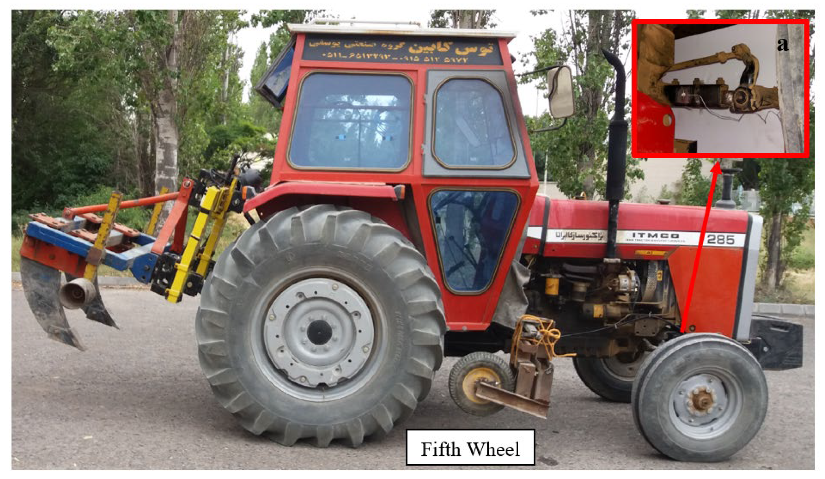
The fuel consumption during the tillage process was measured by two current sensors of OVAL M-III type (LSF 40; Kamiochiai 3-chome Shinjuku-ku, Tokyo; Japan). One of the sensors was employed to measure the input fuel to the injector pump while the second one measured the amount of fuel returning from the fuel cycle to the fuel tank. Both sensors were connected to a temporal fuel consumption display (FM101-50, Tehran, Iran) (Figure 1). This display was connected to the data acquisition system using a cable. The fuel consumption was obtained based on two fuel consumption indices: temporal fuel consumption (TFC) and specific fuel consumption (SFC) using the following equation:
SFC = TFC P db
Pdb: drawbar power (kW)
TFC: Temporal fuel consumption (L/h)
SFC: specific fuel consumption (L/h·KW)
A manual conic penetrometer (CP40II, RIMIK electronic, Rimik, 1079 Ruthven St, Toowoomba, QLD 4350, Australia RIMIK Electronic) was used to measure the cone index. The cone index was calculated based on the force measured to push a cone with a cross-section of 133 mm2 with a tip angle of 30° into the soil. The operator could tune the speed of cone penetration and continuously obtain the cone index in the depth range of 0 to 50 cm. The data acquisition system included a digital programmable data logger (ATRON, AL-8G Tehran, Iran) with 8 channels (Figure 2), and a laptop (Dell Inspiron 1545, Beijing, China) which was located inside the driver chamber. The moisture content of the soil was measured after sampling the soil from different depths using a sensitive electronic balance, followed by their drying at 105 °C for 24 h. Afterward, the soil samples were remeasured, and their moisture content was determined by the following equation:
M c = W W W d W d × 100
where Ww and Wd, respectively, show the wet and dry weight of the soil in grams.
A conventional tillage system comprising a C-shaped two-branch subsoiler (Taka, 220, Arak, Iran) and a 75-horse power FWD tractor (MF-285, Tabriz, Iran) with a tire specification of 18.4/15–30 (ten layers) was used which was equipped with precise measurement tools. Forward speed, temporal fuel consumption, and dynamic load on the front wheels were measured during the tillage process. The specifications of the tractor and subsoiler are shown in Table 1 and Table 2. The precise measurement system was equipped with a fifth wheel velocity measurement sensor, a sensor to measure the dynamic load (strain-gauges on the frontal axis), two fuel sensors, and a data acquisition system (Figure 2 and Figure 3).

2.2. Field Experiments

Field experiments were carried out in the research and education fields of Mohaghegh Ardabili University for two soil types: sandy clay loam and clay. The tests were designed in a factorial manner based on RCBD in triplicates. For each soil texture, various moisture contents (8–17% for dry and 18–40% for moist soils), forward speeds (1.2, 1.6. 1.8, and 2.2 km h−1), working depths (30 and 50 cm), the number of passes (2 and 6), and tire inflation pressure (20 and 25 psi) were considered, and cone index, dynamic load, moisture content, and TFC were measured for each section. The data were then analyzed after being transferred to the computer.

2.3. Neural Network Design

A CNN was used to predict the fuel consumption of the tractor. The results of the current study indicated that the neural network developed based on the Sgdm algorithm outperformed the others; thus, it was selected for modeling. Multi-layer networks have shown promising outcomes in terms of prediction if they have a sufficient number of neurons in their hidden layer. There is no general consensus on the number of the hidden layers and their neuron population. The decision on the number of the neurons in the middle layers is based on trial and error. In this work, the number of hidden layers and their neurons were selected relative to the number of neurons in the middle layers based on comparing the performance of the networks. A linear transfer function was employed due to its better performance. The designed model has eight inputs and one output. Figure 4 shows a schematic of the network architecture. The input and output data were normalized in the range of −1 to 1 to increase the accuracy and speed of the model:
X n = 2 X X min X max X min 1
where Xn and X, respectively, denote the normalized and raw input variables. Xmin and Xmax also show the minimum and maximum input variables, respectively.
The performance of the trained neural network was investigated by comparing the actual outputs with the predicted ones. The choice of the best training method and comparison of the developed networks were based on MSE and R2 values of the linear fitting of the actual and predicted data. The following equations show how the mentioned statistical parameters are determined:
MSE = 1 n i = 1 n Y predicted Y actual 2
  R 2 = i = 1 n Y predicted Y actual 2 i = 1 n Y predicted Y mean 2
where Y actual   and Y predicted   are the actual and predicted values, respectively.

2.4. Data Used in the Designed CNN

The choice of the data for training the network is the most important factor in the design of neural networks. The elements of the input vectors should be selected such that they can describe the conditions governing the system well. As the aim of the ANN in this research was to predict the temporal and specific fuel consumption, the input vectors were selected among the effective parameters. In this study, the input parameters of the ANN include soil moisture content, forward speed of the tractor, cone index of the soil, working depth of the blade, the number of the pass of the tractor wheel, tire inflation pressure, and dynamic load on the front wheels. The data obtained from the field experiments were used. In this study, 70% of the data were employed to train the network while 15% of the data were utilized for validation. The remaining 15% were used for testing.

3. Results and Discussion

As mentioned earlier, a CNN was applied in this research to model the temporal and specific fuel consumption of the tractor wheels. The results indicated that the neural network developed based on the Sgdm algorithm outperformed the others; therefore, it was utilized for modeling the results. MATLAB 2021a was employed to program the designed CNN, while R2 and MSE were considered for evaluation.

3.1. Temporal Fuel Consumption

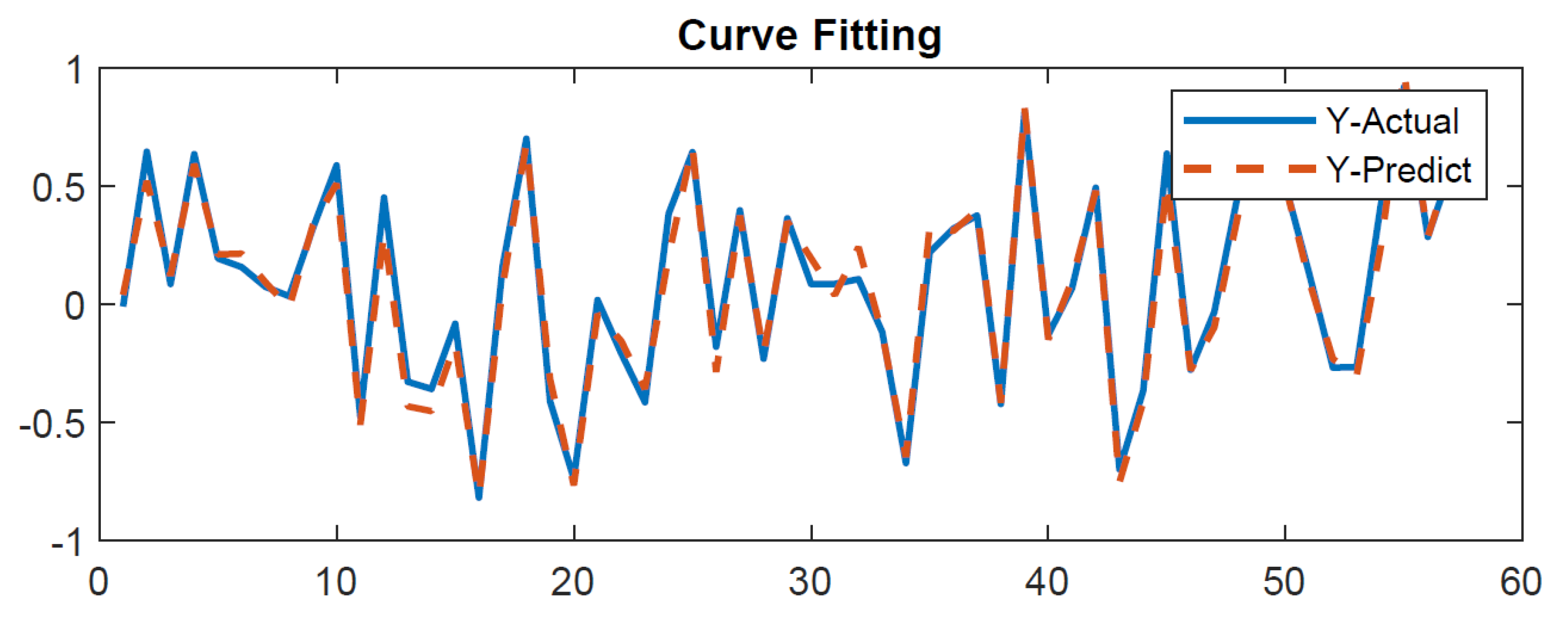
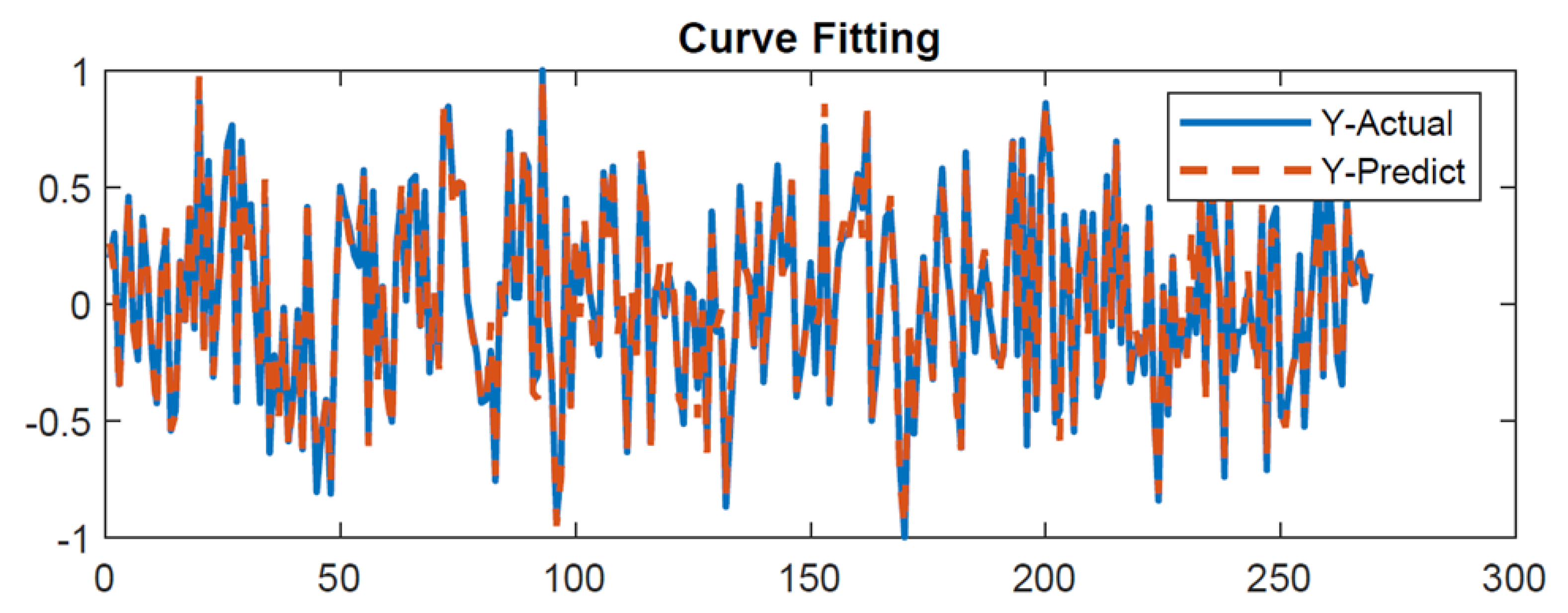
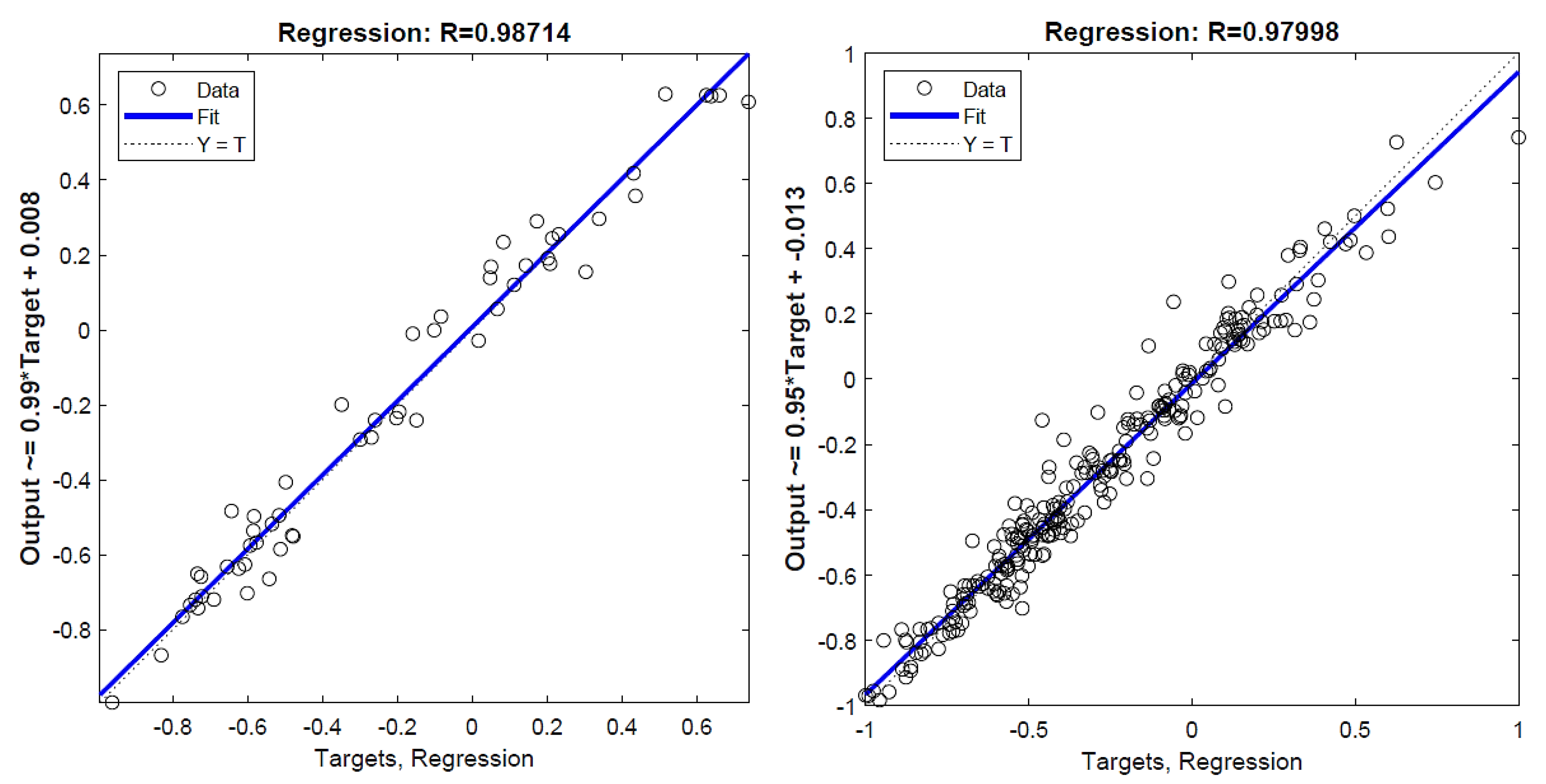
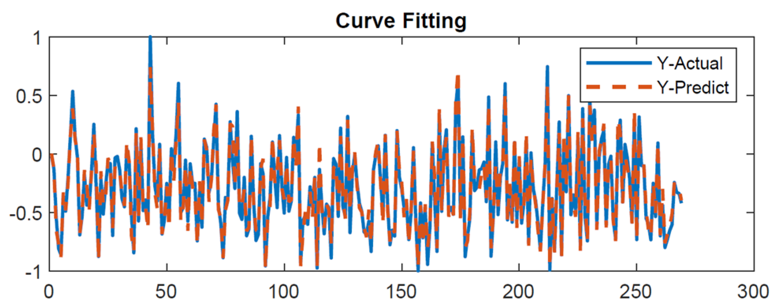
Figure 5 shows the results of the best regression model with an 8-510-510-1 algorithm for prediction of the temporal fuel consumption with R2 of 0.9716 and 0.9729 and MSE of 0. 0047 and 0.0049 for the training and test steps, respectively. The proximity of the real and modeled data confirms the accuracy of the CNN model. Abed Dhahad et al. [4] obtained similar results. They developed an intelligent technique for predicting internal combustion performance, emissions, and combustion characteristics of diesel engines. They used a multi-layer feedforward artificial neural network with particle swarm optimization to model the relationship among engine emissions and operating parameters of direct injection diesel engines. For brake-specific fuel consumption, the highest correlation coefficient was 0.999 and the lowest RMSE was 1.47. In another study, Mustayen et al. [5] developed a single-zone thermodynamic model to predict the engine performances such as brake power (BP), torque, brake thermal efficiency (BTE), brake-specific fuel consumption (BSFC), and ignition delay (ID) times for diesel and jojoba biodiesel. The performance simulation results agreed with experimental data for all tested fuels at 1200 to 2400 rpm speed and 25, 50, 75, and 100% loading operation. The minimum error (3.7%) was observed for BP for D100 at 2000 rpm and 100% load, and the maximum error (19.2%) was found for JB10 at 1200 rpm and 25% loading operation. The results of the research showed that the BSFC increased with increasing speed due to increased friction power and more fuel consumption. BSFC then decreases with increasing load because of higher combustion efficiency and more BP produced at higher load operation. In addition, jojoba–diesel blends show a higher BSFC than diesel fuel due to their high density and lower calorific value. Almaliki et al. [7] reported similar results in prediction of the temporal fuel consumption of a Massey Fergusson 285 tractor equipped with a moldboard plow using an ANN. The 6-7-1 architecture with the Levenberg–Marquart training algorithm showed the best performance in prediction of the temporal fuel consumption with R2 = 0.969 and MSE = 0.1342. Fathollahzedeh et al. [19] examined the temporal fuel consumption of a John Deere tractor (3140) equipped with a moldboard plow in various work depths. They reported a linear relationship between the fuel consumption and working depth with R2 = 0.987. In another study by Moitzi et al. [20], the effects of the depth, slippage, engine speed, and forward speed were evaluated on the fuel consumption of a four-wheel tractor equipped with several agricultural tools (reversible moldboard plow, short disc harrow, universal-cultivator, subsoiler). The highest R2 values (0.999) were for the short disc harrow and reversible moldboard plow for depth-fuel consumption rate (Lh−1). The difference between the results of this research with other studies can be assigned to the high number of input parameters and hence the complexity of the CNN. This study indicated that all the input parameters of the CNN can affect the temporal fuel consumption. Figure 6 and Figure 7 compare the experimental and modeled values of temporal fuel consumption for the test and training stages, respectively. These diagrams confirm the consistency between the real and CNN-modeled values during the experiments in the test stage.

3.2. Specific Fuel Consumption

Figure 8 depicts the best regression model for training and testing specific fuel consumption. As can be seen, the data are scattered around a line with high approximation. The proximity of the real and modeled data confirms the accuracy of the CNN. The best structure of a CNN with architecture of 8-100-95-1 led to R2 values of 0.9603 and 0.9737 and MSE of 0.0055 and 0.0054 for the training and test steps, respectively. These results are similar to the reports by Almaliki et al. [7] who predicted the SFC of a Massey Ferguson 285 tractor equipped with a moldboard plow using an ANN. The best structure was obtained with the architecture of 6-10-1 with the Levenberg–Marquart training algorithm with the R2 value of 0.935 and MSE of 0.0127. Küçüksarıyıldız et al. [21] predicted the specific fuel consumption of a 60 hp front-wheel drive tractor using an artificial neural network. The independent parameters included the dynamic load on the axle (1796, 2076, 2276, and 2476 daN), tire inflation pressure (80, 120, and 160 KPa), and traction force (500, 1000, 1500, and 2000 daN). For a constant dynamic load level and constant tire inflation pressure, they obtained a relationship between specific fuel consumption and traction force as a second-order curve (with R2 = 0.97). Regarding the large number of input parameters in this research, the obtained results are rational and reasonable compared to the results of others. The results also reflect that all input parameters affect the fuel consumption. Figure 9 and Figure 10 show the curve fitting for the target values against the output values of the CNN for the specific fuel consumption for the test and training data, respectively. They demonstrate the consistency between the actual and the modeled values during the number of experiments in the test phase by the convolutional neural network.

4. Conclusions

The current research shows the prediction of temporal fuel consumption and specific fuel consumption of a tractor by a convolutional neural network. MSE and R2 statistical criteria were used to assess the performance of the model. The results of this research showed the better performance of the neural network developed based on the Sgdm; therefore, this algorithm was used for modeling. The best performance for temporal fuel consumption was obtained with the 8-510-510-1 architecture with R2 of 0.9729 and MSE of 0.0049. Furthermore, for the specific fuel consumption, 8-100-95-1 architecture showed the best performance with R2 of 0.9737 and MSE of 0.0054. The difference between the results of this research and other studies can be attributed to the large number of input parameters and the complexity of the convolutional neural network. Table 3 shows the sensitivity analysis of the input parameters and its effects on the output parameters. Moreover, the results proved that all network input parameters affect the instant fuel consumption and specific fuel consumption. The results also indicated that convolutional neural networks can learn the relationship between the input and output variables of tractor fuel consumption well. Regarding the complexity between the variables and the absence of a specific relationship between the parameters, this network with its large number of hidden layers and neurons can be used for prediction and modeling. As these networks are generally used for image classification, they can be used for modeling and predicting features by removing the convolution layers and the dimension reduction layers. So far, no research has used this method to predict fuel consumption. The high prediction accuracy and low error in this research compared to previous studies indicate the superiority of this method in order to predict fuel consumption. It was also observed from the results that the input parameters, which include soil and operational parameters, are all effective on fuel consumption. Proper management of some parameters, such as plowing depth, tire inflation pressure, and forward speed, can help to optimize fuel consumption.
It is expected that future research, at the same time as predicting the amount of tractor fuel consumption in different load conditions, will also deal with the amount of pollution and suspended particles.

Author Contributions

Conceptualization, H.J., Y.A.-G., V.R.-S. and A.M.; methodology, H.J., Y.A.-G., V.R.-S. and A.M.; software, H.J. and Y.A.-G.; validation, H.J., Y.A.-G., V.R.-S., A.M. and J.L.H.-H.; formal analysis, H.J., Y.A.-G., V.R.-S. and A.M.; investigation, H.J., Y.A.-G., V.R.-S., A.M., J.L.H.-H., M.H.-H. and J.A.M.-V.; resources, H.J., Y.A.-G., V.R.-S., A.M., J.L.H.-H., M.H.-H. and J.A.M.-V.; data curation, H.J. and Y.A.-G.; writing—original draft preparation, H.J., Y.A.-G., V.R.-S. and A.M.; writing—review and editing, J.L.H.-H., M.H.-H. and J.A.M.-V.; visualization, H.J., Y.A.-G., V.R.-S. and A.M.; supervision, Y.A.-G.; project administration, Y.A.-G.; funding acquisition, Y.A.-G., J.A.M.-V., J.L.H.-H. and M.H.-H. All authors have read and agreed to the published version of the manuscript.

Funding

This research was funded by University of Mohaghegh Ardabili under project number of 51-11031/1399-05-07.

Institutional Review Board Statement

Not applicable.

Informed Consent Statement

Not applicable.

Data Availability Statement

The data presented in this study are available on request from the corresponding author.

Conflicts of Interest

The authors declare no conflict of interest.

References

  1. Šmerda, T.; Čupera, J. Tire inflation and its influence on drawbar characteristics and performance–Energetic indicators of a tractor set. J. Terramech. 2010, 47, 395–400. [Google Scholar] [CrossRef]
  2. Elwaleed, A.K.; Yahya, A.; Zohadie, M.; Ahmad, D.; Kheiralla, A.F. Net traction ratio prediction for high-lug agricultural tyre. J. Terramech. 2006, 43, 119–139. [Google Scholar] [CrossRef]
  3. Çarman, K.; Taner, A. Prediction of tire tractive performance by using artificial neural networks. Math. Comput. Appl. 2012, 17, 182–192. [Google Scholar] [CrossRef]
  4. Abed Dhadah, H.; Ahmed Mudheher, H.; Miqdam Tariq, C.; Hussein, A.K. Prognostic of diesel engine emissions and performance based on an intelligent technique for nanoparticle additives. Energy 2022, 238, 121855. [Google Scholar] [CrossRef]
  5. Mustayen, A.G.M.B.; Rasul, M.G.; Wang, X.; Bhuiya, M.M.K.; Negnevitsky, M.; Hamilton, J. Theoretical and Experimental Analysis of Engine Performance and Emissions Fuelled with Jojoba Biodiesel. Energies 2022, 15, 6282. [Google Scholar] [CrossRef]
  6. Rahimi-Ajdadi, F.; Abbaspour-Gilandeh, Y. Artificial neural network and stepwise multiple range regression methods for prediction of tractor fuel consumption. Measurement 2011, 44, 2104–2111. [Google Scholar] [CrossRef]
  7. Almaliki, S.; Alimardani, R.; Omid, M. Artificial neural network based modeling of tractor performance at different field conditions. Agric. Eng. Int. CIGR J. 2016, 18, 262–274. [Google Scholar]
  8. Igoni, A.H.; Ekemube, R.A.; Nkakini, S.O. Predicting tractor fuel consumption during ridging on a sandy loam soil in a humid tropical climate. J. Eng. Technol. Res. 2019, 11, 29–40. [Google Scholar] [CrossRef]
  9. Siddique, M.A.A.; Baek, S.-M.; Baek, S.-Y.; Kim, W.-S.; Kim, Y.-S.; Kim, Y.-J.; Lee, D.-H.; Lee, K.-H.; Hwang, J.-Y. Simulation of Fuel Consumption Based on Engine Load Level of a 95 kW Partial Power-Shift Transmission Tractor. Agriculture 2021, 11, 276. [Google Scholar] [CrossRef]
  10. Kolator, B.A. Modeling of Tractor Fuel Consumption. Energies 2021, 14, 2300. [Google Scholar] [CrossRef]
  11. LeCun, Y.; Bengio, Y.; Hinton, G. Deep learning. Nature 2015, 521, 436–444. [Google Scholar] [CrossRef]
  12. Zhang, Z.; Cui, P.; Zhu, W. Deep learning on graphs: A survey. IEEE Trans. Knowl. Data Eng. 2020, 34, 249–270. [Google Scholar] [CrossRef]
  13. Yao, G.; Lei, T.; Zhong, J. A review of convolutional-neural-network-based action recognition. Pattern Recognit. Lett. 2019, 118, 14–22. [Google Scholar] [CrossRef]
  14. Dhillon, A.; Verma, G.K. Convolutional neural network: A review of models, methodologies and applications to object detection. Prog. Artif. Intell. 2020, 9, 85–112. [Google Scholar] [CrossRef]
  15. Chen, Y.; Wei, Y.; Wang, Q.; Chen, F.; Lu, C.; Lei, S. Mapping post-earthquake landslide susceptibility: A U-Net like approach. Remote Sens. 2020, 12, 2767. [Google Scholar] [CrossRef]
  16. Wang, N.; Chen, F.; Yu, B.; Qin, Y. Segmentation of large-scale remotely sensed images on a Spark platform: A strategy for handling massive image tiles with the MapReduce model. ISPRS J. Photogramm. Remote Sens. 2020, 162, 137–147. [Google Scholar] [CrossRef]
  17. Tsakiridis, N.L.; Keramaris, K.D.; Theocharis, J.B.; Zalidis, G.C. Simultaneous prediction of soil properties from VNIR-SWIR spectra using a localized multi-channel 1-D convolutional neural network. Geoderma 2020, 367, 114208. [Google Scholar] [CrossRef]
  18. Zhang, X.; Lin, T.; Xu, J.; Luo, X.; Ying, Y. Deep Spectra: An end-to-end deep learning approach for quantitative spectral analysis. Anal. Chim. Acta 2019, 1058, 48–57. [Google Scholar] [CrossRef]
  19. Fathollahzadeh, H.; Mobli, H.; Rajabipour, A.; Minaee, S.; Jafari, A.; Tabatabaie, S.M.H. Average and instantaneous fuel consumption of Iranian conventional tractor with mouldboard plow in tillage. ARPN J. Eng. Appl. Sci. 2010, 5, 30–35. [Google Scholar]
  20. Moitzi, G.; Wagentristl, K.; Refenner, K.; Weingartmann, H.; Piringer, G.; Boxberger, J.; Gronauer, A. Effects of working depth and wheel slip on fuel consumption of selected tillage implements. Agric. Eng. Int. CIGR J. 2014, 16, 182–190. [Google Scholar]
  21. Küçüksarıyıldız, H.; Çarman, K.; Sabancı, K. Prediction of Specific Fuel Consumption of 60 HP 2WD Tractor Using Artificial Neural Networks. Int. J. Automot. Sci. Technol. 2021, 5, 436–444. [Google Scholar] [CrossRef]
Figure 1. (a) The tractor equipped with a precise measurement system; (b,c) fuel sensors used in this research.
Resources 12 00046 g001
Figure 2. The data acquisition system and fuel consumption display system inside the driver cabin.
Resources 12 00046 g002
Figure 3. Tractor equipped with the precise measurement system and (a) strain-gauges installed on the frontal excel of the tractor.
Resources 12 00046 g003
Figure 4. A schematic representation of the applied CNN.
Resources 12 00046 g004
Figure 5. Regression of the best CNN for temporal fuel consumption in the training (right) and test (left) steps.
Resources 12 00046 g005
Figure 6. Comparison between the actual and predicted temporal fuel consumption vs. the number of experiments in the test step.
Resources 12 00046 g006
Figure 7. A comparison between the actual and predicted temporal fuel consumption vs. the number of experiments in the training stage.
Resources 12 00046 g007
Figure 8. Regression of the best CNN for prediction of SFC in the training (right) and test (left) phases.
Resources 12 00046 g008
Figure 9. A comparison of the actual and CNN-predicted SFC vs. the number of experiments in the test phase.
Resources 12 00046 g009
Figure 10. A comparison between the real and predicted SFC vs. the number of experiments in the training phase.
Resources 12 00046 g010
Table 1. Specifications of Massey Ferguson tractor (MF285).
ItemParameters
ManufacturerMotor manufacturer’s company
TypeDiesel with direct injection
Number of cylinders4
Compression ratio16:1
Firing order11-3-4-2
Maximum power at 2000 rpm75 hp
Maximum torque at 1300 rpm278 N·m
Type of injector pumpRotary
Fuel tank capacity90 L
TransmissionGears
Lifting capacity2227 kg
Type of steering systemMechanical-hydraulic
Type of cooling systemLiquid-cooled
Type of injector pumpRotary
Distance to the ground380 mm
Front tire size12.4–24 inch
Rear tire size18.4/15–30 inch
Disc weights on the rear wheel180 kg
Bag weights in front of the tractor192 kg
Front weight1350 kg
Rear weight1820 kg
Total weight3170 kg
Table 2. Specifications of subsoiler.
ModelTaka 220
Working width1.3 m
Maximum working depth50 cm
Power required75 hp
Number of branches2
Branch spacing35–65 cm
The weight of the device300 kg
The length of the device90 cm
Device height120 cm
The width of the device during transportation120 cm
Table 3. Sensitivity analysis of parameters affecting fuel consumption.
Input ParametersValueTFC
(L·h−1)
SFC
(L·kw−1·h−1)
Soil MoistureDry17.62.21
Wet19.472.24
Soil Texturesandy clay loam17.22.14
clay19.872.19
Working Depth30 cm17.012.02
50 cm20.052.28
Forward Speed1.2 km h−115.582.74
1.6 km h−116.91.73
1.8 km h−1202.47
2.2 km h−121.61.73
Number of Passes219.482.32
617.62.01
Inflation Pressure25 psi16.791.99
20 psi20.282.34
Cone Index2.377 MPa16.111.98
1.776 MPa17.912.1
2.822 MPa19.522.23
2.039 MPa21.012.35
Dynamic Load5817.31 N18.042.19
6380.31 N20.912.44
6254.46 N15.391.89
6728.93 N19.172.14
Disclaimer/Publisher’s Note: The statements, opinions and data contained in all publications are solely those of the individual author(s) and contributor(s) and not of MDPI and/or the editor(s). MDPI and/or the editor(s) disclaim responsibility for any injury to people or property resulting from any ideas, methods, instructions or products referred to in the content.