Article

Multivariate Analysis of Geological Data for Regional Studies of Geodiversity

1
Norwegian Institute for Nature Research, NO-0855 Oslo, Norway
2
Geological Survey of Norway, NO-7491 Trondheim, Norway
3
Geological Survey of Sweden, SE-75128 Uppsala, Sweden
*
Author to whom correspondence should be addressed.
Resources 2022, 11(6), 51; https://doi.org/10.3390/resources11060051
Submission received: 12 April 2022 / Revised: 10 May 2022 / Accepted: 18 May 2022 / Published: 24 May 2022
(This article belongs to the Special Issue Geodiversity Assessment: What, Why and How?)

Abstract

:
In Norway, a landscape map exists which gives the opportunity to collect data in landscape units for further analysis. This study covers parts of Norway and Sweden, so the landscape map was extended into Sweden to form a unified landscape structure. A collection of geological and terrain data within landscape units can serve as a tool to describe the geodiversity profile of the units, study their geographical distribution and analyse similarities and dissimilarities between them. We collected geological and terrain data for an area covering large parts of southern Norway and Sweden. The data were collected as attributes in landscape polygons. The data were then analysed using multivariate techniques (Principle component analyses) where the first four axes of variation were definable. The first axis is a terrain axis, the second a bedrock unit axis, the third a bedrock diversity axis and the fourth a soil/sediment axis. In total, the four gradients answer for 54.9% of the total variation in the material. Links are found between the terrain data and geological units, but these links are relatively weak. The four gradients represent a step-less model of the geodiversity profile of the landscape areas but are dependent on the quality and scale of the input data. Norwegian and Swedish data had to be harmonised in order to be analysed together; however, because of this they ended up having a coarser resolution than desired, both spatially and scientifically. The stepless model was clustered to form 16 geodiversity profile groups for easy comparison and regional overview. The procedure can serve as a baseline for more detailed and field-based studies of geodiversity profiles, and give the opportunity to make analytical maps through simple overlay techniques and to compare areas with each other with respect to their geodiversity profile. This can be carried out both alone and in a wider landscape setting.

1. Introduction

The diversity of nature consists of two major elements, biodiversity and geodiversity. Biodiversity has existed as a term both scientifically and politically for a long time. Geodiversity is a somewhat newer term that has established itself on par with biodiversity. It is, however, far from as established within the broad scientific or political nomenclature. Perhaps the most common and simplest definition of geodiversity is given by [1]: “the natural range (diversity) of geological (rocks, minerals, fossils), geomorphological (landforms, topography, physical processes), soil and hydrological features. It includes their assemblages, structures, systems and contributions to landscapes.” This is a modification of a definition used in Australia [2] and is very similar to the definition used previously in the Nordic countries [3]. Several other definitions have emerged, mostly related to the degree of scientific specifications.
Diversity in this respect has been considered as a useful term, but it is constantly under debate. One major reason for this dispute is intrinsic to the term; it expresses a vast variation in elements, scales and conditions [4]. Thus, a multitude of perspectives exist and several papers concerning diversity have a focus on parts of the total diversity or on limited areas [5,6,7]. Examples from biodiversity may be species diversity or the diversity of vascular plants, and for geodiversity this includes landform diversity and bedrock diversity.
As has been the case with biodiversity [8,9], different indices expressing key characteristics of geodiversity have been developed [10,11,12,13]. They are typically used as an element in assessing or describing key aspects of a defined area, and to facilitate comparison between areas [7]. A key issue and an obstacle in using such indices over larger areas is the strong intrinsic scale dependence of these attributes and the challenge in the availability of relevant data over large areas.
This paper aims to explore the possibility to develop a GIS-based representation of key geodiversity elements on a regional scale that will provide a foundation for comparison between areas and serve as a basis for more detailed studies in the distribution of geodiversity attributes. Our approach is based on improved data availability and digital mapping methods. This study does not present a new or revised geodiversity index, but rather a method of analysing available data as a platform for further assessment. The study is based on existing data from geodatabases containing bedrock and soil information (Quaternary geological maps) and terrain data derived from elevation databases. These sources of information are steadily developing in quality and content. The aim of the paper is to extend the datasets of previous studies by collecting more and better data, and to analyse these in a landscape setting. In this way we hope to strengthen the understanding of the relevance of these datasets for geodiversity analysis, as well as create opportunities for new analysis whenever datasets are improved or new data become available.

2. Material and Methods

2.1. Study Area

The study area is an approximately 120,000 km2-large cross-border region between Norway and Sweden and covers large parts of the southern Scandinavian peninsula (Figure 1). The area crosses a zone of rocks representing the Sweconorwegian, Swecokarelian and the Caledonian orogeny [14]. This represents a gradient of the Tertiary uplift history in Scandinavia from maximum uplift to the west to minimum uplift in the east and has a central position in the last Weichselian glaciation [15,16]. Excluding the outer coastal areas on both sides, it represents a profile through the southern Scandinavian inland. In the northwest, the terrain rises to above 2000 m.a.s.l., and in the east/southeast large areas are dominated by low-lying terrain with typical altitudes below 200–400 m.a.s.l.

2.2. Geology

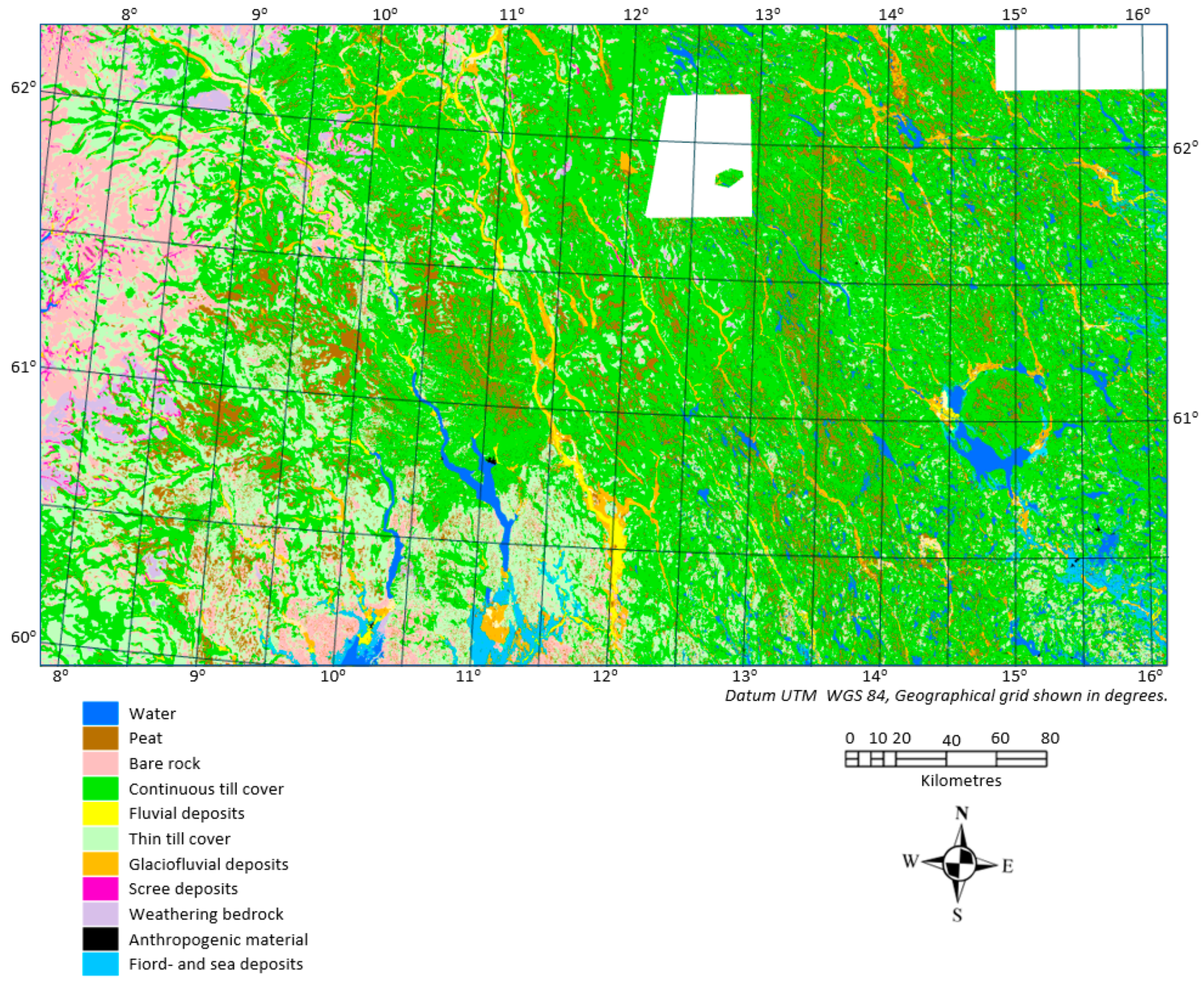
The main rock types found in the study area are granite/granitic gneisses and sandstones with different degrees of consolidation [15,17]. In addition, the bedrock in the area consists of acidic and basic intrusive rocks, basic metamorphosed rocks, mica-rich sedimentary and metamorphic rocks and various volcanic rocks (Figure 1). The area also includes an eroded large meteorite impact structure. Till cover dominates in large parts of the area with peat, glacifluvial and fluvial sediments adding to soil diversity (Figure 2). In high areas in the west bare rock can dominate, and in the east and west marine sediments are important.
During the deglaciation following the last glacial maximum, the main ice divide in South Scandinavia was situated south of the main water divide. This led to the formation of large ice-dammed lakes and subsequently lake deposits in the study area. When these lakes drained, extensive meltwater erosional landforms were formed. This is visible today as a multitude of glaciolacustrine sediments and glaciofluvial landforms such as deltas, eskers, drainage channels, etc. [16,18]. There are differences in the quality of mapping as well as the interpretation of detailed geological features on each side of the national border. Thus, to develop harmonised, trans-national data sets, we need to simplify and utilise regional data as the lowest common denominator rather than data of the highest quality in either country. This may lead to data loss for detailed structures and features.

2.3. Landscape Types and Landscape Areas

As a part of a large initiative for a new nature description system in Norway [19], a new landscape classification system was developed. At the same time, a new GIS-based landscape map covering all of Norway was constructed [20]. The landscape classification system is based on an extensive numerical analysis of many variables, including most of what is available of data covering all areas of Norway, spanning from terrain through geology, soil, vegetation and human landcover [21]. The landscapes are divided into three groups: marine landscapes, coastal landscapes, and inland landscapes. Nine major landscape types have been established, three for each of the main groups, plains, valleys, and hill/mountain landscapes (for definitions see the above references). The major landscape types are divided into minor types according to landscape gradients identified through multivariate analysis. These gradients are uniquely defined for each major landscape type and consist of attributes representing aspects of geodiversity, biodiversity and human land use. The minor types are defined as collections of the smallest units in the landscape map, called landscape areas, which have the same characteristics according to the relevant landscape gradients. It is these landscape areas that are used as the basic data-collection polygons in this study. This leads to maps divided into polygons covering the whole area of investigation. The landscape areas are spatially defined through a simple GIS hydrological basin model [22] applied within each landscape major type using an elevation model. For the hill and mountain landscape, the method has been used on an inverted basin model. The procedure is described in detail in reference [21].
The landscape area map that was used as a base information layer in this study contains data that represent their physical properties. This includes major geomorphic attributes such relief, valley form, the presence of bogs and lakes and their major classification in fjord, inland plains, valley, and hill and mountain landscapes [20]. This represents important geodiversity characteristics of the land and in our setting served as the backbone of our analysis.
LiDAR terrain data were not available when the landscape type map was created, so an interpolated DEM with a resolution of 100 m based on 20 m contour intervals was used. Geological data and soil data were available at a scale of 1: 250,000, but in the multivariate analysis no landscape gradients containing these data were then identified [20]. We have now collected supplementary geological and terrain data as additional attributes in the same landscape area polygons. With simple GIS overlay techniques, the range of geological information that can be used as landscape attributes can be extended as much as we want or have available data for. It is, however, difficult to manually assess the relevance of each attribute, especially when we want to compare different areas with others.
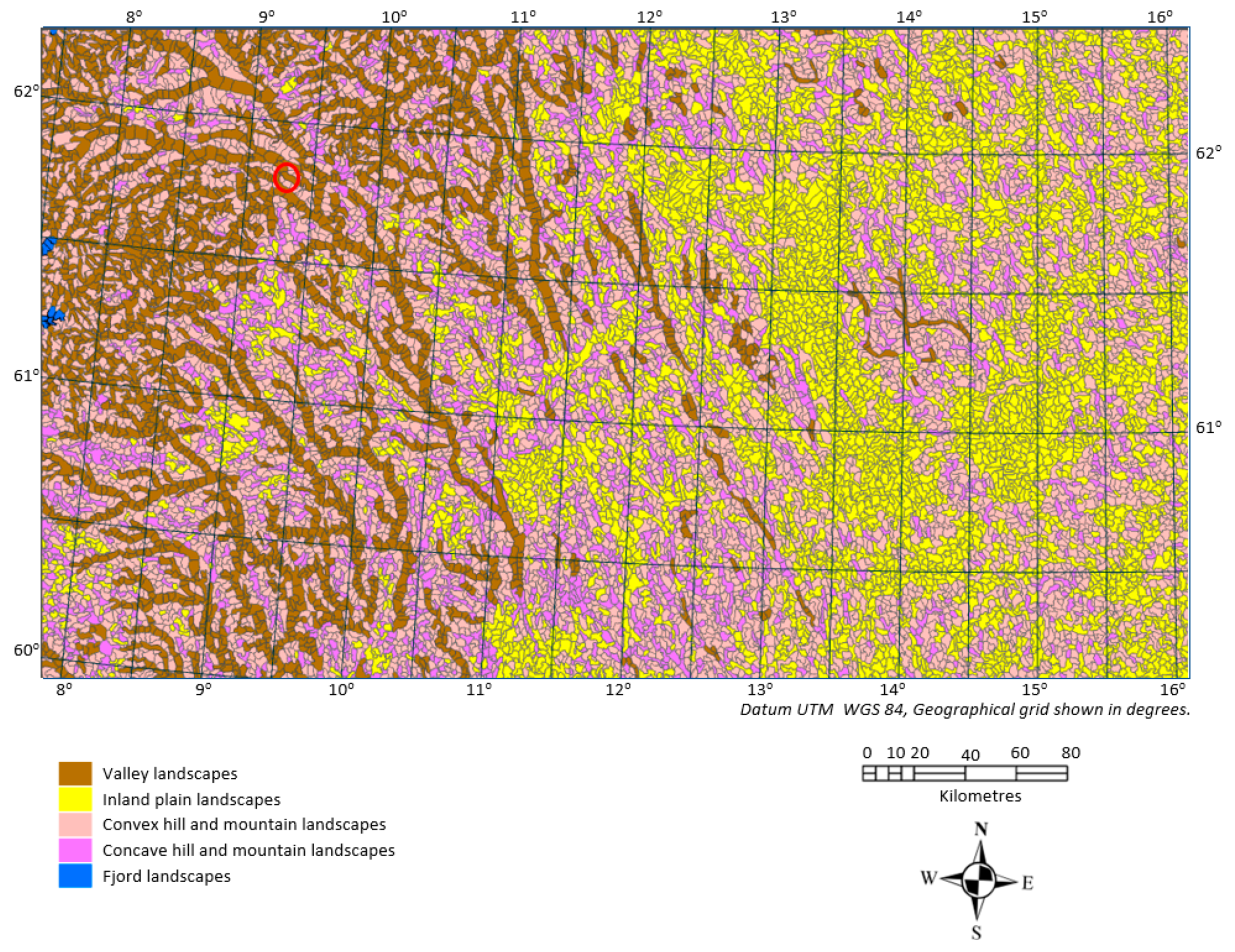
The landscape area map exists only for Norway, so to perform the analysis for all of the study area, the same algorithms were used for the Swedish territory and the two parts were then merged into one map (Figure 3). The polygons on each side of the border show a good match, which indicates that the algorithms used are robust and the method reproducible. This map has 14,474 polygons with a median size of 7.5 km2. The largest polygon is nearly 60 km2 in size and there exist 143 polygons smaller than 1 km2. All of these <1 km2 polygons are edge polygons resulting from the cutting of a larger polygon by the border of the investigation area.
For the analysis we used terrain data from three resolutions of elevation models (100 m, 10 m and 2 m). The 2 m resolution was the finest resolution available for the two countries involved and is based on LiDAR measurements. LiDAR data are not available in some of the Norwegian high mountains resulting in data deficiency for the variables based on this data set. The same applies for soil data in a couple of areas in Sweden.

2.4. Terrain Ruggedness

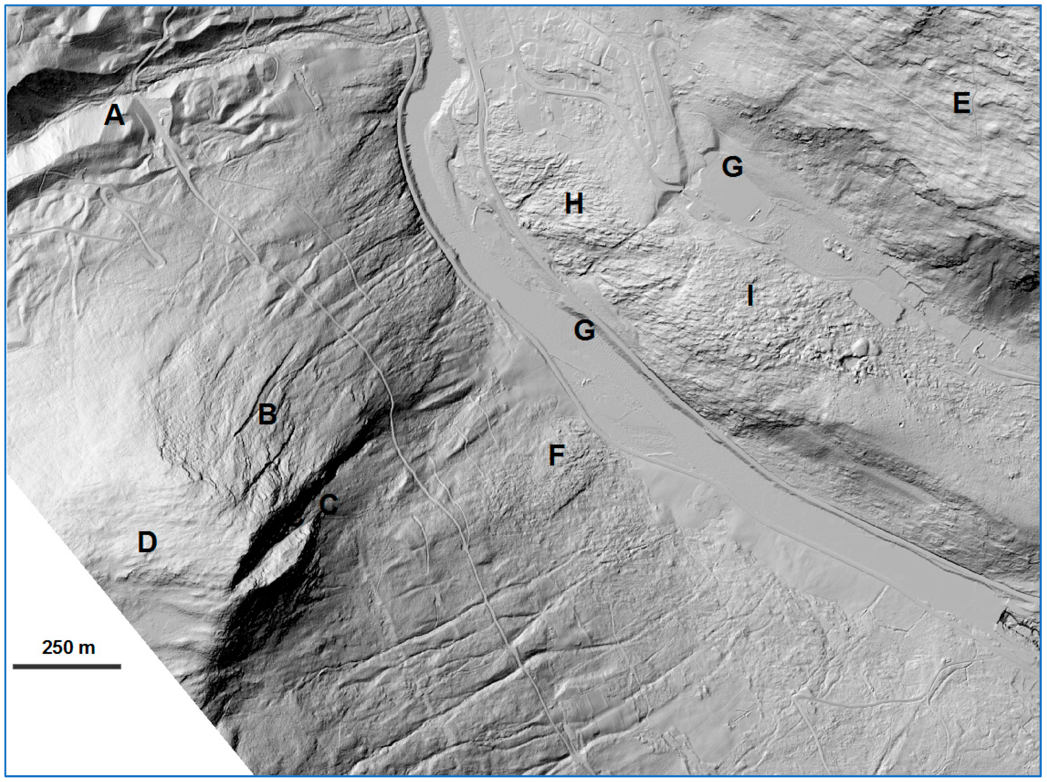
To understand the possibilities for the use of detailed terrain data, we performed a test in a small area in Norway (Figure 3). Terrain ruggedness is an important attribute for landscape characteristics and is closely linked to bedrock structure and landforms, and is therefore of great interest in a geodiversity analysis. The possibility for the detailed representation of terrain ruggedness increases as LiDAR data gradually become more available. There are many indices that measure terrain ruggedness. They are generally very scale-sensitive and it is not very clear what sort of indices represent the best measures in different scales. The aim of this test was to select some indices that capture terrain structure in a very detailed scale. The test area has a terrain diversity that makes it possible within a small area to see how different indices perform.
The test was performed by manual assessment, not statistical analysis, based on an interpretation of terrain structures and ruggedness visualised in a hillshade map from an elevation model with resolution 1 m (Figure 4). The indices used were planform curvature (the mean value of the absolute value of planform curvature, i.e., the horizontal variation of the terrain), aspect diversity (the number of classes of aspect categories (10-degree segments) present, i.e., directional variation), Rough (also called TRI, which measures the elevation difference between a cell in a raster and its neighbouring cells) [23] and VRM, which measures ruggedness including both the vertical and horizontal component of terrain variation [24] (Table 1). All indices were calculated in a circle with a 5-pixels radius. Aspect diversity and VRM seem to be the two best performing indices in capturing small-to-medium-scale ruggedness. Aspect diversity is, however, so sensitive to small changes in terrain that a series of thresholds have to be introduced. We therefore used VRM as the preferred index to capture fine-scale terrain variation. In the final analysis this was supplemented with several other indices and measurements that are commonly used in more coarser scales and that reflect different aspects of terrain variation. The total number of variables used is shown in Table 2.

2.5. Data Preparation for Multivariate Analysis

The data extracted from the landscape area polygons (Figure 3) were all normalised and standardised before being treated with multivariate methods. Altogether 44 variables were sampled and extracted from the GIS using zonal statistics in ArcGIS Pro (Table 2). All variables were then transformed to zero-skewness and kurtosis standardised by division with their expected standard deviations, (6/n)0.5 [27]. Acceptable homogeneity of variances (homoscedasticity) is achieved by transforming all variables to zero skewness.
Three transformation formulae according to [28] were used:
ykj′ = eckxkj
ykj′ = ln(ck + xkj)
ykj′ = ln(ck + ln(ck + xkj))
where xkj is the original value of variable k in plot j and ck is a variable-specific parameter that gives the transformed variable Y′ = {ykj′} zero skewness. The first Equation (1) was applied to left-skewed variables (standardised skewness < 0), the next Equation (2) to right-skewed variables. The last Equation (3) was applied to right-skewed variables for which no ck could be found by the middle equation, which resulted in standardised skewness = 0. After transformation, all variables Y′ were ranged to obtain new variables Y = {ykj} on a 0–1 scale:
ykj = (ykj′ − min(ykj′))/(max(ykj) − min(ykj))

2.6. Principle Component Analyses (PCA) Ordination and Multivariate Clustering

The standardised and normalised matrix was subjected to PCA ordination [29]. PCA was chosen as the ordination method as we assume linear relationships between all the variables included in the analyses. PCA was run on a correlation matrix: a matrix of centred, standardised, and transformed variables. Correlation biplot scaling of PCA axes was used to optimise the fit of angles between variable vectors to intervariable correlations. PCA ordination can be performed by using the vegan package [30] in R software (see Appendix A for code).
We used the spatial statistic tool ‘multivariate clustering’ in ArcGIS Pro to visualise and analyse the principal components (PCs) together. Multivariate clustering finds natural clusters of features based solely on feature attribute values, which here are the values of the principal components.

3. Results

3.1. Ordination Results

The PCA yielded four unconstrained axes which explained 54.9% of the total variation in the material. The cumulative explained variation was 28.71, 41.58, 48.83 and 54.87 for the four axes.
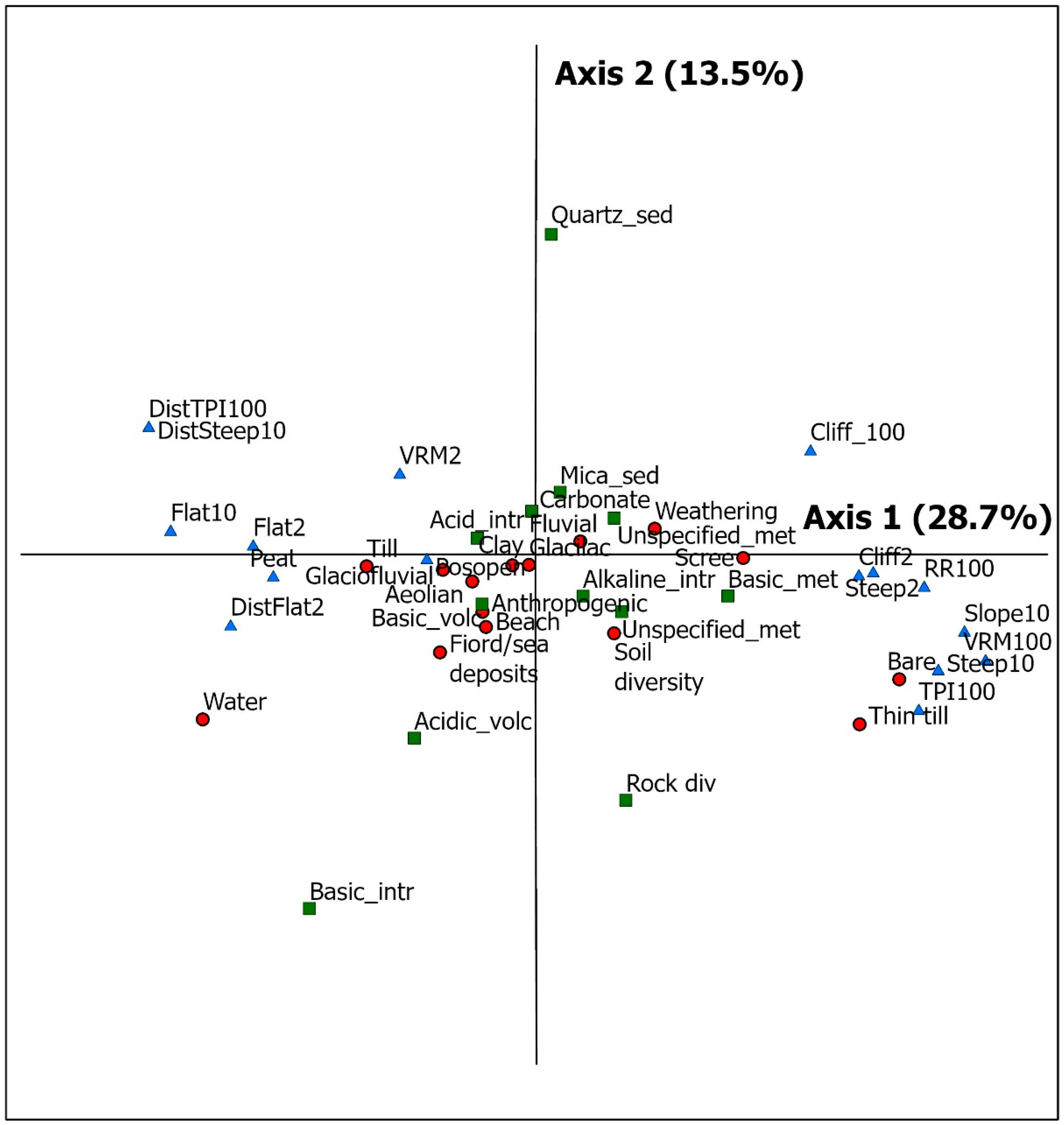
The first axis (Figure 5) sorts out variables along a gradient reflecting the topography within the area, going from lands dominated by steep terrain and high ruggedness having high values, to variables associated with smooth landscapes showing low values along axis 1. Terrain variables on different scales span out the axis systematically without regard to scale/resolution. Landscape elements such as lakes, and geological features such as peatland, glaciofluvial sediments, and thick till cover, have low values and can be associated with flat terrain. Scree, weathering material, bare rock and thin till cover can, on the other hand, be associated with steep terrain, together with basic and ultrabasic rock types such as amphibole.
The second axis spans a gradient heavily influenced by geology. For high values we find quartz- and feldspar-rich sedimentary rock such as sandstones with limestone, shales, and weathering material pulling weakly in the same direction, and ultrabasic, basic and intermediate intrusive rocks such as gabbro, acidic volcanic rock such as granite/granitic gneisses with migmatite, thin till cover and bedrock diversity pulling in the other direction. Topographical variables such as distance to TPI values larger than 15 m at 100 m resolution and distance to steep terrain at 10 m resolution contribute in the direction of quartz-feldspar-rich sedimentary rock. TPI measured in 100 m DEM and steep terrain (10 m) together with thin till and rock diversity contribute in the direction of ultrabasic, basic and intermediate intrusive rocks.
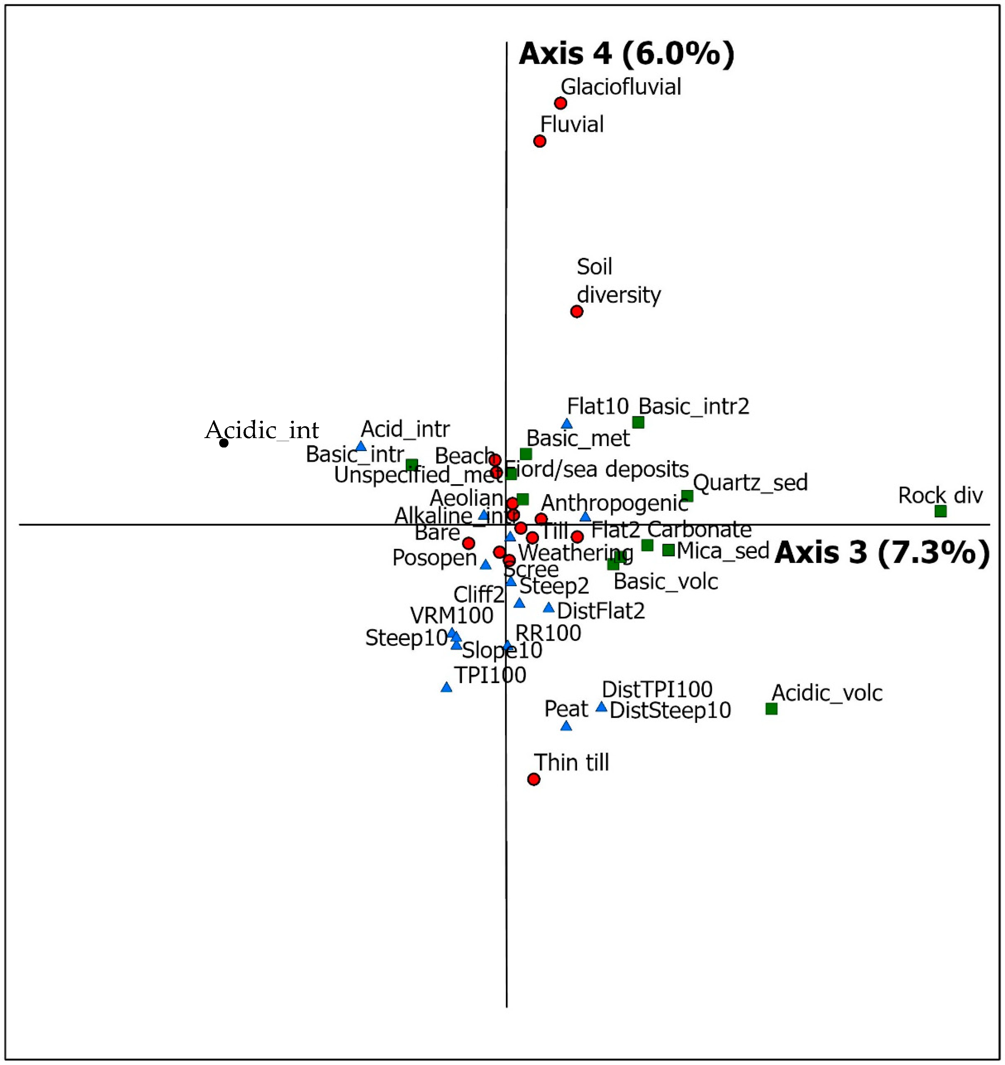
The third axis is heavily influenced by rock type diversity (Figure 6) with ultrabasic, basic and intermediate intrusive rocks on the opposite ends of the axis. Additionally, acidic volcanic rocks have high values along this axis. None of the terrain variables have particularly high positive or negative values along the third axis.
The last gradient sums up a residual (6% explanation rate) and spans a soil gradient with river sediments, glacifluvial sediments and soil diversity with high values and thin till cover and peat, together with distance to steep terrain at 10 m resolution with low values.
It is worth noting that the analysis yields four distinct axes, but that the link between the three geological axes and the topography seems to be rather weak.

3.2. Multivariate Visualisation of the Results

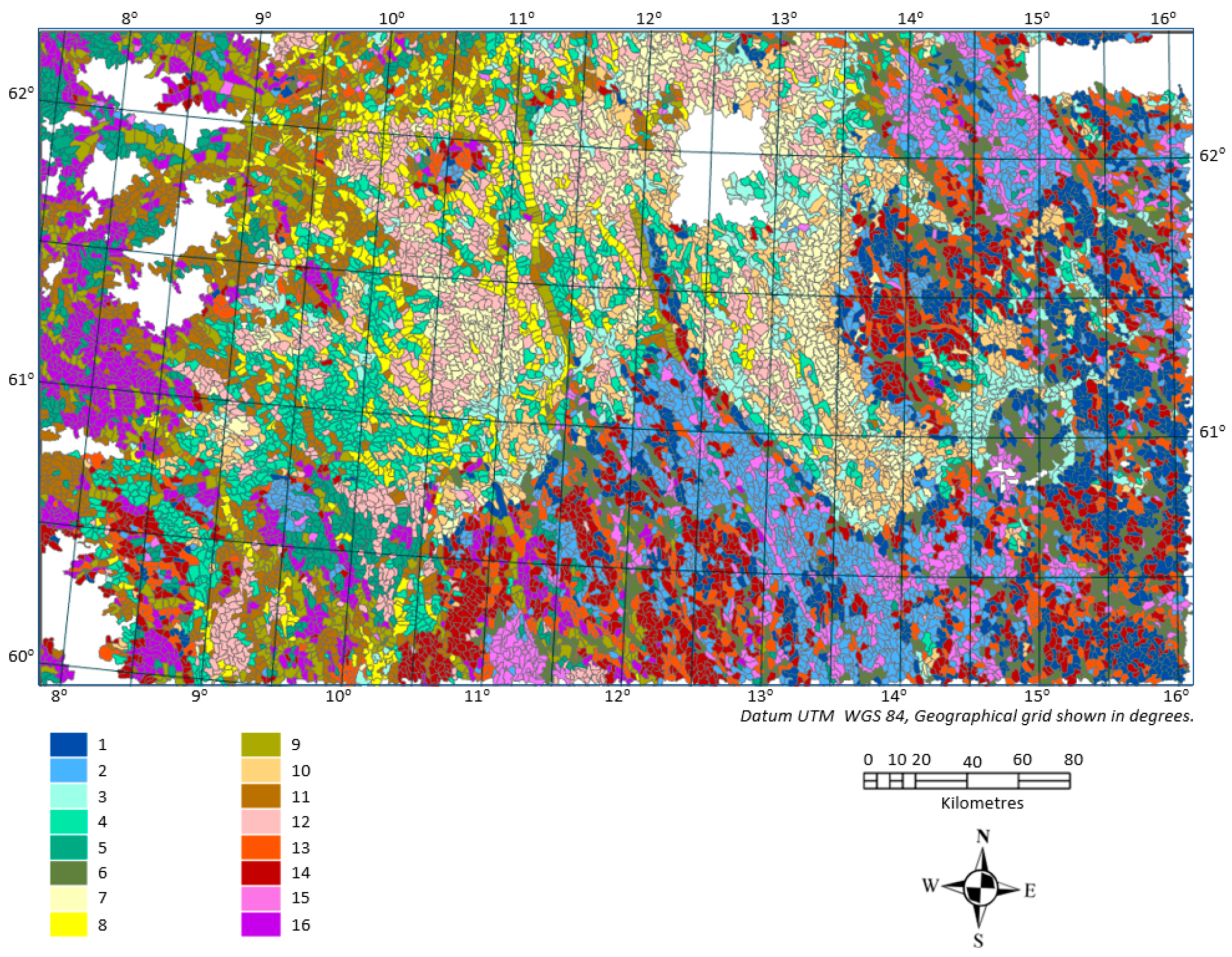
A visualised clustered PCA of all four axes is shown in Figure 7. We have chosen to show this variation as 16 clusters. Since the data were originally given as a stepless model along the four PCA axes, the results could be presented in several ways to illustrate the geographic distribution. The 16 clusters are a “random” number for the purpose of illustration but yield a recognisable pattern with a clear gradient from west to east, with cluster 5 and 15 dominating in the west and 1 and 3 in the east.
Each cluster contains 500–1300 landscape polygons. The clusters containing the most landscape polygons are numbers 14, 2 and 4, all with more than 1100 polygons. The smallest cluster is number 9 containing approximately 500 polygons.
To analyse the clusters in more detail compared with the PCA, we averaged the PC values in each cluster (see Appendix B). To further simplify the interpretation, we divided the PC scores into three groups: low = PC scores < −0.5, middle = PC scores −0.5 to 0.5, and high = PC scores > 0.5, indicated by the intensity of the shading in Table 3. To understand the colourised Table 3, one needs to translate the PC axes to the interpretations of the axes (see discussion of this above). For example, the first cluster has low PC1 values but high PC2 values, which most certainly means that the polygons in this cluster have flat terrain and contain sandstone. High PC3 and low PC4 values show that this cluster most certainly contains river deposits and has a low variation in rock diversity. In this way, it is possible to describe the 16 clusters with characteristics inferred from the analyses (PCA) in the study.
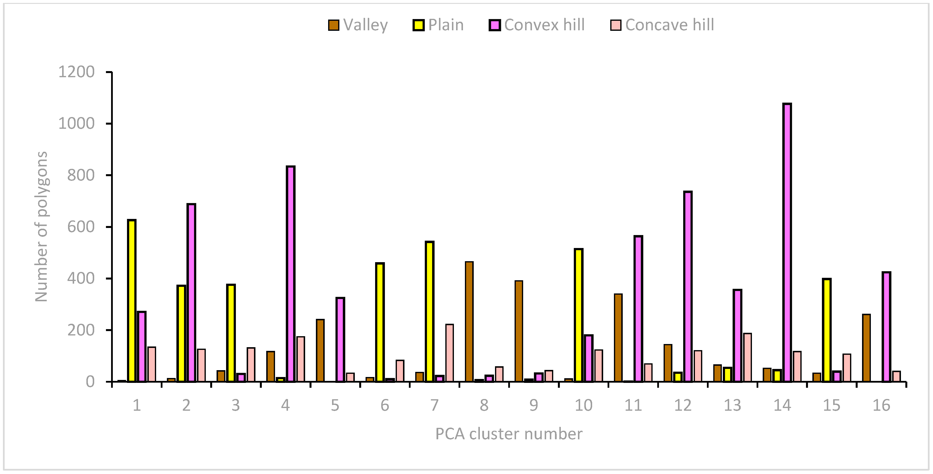
Table 3 can be regarded as a descriptive geodiversity model of the area with each cell containing a complex message given by the PCA results of the four axes. Since each of the landscape polygons also has attributes attached to them from the initial landscape type map, this division can be compared with the major landscape types originally defined in the landscape type map (Figure 3). In our analysis, we separated four different landscape types: valley landscapes, plains, hill and mountain landscapes in a convex setting, and hill and mountain landscapes in a concave setting. Because our new supplementary PCA analysis does not take this original division into account, and the first principal axis is highly influenced by terrain, these two perspectives will partly show elements of the same attributes. The best example is plains that per definition will fall within calm terrain. The relationship between the new PCA-based clusters and the landscape types is shown in Figure 8.
We can see from Figure 8 that plains have their maximum in clusters 1, 2, 3, 6, 7, 10 and 15, which all are interpreted as calm and flat terrain in Table 3. The valley landscape is, on the other hand, found in steep and rough terrains, which is expected as the definition for the valley landscape type requires a certain relief. It is, however, found to a lesser degree in cluster 4 than the other clusters interpreted as steep and rugged terrain in Table 3, and is also found in cluster 12 in medium steep terrain. The hill and mountain landscapes (convex hill) are represented in all three terrain groups, but peaks in the medium terrain class (cluster 14). Shallow valleys and depressions in the hill and mountain landscapes (concave hill) have lower frequency and are more evenly distributed among the terrain classes, but have a distinctly lower occurrence in the steep terrain, except in cluster 4.

4. Discussion

The multivariate analysis of the dataset yielded four very clear gradients. The first consists of topography, the second bedrock units, the third bedrock diversity (diversity of mapped bedrock units) and the fourth soil units. It was expected that there would be clear relationships between bedrock classes and terrain, but these relationships are weak. The four axes represent in a way four elements of geodiversity, with no strong relationships between them.
Some relationships are, however, visible. Bare rock and thin layer of till tend to be found in areas with steep terrain, and peat and thick till in flat terrain. Ultrabasic, basic, and intermediate metamorphic rock (amphibolite, eclogite, etc.) and partly ultrabasic, basic and intermediate intrusive rock including mafic dykes (gabbro, diorite, dolerite, etc.) are found on the steep terrain side of the gradient. These rocks are common in the Norwegian high mountains in the western part of the study area, which has steep terrain. This may be for several reasons, one of them being higher resistance to erosion on a local scale. However, this could also be a result of the general bedrock distribution and the regional geological history. Ultrabasic, basic and intermediate intrusive rock and acidic volcanic rock (rhyolite, dacite, etc.), rock diversity and amount of rock outcrops are found on the acidic intrusive rock (granite and granitic gneisses) side of axis number two, and carbonate-rich rock (limestone, dolomite, marble, etc.) on the quartz-feldspar-rich sedimentary rock (sandstone, greywacke, etc.) side of the axis. This illustrates a crystalline rock–sedimentary gradient. Interestingly, the frequency of cliffs measured on the 100 m DEM and the distance to steep terrain pull in the same direction, while cliffs measured on a 2 m resolution are neutral. This pattern seems contradictory as the first is normally associated with steep terrain and the other with flat terrain. The terrain in areas with sedimentary rocks may, however, be affected by the local structure geology conditions and contain both terrain types.
The rock diversity axis (third axis) shows that carbonate-rich rock, quartz-feldspar-rich sedimentary rock, and ultrabasic, basic and intermediate intrusive rock contribute mostly in the direction of high rock diversity, together with variables indicating flat terrain, while acidic intrusive rocks (granite and granitic gneisses) form more homogenous areas with less diversity. The fourth axis is mostly linked to soil and sediments. River sediments, glacifluvial sediments and aspects of soil diversity, such as fluvial and glacifluvial deposits normally found in valleys and depressions, form one end of the axis, together with flat terrain, thin till cover, scree and steep terrain forming the other. Both scree in steep terrain and sediments in flat terrain are normally sediment types that increase diversity, whereas thick and thin till cover and no sediment cover have a more even distribution. In the other direction are located thin till cover, peat, distance to steep terrain, terrain openness (and terrain position index values (TPI)). Alkaline rocks, basalt and gabbro pull moderately in the same direction. This picture is consistent with a soil diversity distribution where valleys and steep slopes with scree increase diversity and calm terrain in plains and low hills does not. In these landscapes large mires with peat are very common.
Analysing the overall result of the bedrock conditions and comparing these with the small test area (Figure 3), it seems like structural geology is the most important geological attribute linking bedrock with the terrain. This linkage is much more likely to illustrate the linkage between bedrock geology and terrain than using coarse-scale bedrock classes, at least at this scale, and with the specification that we have used. On a general level the 2 m-resolution terrain model picks up elements of structural geology through indices measuring terrain roughness such as the VRM index. However, if not geologically interpreted, it is difficult to assess if the relatively weak links between mapped bedrock classes can be explained by the lack of structural interpreted geological data, or if the bedrock classes are simply too generalised for this purpose. This may imply that even if such relationships can be observed in the field, they are not widespread enough to make a significant impact in a regional quantitative study. Manosso and Nóbrega [31] report that the highest rate of geodiversity is found in the most eroded reliefs. In their study, it is a connection between the erosion results producing clear signals between terrain and geology. However, their study is from Brazil, where the subaerial erosional timespan is very long. In our study area, all the land has undergone glacial erosion and has been affected by subaerial erosion after glaciation for only the past 10,000 years. Even the possibilities for cold-based ice [18] over relatively large areas and the related reduced glacial erosion will probably not change this general difference.
Our analyses lack a good data input of landforms. Landforms are important within geodiversity, but are not mapped with good enough aerial coverage to be included in our regional analysis. It is desirable that landform mapping is increased and that new innovative methods in terrain modelling and data integration are implemented to help cover this gap in mapped geodiversity elements.
Although the dataset does not result in strong signals of variation where terrain and geology together form coincident axes of geodiversity, the four identified gradients can be used to represent geodiversity using simple classifications and GIS overlay techniques, as shown in Figure 7. Such a map represents a valuable contribution to the understanding of geodiversity patterns in the area and serves as a good starting point for more detailed analysis involving manual methods and field work. It also represents possibilities to compare geodiversity characteristics over a large area and thus to be used scientifically, for management and for tourism.
The original landscape map [19,20] classification is based on landscape gradients containing physical, biological and human land use attributes. The delimitation of the landscape types and landscape areas, however, is based on geomorphic criteria and thus shows important structures related to geodiversity on a coarse scale. In this way the geodiversity can be analysed alone, but also in a wider landscape setting including both ecological and cultural aspects of the landscape.
The delimitation is based on a course elevation model (100 m resolution interpolated from 20 m contour lines) and lacks detailed terrain structures, which have recently become accessible with new LiDAR datasets and derived detailed terrain models. When linking these new datasets to the original information base, it will be possible to mitigate other limitations in the existing available data sets. Landforms can then be mapped more efficiently and they can be modelled to contribute to more accurate and less biased maps, and even better models of structural geology seem to be within reach.
For this study, however, such datasets were not yet available, and we had to perform the analysis with more traditional data input, i.e., geological maps at a scale of 1:250,000 and quaternary geology maps of similar scale. However, we managed to put together terrain data that also included 10 m and 2 m terrain models based on LiDAR. There are more detailed geological maps, but the coverage is still too low to offer sufficient data input covering the entire study area. Even within our rather robust sampling strategy, there are areas with no data in the dataset that affect the coverage of good analytical results. There is still a lack of detailed (2 m resolution) LiDAR data in some western mountainous areas of Norway, and the quaternary geology maps from Sweden are not available for some areas. Areas suffering these data limitations were excluded in the analysis as they produce artifacts that become visible in the third and fourth PCA axes calculated. Moreover, the quaternary geology database of Norway has inputs from different scales that may introduce a bias that is not easily controlled. These issues are important limitations for all geodiversity analysis [12] as they represent fundamental data input. What is measured or assessed here is not the in situ detailed elements of geodiversity, but the mapped elements of geodiversity as it appears on maps and in databases that are available to us. In smaller areas, this issue can be solved by intensive field work, but in regional studies this will not be possible.
Forte et al. [8] points out that this issue also causes problems when comparing areas and regions if the data input for these regions do not use the same classification system. In this study, this problem led to the need to homogenise the geological maps on the coarsest specification level and even combine classes of bedrock into more general classes because the classification systems in Sweden and Norway are different. The homogenisation and simplification solve the problem of comparing data, but the process results in data loss concerning important information on geodiversity.

5. Conclusions

The multivariate analysis identified four major geodiversity gradients. These gradients are related to terrain variation, bedrock units, bedrock diversity and soil/sediments distribution. They make it possible to map a geodiversity profile for landscape type areas over a large region.
The main uncertainties in the analysis are linked to a lack of data describing the geographical distribution of landforms and structural geology and the generalisation level of geological units, and the generally course scale of geological input.
The multivariate analysis does not show strong links between terrain structures and geological units, maybe because they have been mapped at a scale of 1:250,000. The expected signals between bedrock types and terrain measured at detailed scales have not been detected clearly; however, some relationships are visible in the analytical results. These signals are interpreted as descriptive relationships and not as casual effects. The data and extent of the study area are hardly large enough to draw firm conclusions, but more detailed investigations into the results may make it possible to build some hypotheses that later can be tested.
Manual inspection of the terrain data shows that terrain ruggedness is generated most of all by structural geological features that are not necessarily linked to the bedrock classes on the generalisation level we have used in this study. The study area has a short history of subaerial erosion, thus these processes have not had enough time to mature.
Together with the information collected from the already existing landscape type map, the procedure provides the opportunity to make analytical maps through simple overlay techniques and to compare areas with each other with respect to their geodiversity profile. This can be carried out both alone and in a wider landscape setting. The obtained results will also serve as a digital basis to be supplemented with more detailed data as they become available, including data from studies involving manual mapping methods and field work.

Author Contributions

Conceptualization, L.E., V.B. and T.L.A.; data curation, L.E., M.L.A. and A.M.; formal analysis, L.E. and V.B.; funding acquisition, R.D. and L.W.; investigation, L.E., M.L.A., A.M., T.L.A. and L.W.; methodology, L.E. and V.B.; project administration, L.E., R.D., T.L.A. and L.W.; writing—original draft, L.E.; writing—review & editing, L.E., V.B., R.D., M.L.A. and A.M. All authors have read and agreed to the published version of the manuscript.

Funding

This article is written as part of the GNIST project (Geological heritage in Nature-based Innovation for Scandinavian Tourism), funded by grants from the Interreg Sweden–Norway programme 2014–2020 Inner Scandinavia, under the priority: Innovative Environments (ref. application no. 2019-0021, archive no. 2020/28924), as well as the Regional Development Fund of Innlandet county (Norway) (same reference as Interreg) and the project partners (NGU, SGU, NINA, Norske Parker, and Region Dalarna). We have also received strategic funding for NINA from The Research Council of Norway, project no. 160022/F40.

Institutional Review Board Statement

Not applicable.

Informed Consent Statement

Not applicable.

Data Availability Statement

The data presented in this study are available on request from the corresponding author. The data are not publicly available due to lack of host and size of GIS-files.

Acknowledgments

We wish to thank our institutions, partners and funders in the GNIST project for enabling us to perform the work described in the article. We would also like to express our gratitude to our Swedish partners in The Geological Survey of Sweden for data deliverance and fruitful discussions; in particular, Gunnel Ransed and Kristian Schoning.

Conflicts of Interest

The authors declare no conflict of interest.

Appendix A

R-script for PCA analysis:
pca10 <- read.table (“clipboard”, header = T)
attach (pca10)
names (pca10)
library (vegan)
pca10pca <- rda (pca10, scaling = 1, axes = 8, scale = T)
pca10pca
summary (pca10pca, axes = 0)
scores (pca10pca, choices = c (1,2), display = c (“sp”))
pcas <- scores (pca10pca, choices = c (2), display = c (“sites”))
plot.cca (pca10pca)
sitescores <- scores (pca10pca, choices = c (1,2), display = c (“si”))
write (sitescores, file = “c:/PCA/pca10r1.txt”, ncolumns = 1)
plot.cca (pca10pca, type = “n”)

Appendix B

Mean PCA values for the 16 clusters shown in Figure 7 and Table 3.
Cluster IDCount of Cluster IDAverage of PC1Average of PC2Average of PC3Average of PC4
11035−0.8980.8990.633−0.656
21198−0.5610.480−1.564−0.538
3579−0.983−0.6301.2341.078
411390.600−0.7430.925−0.725
56001.0030.077−1.7390.132
6568−1.1251.0220.6071.387
7922−1.151−1.623−0.591−0.033
85510.802−0.9940.4431.780
94801.0920.4840.3071.948
10828−0.842−0.7461.141−0.575
119751.313−0.1990.472−0.028
1210350.442−1.313−0.962−0.536
13662−0.0401.0740.4230.365
1412910.2071.0590.378−0.958
15577−1.1610.528−1.4311.332
167281.3850.932−0.0690.080

References

  1. Gray, M. Geodiversity: Valuing and Conserving Abiotic Nature, 2nd ed.; Wiley Blackwell: Chichester, UK, 2013; 495p. [Google Scholar]
  2. Australian Heritage Commission. Australian Natural Heritage Charter, 2nd ed.; Australian Heritage Commission: Canberra, Australia, 2002; 26p.
  3. Johansson, C. Geodiversitet i Nordisk Naturvård; Nordisk Ministerråd: Copenhagen, Denmark, 2000; 149p. [Google Scholar]
  4. Noss, R.F. Indicators for monitoring biodiversity: A hierarchical approach. Biol. Conserv. 1990, 4, 355–364. [Google Scholar] [CrossRef]
  5. Chiarucci, A.; Bacaro, G.; Scheiner, S.M. Old and new challenges in using species diversity for assessing biodiversity. Philos. Trans. R. Soc. Lond. B Biol. Sci. 2011, 366, 2426–2437. [Google Scholar] [CrossRef] [PubMed] [Green Version]
  6. Gray, C.; Hill, S.; Newbold, T.; Hudson, L.N.; Börger, L.; Contu, S.; Hoskins, A.J.; Ferrier, S.; Purvis, A.; Scharlemann, J.P.W. Local biodiversity is higher inside than outside terrestrial protected areas worldwide. Nat. Commun. 2016, 7, 12306. [Google Scholar] [CrossRef] [PubMed] [Green Version]
  7. Forte, J.P.; Brilha, J.; Pereira, D.Í.; Nolasco, M. Kernel density applied to the quantitative assessment of geodiversity. Geoheritage 2018, 10, 205–217. [Google Scholar] [CrossRef] [Green Version]
  8. Supriatna, J. Biodiversity Indexes: Value and evaluation purposes. Web Conf. 2018, 48, 01001. [Google Scholar] [CrossRef]
  9. Morris, E.K.; Caruso, T.; Buscot, F.; Fischer, M.; Hancock, C.; Maier, T.S.; Meiners, T.; Müller, C.; Obermaier, E.; Prati, D.; et al. Choosing and using diversity indices: Insights for ecological applications from the German biodiversity exploratories. Ecol. Evol. 2014, 4, 3514–3524. [Google Scholar] [CrossRef] [PubMed] [Green Version]
  10. Serrano, E.; Ruiz-Flano, P. Geodiversity: A theoretical and applied concept. Geogr. Helv. 2007, 62, 140–147. [Google Scholar] [CrossRef]
  11. Hjort, J.; Luoto, M. Geodiversity of high-latitude landscapes in northern Finland. Geomorphology 2010, 115, 109–116. [Google Scholar] [CrossRef]
  12. Pereira, D.; Pereira, P.; Brilha, J.; Santos, L. Geodiversity assessment of Paraná state (Brazil): An innovative approach. Environ. Manag. 2013, 52, 541–552. [Google Scholar] [CrossRef] [PubMed] [Green Version]
  13. Araujo, A.M.; Pereira, D. A New Methodological Contribution for the Geodiversity Assessment: Applicability to Ceará State (Brazil). Geoheritage 2017, 10, 591–605. [Google Scholar] [CrossRef]
  14. Koistinen, T.; Stephens, M.B.; Bogatchev, V.; Nordgulen, Ø.; Wennerstrøm, M.; Korhonen, J. Geological map of the Fennoscandian Shield, scale 1:2 million. In Geological Surveys of Finland, Norway and Sweden and the North-West Department of Natural Resources of Russia; Genimap Oy: Helsinki, Finland, 2001. [Google Scholar]
  15. Ramberg, I.; Bryhni, I.; Nøttvedt, A.; Rangnes, K. The Making of a Land. Geology of Norway; Norsk Geologisk Forening: Trondheim, Norway, 2008; 624p. [Google Scholar]
  16. Stroeven, A.P.; Hättestrand, C.; Kleman, J.; Heyman, J.; Fabel, D.; Fredin, O.; Goodfellow, B.W.; Harbor, J.M.; Jansen, J.D.; Olsen, L.; et al. Deglaciation of Fennoscandia, Quat. Sci. Rev. 2016, 147, 91–121. [Google Scholar] [CrossRef] [Green Version]
  17. Stephens, M.B.; Weihed, J.B. Sweden: Lithotectonic framework. Tectonic Evolution and Mineral Resources. Geol. Soc. Lond. Mem. 2020, 50, 253–268. [Google Scholar] [CrossRef] [Green Version]
  18. Olsen, L.; Fredin, O.; Olesen, O. Quaternary Geology of Norway-Geological Survey of Norway Special Publication 13; Geological Survey of Norway: Trondheim, Norway, 2013; 173p. [Google Scholar]
  19. Halvorsen, R.; Skarpaas, O.; Bryn, A.; Bratli, H.; Erikstad, L.; Simensen, T.; Lieungh, E. Towards a systematics of ecodiversity: The ecosyst framework. Glob. Ecol. 2020, 29, 1887–1906. [Google Scholar] [CrossRef]
  20. Simensen, T.; Erikstad, L.; Halvorsen, R. Diversity and distribution of landscape types in Norway. Norsk Geog. Tidsskr. 2021, 75, 79–100. [Google Scholar] [CrossRef]
  21. Simensen, T.; Halvorsen, R.; Erikstad, L. Gradient analysis of landscape variation in Norway. bioRxiv 2020, 161372. [Google Scholar] [CrossRef]
  22. Gruber, S.; Peckham, S. Land-surface parameters and objects in hydrology. In Geomorphometry: Concepts, Software, Applications; Hengl, T., Reuter, H.I., Eds.; Elsevier: Amsterdam, The Netherlands, 2008; pp. 171–194. [Google Scholar]
  23. Riley, S.J.; DeGloria, S.D.; Elliot, R. A terrain ruggedness index that quantifies topographic heterogeneity. Intermt. J. Sci. 1999, 5, 23–27. [Google Scholar]
  24. Sappington, J.M.; Longshore, K.M.; Thompson, D.B. Quantifying landscape ruggedness for animal habitat analysis: A case study using bighorn sheep in the Mojave Desert. J. Wildl. Manag. 2007, 71, 1419–1426. [Google Scholar] [CrossRef]
  25. Jenness, J. Topographic Position Index (tpi_jen.avx) Extension for ArcView 3.x, v. 1. Jenness Enterprises. Available online: http://www.jennessent.com/arcview/tpi.htm (accessed on 20 May 2022).
  26. Conrad, O. SAGA-GIS Module Library Documentation (v2.2.5). Available online: https://saga-gis.sourceforge.io/saga_tool_doc/2.2.5/ta_lighting_5.html (accessed on 20 May 2022).
  27. Sokal, R.R.; Rohlf, F.J. Biometry: The Principles and Practice of Statistics in Biological Research, 3rd ed.; Freeman: New York, NY, USA, 1995; 887p. [Google Scholar]
  28. Økland, R.H.; Økland, T.; Rydgren, K. Vegetation–environment relationships of boreal spruce swamp forests in Østmarka nature reserve, SE Norway. Sommerfeltia 2001, 29, 1. [Google Scholar] [CrossRef]
  29. Braak, C.J.F.T. Canonical correspondence analysis: A new eigenvector technique for multivariate direct gradient analysis. Ecology 1986, 67, 1167–1179. [Google Scholar] [CrossRef] [Green Version]
  30. Oksanen, J.; Guillaume Blanchet, F.; Friendly, M.; Kindt, R.; Legendre, P.; McGlinn, D.; Minchin, P.R.; O’Hara, R.B.; Simpson, G.L.; Solymos, P.; et al. Vegan: Community Ecology Package, Ver. 2.5-7. Available online: http://cran.r-project.org (accessed on 11 April 2022).
  31. Manosso, F.C.; de Nóbrega, M.T. Calculation of geodiversity from landscape units of the cadeado range region in Paraná, Brazil. Geoheritage 2016, 8, 189–199. [Google Scholar] [CrossRef]
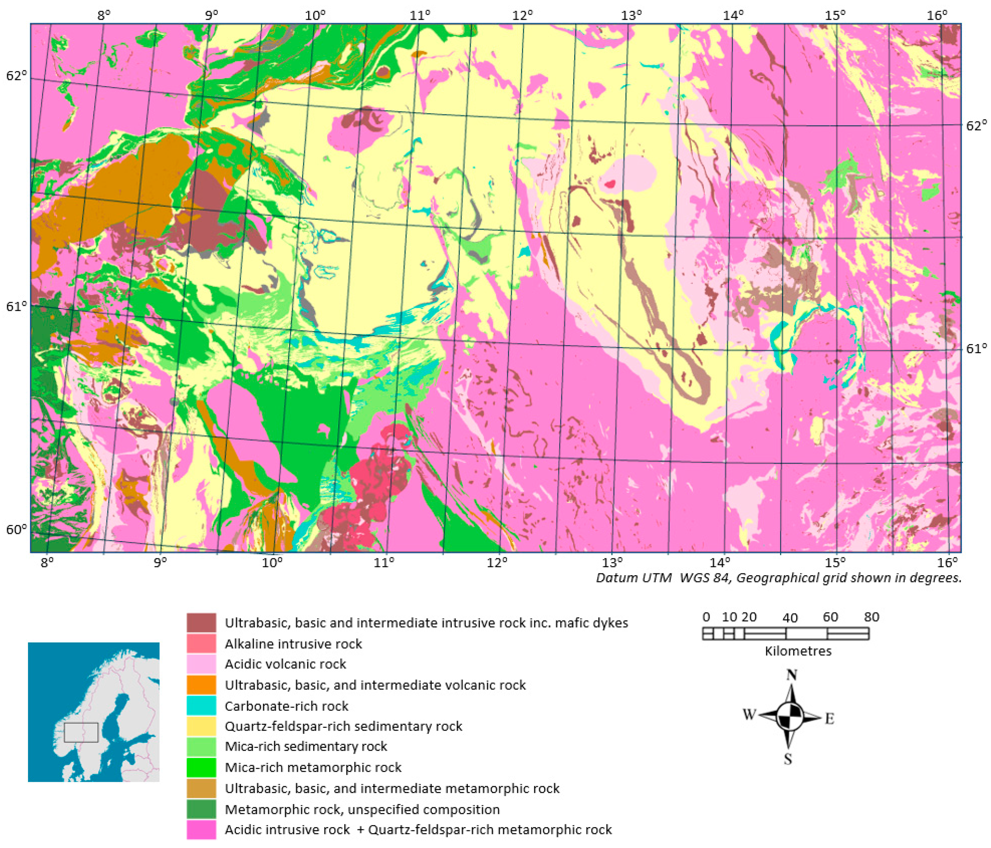
Figure 1. Bedrock map of the area. The map is put together through a homogenisation and simplification of geological maps from Swedish and Norwegian bedrock databases (www.sgu.se, www.ngu.no (accessed on 20 May 2022)) at a scale of 1: 250,000 with emphasis on the major rock classification. Several bedrock classes are combined, and the difference in classification systems between Norway and Sweden has made it necessary to only use regional data, introducing the risk of potential data loss.
Resources 11 00051 g001
Figure 2. Simplified Quaternary geology map of the area. The map was put together by homogenising and simplifying Quaternary geology maps from Swedish and Norwegian databases of quaternary deposits (www.sgu.se, www.ngu.no (accessed on 20 May 2022)) at a scale of 1:250,000. A difference in classification systems and the resulting simplification and use of regional data may lead to data loss for some important geological features.
Resources 11 00051 g002
Figure 3. The landscape areas of the study area classified by which major landscape type they belong to. A small area used for testing the detailed representation of terrain ruggedness (Figure 4) is situated within the red circle in the map.
Resources 11 00051 g003
Figure 4. Hill shade map for the test area in Lalm with a resolution of 1 m based on Lidar measurements, Vågå municipality (for location see Figure 3). The different characteristics assessed are: (A) Glacifluvial deposits in the form of terraces and chute eskers linked to glacial directed drainage from the neighbouring valley. Relatively course scale, but very distinct slopes; (B) Rock fall scar in steep terrain on the upper part of the valley side, rugged on a fine scale; (C) Cliffs in the upper valley side. Rugged on a course scale and very steep; (D) Bedrock structures due to layered rocks (slates) cutting the surface in a steep angle, visible terrain ruggedness in a medium scale; (E) As (D), but in phylittic rocks; (F) Erosional features in the soils filling the lower part of the valley side, terrain ruggedness in a fine scale; (G) flat areas representing river surface and anthropogenic structures like football fields and industrial facilities; (H) Bedrock structures due to layered rocks cutting the surface in a steep angle in phylittic rocks, visible terrain ruggedness in a fine scale; (I) The same, but slightly coarser scale accentuated by small quarries. Note that this is a very detailed study within parts of very few landscape areas. LiDAR data on this resolution are influenced by both small and larger man-made objects such as roads, dams, and other infrastructure and terrain modifications.
Resources 11 00051 g004
Figure 5. The first and second axis of the multivariate analysis with loadings for the different variables in the ordination diagram. Bedrock variables are shown in green squares, Quaternary deposit variables are represented by red dots and terrain variables are shown as blue triangles. The first axis, explaining 28.7% of the total variation, sorts out variables along a gradient reflecting the topography going from lands dominated by steep terrain and high ruggedness having high values, to variables associated with smooth landscapes showing low values along axis 1. The second axis, explaining an additional 13.5% of the total variation, span a gradient heavily influenced by geology. On high loadings we find quartz- and feldspar-rich sedimentary rocks (Quartz_sed) while ultrabasic, basic and intermediate intrusive rocks such as gabbro, acidic volcanic rock such as granite/granitic gneisses with migmatite (Basic_intr), thin till cover (Thin till) and bedrock diversity (Rock div) pull in the other direction.
Resources 11 00051 g005
Figure 6. The third and fourth axis of the multivariate analysis with loadings for the different variables in the ordination diagram. Bedrock variables are shown in green squares, Quaternary deposits variables are represented by red dots and terrain variables are shown as blue triangles. Rock type diversity (Rock div) shows the highest values along the third axis with ultrabasic, basic and intermediate intrusive rocks (Basic_intr) on the opposite end of the axis. Additionally, acidic volcanic rocks (Acid_intr) have high negative loadings along this axis.
Resources 11 00051 g006
Figure 7. The results of the PCA analysis shown as landscape area values in 16 clusters.
Resources 11 00051 g007
Figure 8. Number of landscape areas within each PCA cluster (Figure 7) relative to landscape types.
Resources 11 00051 g008
Table 1. A visual assessment of the response of different indices in the test areas defined in the text above and in Figure 4. -: no response, X: weak, XX: fairly strong and XXX: strong.
1 m Resolution10 m Resolution
Plancurv.Aspectdiv.Rough/TRIVRMAspectdiv.VRM
AXXXXXXXXX
BXXXXXXXX--
CXXXXXXXXXXXXXX
D-XXX-XXXXX-
E-XX-XX--
FXXXXXX--
G-XXX--XX-
HXXXXXXXXXXX-
IXXXXXXXXXXX-
Table 2. Variables used for the analysis in the test area.
Variable DescriptionShort NameMeasure Units
Bedrock units:
Ultrabasic, basic and intermediate intrusive rock inc. mafic dykes (gabbro, diorite, dolerite, etc.)
Basic_intrCoverage
(mean number of cells relative to number of cells in the polygon)
Alkaline intrusive rockAlkaline_intr
Acidic volcanic rock (rhyolite, dacite, etc.)Acidic_volc
Ultrabasic, basic, and intermediate volcanic rock (basalt, andesite, etc.)Basic_volc
Carbonate-rich rock (limestone, dolomite, marble, etc.)Carbonate
Quartz-feldspar-rich sedimentary rock (sandstone, greywacke, etc.)Quartz_sed
Mica-rich sedimentary rock (shale, siltstone, etc.)Mica_sed
Mica-rich metamorphic rock (phyllite, schist, paragneiss, etc.)Mica_met
Ultrabasic, basic, and intermediate metamorphic rock (amphibolite, eclogite, etc.)Basic_met
Metamorphic rock, unspecified composition (diatexitic migmatite, mylonite, granofels, etc.)Unspecified_met
Acidic intrusive rock (granite, granodiorite, monzonite, etc.) + Quartz-feldspar-rich metamorphic rock (gneiss, granitic gneiss, etc.)Acidic_intr
Rock type diversityRock div.
Soil and water:
Water (lakes and broad rivers)
Water
PeatPeat
Bare rockBare
Continous till coverTill
FluvialdepositsFluvial
Thin till coverThin till
Glaciofluvial deposits?Glaciofluvial
Scree depositsScree
Weathering bedrockWeathering
Anthropogenic materialAnthropogenic
Glaciolacustrine depositsGlacilac
Beach depositsBeach
Fiord- and sea depositsFiord/sea deposits
Aeolian sedimentsAeolian
Clayey tillClay
Soil deposit diversitySoil diversity
Terrain indices and measurements:
Relative relieff 100 m resolution
RR100Elevation range in metres
Terrain position index [25] values (TPI) larger than 15 m at 100 m resolutionTPI100Coverage
Distance to TPI values larger than 15 m at 100 m resolutionDistTPI100Mean distance in metres
Vector ruggedness values at 100 m resolutionVRM100Mean values
Number of pixels with slope values larger than 30 degrees Cliff100Coverage
Positive openess [26]PosopenMean value
Relative relief 10 m resolution on a local scaleRR10Mean value of elevation range in metres in circles with diameter 10 cells.
Flat (<2-degree slope) at 10 m resolutionFlat10Coverage
Steep (>30-degree slope) at 10 m resolutionSteep10
Distance to Steep (>30-degree slope) at 10 m resolutionDistSteep10Mean value
Slope at 10 m resolutionSlope10
Cliffs (>38-degree slope) at 2 m resolutionCliff2Coverage
Steep (>30-degree slope) at 2 m resolutionSteep2
Flat (<2-degree slope) at 2 m resolutionFlat2
Distance to Steep (>30-degree slope) at 2 m resolutionDistFlat2
Vector ruggedness values at 100 m resolutionVRM2Mean value
Table 3. Interpretation of the PCA results (Table 3) for the 16 clusters shown in Figure 7. The colour indicates the level of PCA values, low (lightest), middle and high values (darkest).
Cluster IDInterpretation of PC1Interpretation of PC2Interpretation of PC3Interpretation of PC4
1Calm and flat terrainSandstone dominationHigh bedrock diversityDominated by moraine
2Calm and flat terrainIntermixed sedimentary and eruptiveLow bedrock diversityDominated by moraine
3Calm and flat terrainGneiss and granite dominationHigh bedrock diversityHigh amount of river deposits
4Rough and steep terrainGneiss and granite dominationHigh bedrock diversityDominated by moraine
5Rough and steep terrainIntermixed sedimentary and eruptiveLow bedrock diversityIntermixed river deposits and moraine
6Calm and flat terrainSandstone dominationHigh bedrock diversityHigh amount of river deposits
7Calm and flat terrainGneiss and granite dominationLow bedrock diversityIntermixed river deposits and moraine
8Rough and steep terrainGneiss and granite dominationMedium bedrock diversityHigh amount of river deposits
9Rough and steep terrainIntermixed sedimentary and eruptiveMedium bedrock diversityHigh amount of river deposits
10Calm and flat terrainGneiss and granite dominationHigh bedrock diversityDominated by moraine
11Rough and steep terrainIntermixed sedimentary and eruptiveMedium bedrock diversityIntermixed river deposits and moraine
12Median steep and undulating terrainGneiss and granite dominationLow bedrock diversityDominated by moraine
13Median steep and undulating terrainSandstone dominationMedium bedrock diversityIntermixed river deposits and moraine
14Median steep and undulating terrainSandstone dominationMedium bedrock diversityDominated by moraine
15Calm and flat terrainSandstone dominationLow bedrock diversityHigh amount of river deposits
16Rough and steep terrainSandstone dominationMedium bedrock diversityIntermixed river deposits and moraine
Publisher’s Note: MDPI stays neutral with regard to jurisdictional claims in published maps and institutional affiliations.