Abstract
The frequency characteristics of the switching-mode power supply (SMPS) control loop under all operating conditions are crucial for performance evaluation and defect detection. Traditional methods, relyingon experiments under preset conditions, struggle to achieve comprehensive evaluation. This study proposes a frequency characteristic fitting method for all operating conditions based on FT-WOA-MLP. A discrete-point dataset covering all conditions of an LLC SMPS was obtained using the small-signal perturbation method, including input voltage, output current, injection frequency, and corresponding amplitude- and phase-frequency characteristics. The multilayer perceptron (MLP) model was trained on the training set covering all operating conditions, with the whale optimization algorithm (WOA) used to optimize the learning rate, and fine tuning (FT) applied to further enhance accuracy. Independent test set validation showed that, for amplitude-frequency characteristics, the mean absolute error (MAE) was 2.0995, the mean absolute percentage error (MAPE) was 0.0974, the root mean square error (RMSE) was 4.0474, and the coefficient of determination (R2) reached 0.92; for phase-frequency characteristics, the MAE was 3.502, the MAPE was 0.0956, the RMSE was 10.5192, and the R2 reached 0.94. The method accurately fits frequency characteristics under all conditions, supporting defect identification and performance optimization.
1. Introduction
The application of new materials such as silicon carbide (SiC) and gallium nitride (GaN) has significantly improved the power density and conversion efficiency of switching-mode power supply (SMPS). The coordinated application of its high-frequency technology and digital control technology has achieved volume and weight reduction, efficiency optimization, and intelligent, networked, and modular functional integration while ensuring system stability and reliability [1,2,3,4]. The SMPS has been widely used in important fields such as industrial equipment, transportation, and medical devices [5,6,7].
At present, the SMPS control loop is mainly tested by injecting interference signal sweep frequency for frequency characteristic analysis [8]. The dynamic performance and reliability verification of its control loop relies heavily on the accumulation of experimental data, and the debugging effect of the control loop parameters is greatly affected by the subjective engineering experience of technicians. This leads to inconsistent debugging outcomes, negatively impacting the uniformity of product performance and hindering the pace of product iteration. In view of the above problems, it is urgent to study the frequency characteristic fitting method of the SMPS control loop under all operating conditions to provide technical support for identifying potential defects and optimizing performance under all operating conditions.
Currently, commonly used fitting methods include interpolation, function fitting, regression analysis, and artificial intelligence (AI) methods [9,10,11,12]. The AI (machine learning) fitting method can overcome limitations inherent in interpolation, function fitting, and regression analysis, such as complex independent modeling for each operating condition, inadequate representation of nonlinear relationships, and burdensome repetitive experiments. Consequently, it has emerged as a research focus for characteristic fitting applications [13].
In the field of characteristic fitting, AI algorithms such as long short-term memory networks (LSTM), convolutional neural networks (CNNs), and multilayer perceptron (MLP) have been widely used in model construction and prediction [14,15,16,17]. In recent years, MLP has attracted widespread attention from scholars worldwide for its advantages such as nonlinear fitting capability and multi-level structure. For example, Reference [18] utilized the deep hierarchical structure of MLP to explicitly characterize nonlinear characteristics of hardware, exposing bottlenecks of line resistance, thereby promoting the optimization design of MCA structure. This work aims to develop a fast and comprehensive surrogate covering the full operating domain of the LLC converter, which provides closed-loop frequency responses for stability evaluation, parameter trade-off studies, and component what-if analyses. The choice of MLP is motivated by its ability to provide the following:
- Deployability: small parameter count and low inference latency (embedded/edge friendly).
- Data fit: stable, reproducible training on modest FRA datasets (144 × 81).
- Continuity: a smooth frequency-response “surface” over the operating domain, unlike per-point models.
- Complementarity: analytical baselines (FHA/refined average) give physical intuition; the MLP supplies high-fidelity, cross-condition fitting and instant querying.
In addition, model parameters are often affected by human subjective factors such as engineering experience in the modeling process. This can result in reduced model generalization, as well as issues like overfitting or underfitting caused by the use of empirical parameters. Swarm-based optimization methods, such as particle swarm optimization (PSO), the genetic algorithm (GA), and the whale optimization algorithm (WOA), have been successfully applied in the optimization of control parameters of nonlinear systems. Notably, the WOA exhibits more powerful search capability for global optimal solution [19,20,21,22]. Reference [23] proposed an EWOA-TPID controller with the WOA as the core to automatically optimize PID parameters, which significantly improved the dynamic performance of the model and demonstrated the convergence speed, global search, and local optimization advantages of the WOA. Reference [24] proposed to use the WOA to accurately tune the initial solution of the nonlinear equation in the harmonic elimination process, which significantly reduced the total harmonic distortion (THD), and the THD optimized by the WOA was 3.96% lower than that of other algorithms.
For established models, poor fitting accuracy often arises from varying operating conditions and data perturbations, necessitating systematic model refinement. As the core technology of transfer learning (TL), model fine-tuning (FT) has the advantage of realizing transfer learning of models with low data requirements by reusing pre-trained knowledge. It has been used for optimization and adjustment of models in terms of improving model accuracy and fault diagnosis [25,26,27]. In Reference [28], the DL model was fine-tuned using a small amount of real labeled data from the target domain through FT, enabling the DL model to adapt to the characteristic distribution of the target domain and completing the cross-domain work of the model under the premise of ensuring performance. Based on the above analysis of the advantages and applications of FT, it can be used for fine-tuning optimization of the MLP SMPS frequency characteristic fitting model.
In summary, this paper proposes a frequency characteristic fitting method of SMPS under all operating conditions based on an FT-WOA-MLP model to achieve good expected results in monitoring the trend of SMPS frequency characteristics with voltage and current changes under complete and continuous conditions. The structure of this paper is as follows: Section 2 summarizes the SMPS, the research object of this paper; Section 3 shows the modeling process of the proposed FT-WOA-MLP model; Section 4 describes the collection of frequency characteristic data through experiments, fits the data with the model, and analyzes the fitting results and accuracy; and Section 5 presents the conclusions of the study.
2. LLC SMPS and Its Frequency Characteristics
2.1. LLC SMPS
LLC stands for Inductor–Inductor–Capacitor resonant converter. Power switches Q1 and Q2 form a half-bridge inverter circuit. The resonant capacitor Cr, resonant inductor Lr and excitation inductor Lm constitute the resonant network. The center tap transformer (with a transformation ratio of n:1:1) and diodes D1 and D2 form a full-wave rectifier circuit. C0 is an output filter capacitor, and R0 is an output resistor. The circuit structure of the LLC SMPS is shown in Figure 1.
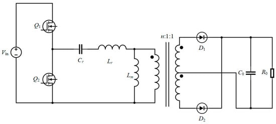
Figure 1.
LLC SMPS.
In Figure 1, denotes the DC input voltage. When the excitation inductor Lm is clamped by the output voltage through a transformer, Lm ceases to participate in resonance. The resonant frequency generated by the resonant inductor Lr and the resonant capacitor Cr is called the series resonant frequency (commonly abbreviated as resonant frequency). The resonant frequency fr is expressed as Formula (1):
When the primary and secondary sides of the transformer are disconnected, the excitation inductor Lm is no longer clamped by the output voltage, and the excitation inductor Lm, the resonant inductor Lr, and the resonant capacitor Cr resonate together. The generated resonant frequency is called the series–parallel resonant frequency (fm), which is expressed as Formula (2):
According to the relationship between the switching frequency f and the resonant frequencies fr and fm, there are three working modes of the LLC resonant converter:
- Working mode 1: f > fr, under-resonance mode.
- Working mode 2: f = fr, complete resonance.
- Working mode 3: fm < f < fr, quasi-resonant mode.
2.2. Frequency Characteristics of Control Loop
The training dataset is obtained entirely from experimental measurements using frequency response analysis (FRA) on the physical LLC prototype.
In this study, the system frequency characteristics are defined as how the output signal changes relative to the input signal as a function of the input signal frequency under steady-state conditions. These characteristics consist of the amplitude-frequency and phase-frequency responses, which can be obtained using the small-signal perturbation method and a loop tester. The test block diagram for frequency characteristics of the control loop is shown in Figure 2.
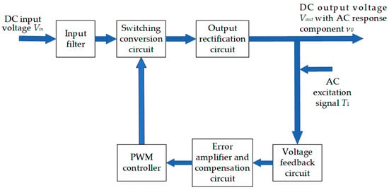
Figure 2.
Test block diagram for frequency characteristics of the control loop.
As shown in Figure 2 (test block diagram for frequency characteristics of the control loop), the LLC input is a DC voltage . A frequency-swept sinusoidal AC excitation signal is injected into the voltage feedback path, superimposed on the feedback voltage. The perturbed signal passes through the error amplifier and compensation circuit, and is then fed into the PWM controller, which modulates the switching frequency of the half-bridge inverter. Thus, the injected perturbation propagates through the power stage, and the output voltage exhibits an additional AC response component of superimposed on the original DC output . Measuring allows the loop gain and phase characteristics of the LLC SMPS to be derived.
The error amplifier and compensation circuit compare the sensed output voltage with the reference and provide frequency-domain shaping (pole–zero placement) to ensure sufficient phase margin and gain characteristics. In other words, the compensation circuit guarantees loop stability and dynamic performance. The PWM controller is still required because it converts the compensated error signal into a control action for the power stage, typically by adjusting the switching frequency in the LLC resonant converter. The compensation alone cannot directly drive the MOSFETs; the PWM controller interprets the compensated control signal and generates the gate pulses for the power switches. Therefore, both blocks are essential: compensation for shaping the loop dynamics, and the PWM controller for producing the switching action.
The amplitude-frequency characteristics and phase-frequency characteristics together constitute the frequency characteristics of the LLC SMPS.
- Amplitude-frequency characteristics: The amplitude ratio between the output AC response component and the input excitation signal T1 varies with frequency, usually expressed in decibels (dB). It reflects the system’s ability to amplify or attenuate signals of different frequencies. The magnitude is calculated using Formula (3):
- Phase-frequency characteristics: The phase difference between the output AC response component and the input excitation signal T1 varies with frequency, usually expressed in degrees (°) or radians (rad). It reflects the system’s ability to delay signals of different frequencies. The phase is calculated using Formula (4):
3. Establishment of Fitting Model
3.1. MLP Fitting Model
The multilayer perceptron (MLP) is a type of feedforward artificial neural network composed of an input layer, an output layer, and at least one hidden layer. Neurons between layers are fully connected through weight coefficients, and information is transmitted from the input layer to the output layer through the hidden layer.
The input layer receives external data. The number of nodes is determined by the characteristic dimension of the input data, and each node corresponds to an independent characteristic dimension. The hidden layer is located between the input layer and the output layer, which can include a single-layer or multi-layer structure. Its neurons realize nonlinear transformation and feature extraction of data by weighted summation of upper-layer inputs and applying activation functions. The output layer is responsible for generating the final results, and the number of nodes is determined according to the specific task type: the number of nodes in classification tasks is usually equal to the number of categories, while regression tasks generally set a single node to output continuous values.
As a typical feedforward artificial neural network, the MLP optimizes the network parameters through the back propagation algorithm to minimize the error between the predicted output and the true value. It can effectively handle complex nonlinear relationships and is widely used in tasks such as classification and regression to minimize the error between the fitted output and the true output. The structure of MLP is shown in Figure 3.
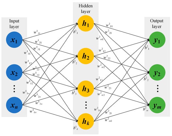
Figure 3.
Structure of the multilayer perceptron (MLP). The concept follows [29].
Forward propagation is a core step in MLP, in which neurons at each layer receive output from the previous layer and calculate the output of this layer through weighted summation and nonlinear activation functions. The input formula for the th neuron in the th layer is given in Formula (5):
where is the weight connecting the th neuron in th layer to the th neuron in the th layer; is the output of the th neuron in th layer; and is the bias of the th neuron in the th layer. A nonlinear activation function is applied to the input of the neuron, which is the output of the neuron. The output is given by Formula (6):
where the output will be used as the input of neurons in the next layer (th layer). In terms of activation function selection, the ReLU function is widely used in hidden layers because of its simple calculation process and high convergence speed. The MLP fitting model is constructed as follows:
- Input layer: The number of neurons (Nin) in the input layer is set according to the number of input characteristics.
- Hidden layer: The hidden layer uses an adaptive structural optimization mechanism, and the initial number of neurons (h0) and the number of structural optimizations (k) in the hidden layer are set to achieve evolutionary iteration of the hidden layer. Each round of iteration includes dynamic adjustment of neuron quantity, depth expansion of the hidden layer, and topological reconstruction of connections between hidden layers. The nonlinear activation function ReLU is uniformly used for each hidden layer.
- Output layer: The output layer structure is determined according to the task requirements. The number of neurons (Nout) in the output layer is set according to the number of output characteristics, and the maximum number of iterations (epochs) and learning rate (η) are set.
The MLP optimizes the weight and bias parameters in the network with the help of the back propagation algorithm [30]. When training the MLP network model, the training is carried out based on the back propagation algorithm. The input characteristic vector is used as training data, and the error between the calculated fitting result and the real label is back-propagated from the output layer to the input layer, thereby adjusting the network weights and bias parameters. Specifically, by solving the partial derivative of the error with respect to each weight and bias, the parameters are updated along the gradient descent direction to gradually reduce the error.
3.2. WOA-MLP Fitting Model
As the learning probability of the MLP fitting model is affected by engineering empirical factors, the WOA is introduced to optimize the learning probability of the MLP with the mean absolute error as the adaptive value to further improve the frequency characteristic fitting accuracy of the LLC under all operating conditions.
The WOA simulates the predatory behavior of whales, especially their distinctive spiral position-updating mechanism, enabling accelerated convergence toward the optimal solution. When the algorithm is close to the optimal solution, the exact location of the optimal solution can be found more accurately. In the WOA, the individual whales exhibit large-scale mobility within the search space through a hybrid approach combining stochastic search and directed search. The WOA features relatively few parameters, and the main parameters such as the population size and shrinkage factor have clear physical meanings and are relatively simple to adjust. Moreover, these parameters have a more intuitive impact on algorithm performance and are easy to set reasonably according to the characteristics of the problem.
The samples in the training set are fitted based on the MLP fitting model, and the current value of mean absolute error is updated after the current fitting. The learning probability of the MLP is iteratively optimized using the WOA and the current value of mean absolute error. The fitting model is updated based on the optimized learning probability before proceeding to the next fitting. This step is repeated until all training samples in the training set are fitted. Formula (7) is the formula for WOA optimized position update:
where is the solution vector of the whale position in the th iteration, i.e., the learning probability of the fitting model; is a random value in a linear spiral; is a computational vector per dimension; are parameter vectors calculated per dimension; is the distance between a whale and its prey. The WOA is employed to search for the hyperparameter vector of the MLP.
- Fitness (objective): validation loss, given by Formula (8):with magnitude MAE and unwrapped phase RMSE.
- Position encoding: each whale encodes (continuous dims normalized; discrete dims via index mapping).
- WOA updates given by Formula (9):
If , exploitation is performed around the best position otherwise, exploration is conducted around a randomly selected position .
- Decode/Train/Eval: decode , train the MLP with a fixed budget, and compute on the validation set as the fitness.
The steps for the random generation of whale positions are as follows:
- Normalize each hyperparameter to [0, 1] (discrete dims via index lists).
- Sample N initial whales
- Decode and repair: map , round discrete dims, and clip to feasible bounds if needed.
- Evaluate fitness to set the initial best .
Stopping criteria: The algorithm terminates once the iteration counter t reaches the maximum number of iterations (MaxIter). This condition indicates that the WOA has reached the maximum number of iterations.
The hyperparameters optimized by the WOA include both network architecture and training settings:
- Architecture: depth , width , ;
- Training: initial LR , weight decay , dropout , batch , early-stopping patience .
The rationale is as follows: Deployment constraints limit depth and width; risk of overfitting determines ; convergence and robustness inform . Unless phase noise dominates, the weighting coefficients are set as .
Figure 4 below is the optimization flow chart:
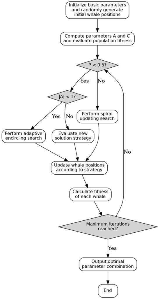
Figure 4.
Flow chart of the whale optimization algorithm.
3.3. FT-WOA-MLP Fitting Model
To overcome the problem of poor fitting accuracy of the WOA-MLP fitting model caused by changes in operating conditions and curve fluctuations, FT was introduced to fine-tune and optimize the WOA-MLP fitting model.
In order for the pre-trained model to be competent in identifying new datasets, the feature information extracted by the pre-trained model needs to be universal and fundamental. As WOA-MLP is a highly nonlinearly coupled fitting model, the information extracted by conventional neural networks is limited. The structure of the MLP can be divided into an underlying network and a top-level network. The features extracted from the underlying network are universal, so it is a network suitable for transfer learning.
Since the new fitting task in this paper is highly correlated with the pre-training task, the full model fine-tuning mode is adopted. The specific steps for fine-tuning the WOA-MLP model based on FT are as follows:
- Construction of pre-trained model: Similar to the construction of the WOA-MLP model, normalize the input feature quantity and then input it into the MLP training model. With MAE as the target value, use the WOA to perform spiral optimization iteration on the learning probability of MLP. Set the training cycle (epochs_pt) according to the amount of data and conduct training under all operating conditions.
- Construction of FT model: Remove the original fitting output layer in WOA-MLP, add a new specific task layer, introduce regularization constraints to enhance the generalization capabilities of the new layer, and freeze all pre-trained layer parameters to retain feature extraction capabilities.
- Hierarchical optimization training: Adjust the model structure, replace the top layer, and configure the learning rate (lr). Set the training cycle (epochs_ft) according to the amount of data and conduct training under all operating conditions. Select an appropriate optimizer and set the momentum coefficient (mom).
- FT training: Progressively fine-tune the model, freeze the feature extraction layer, train only the newly added task layer until convergence, and unfreeze the terminal pre-trained layer.
In the fine-tuning (FT) stage, the MLP is decomposed into a shared backbone and a task-specific head . During FT, the backbone parameters are frozen to preserve the general representation learned from the source dataset, while the task-specific head is re-initialized and trained with a small calibration set. In practice, the task-specific head is implemented as a lightweight linear (or dual linear) layer that separately outputs the magnitude and phase responses. The optimization objective remains the same as in the initial training but is now restricted to the small task layer, which substantially reduces the computational cost. Conceptually, the task-specific head captures domain or measurement shifts, such as scale differences, offsets, or mild shape variations, thereby enabling the model to adapt efficiently to a new converter or sub-domain without the need for re-running a full hyperparameter search.
4. Experimental Analysis
4.1. Experimental Conditions
Take an LLC SMPS module as an example, which has a rated input voltage of 530 V, a rated output voltage of 24 V, a rated output current of 54 A, an input voltage range of 380–710 V, and an output current of 6–72 A. Connect a 5 Ω excitation resistor in series in its voltage feedback circuit, and connect the two ends of the excitation resistor to the excitation signal generator and the oscilloscope, respectively; switch the oscilloscope probe to the AC position, and connect the signals at the injection end and the output end to the oscilloscope through the X1 probe to collect both the excitation signal and the response signal. The experimental setup for measuring the loop frequency response of the LLC prototype, including the injection point, oscilloscope, and signal generator, is shown in Figure 5.
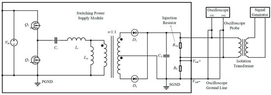
Figure 5.
Experimental connection diagram of the half-bridge LLC resonant converter with AC injection for frequency response measurement.
The experimental platform is shown in Figure 6 below.
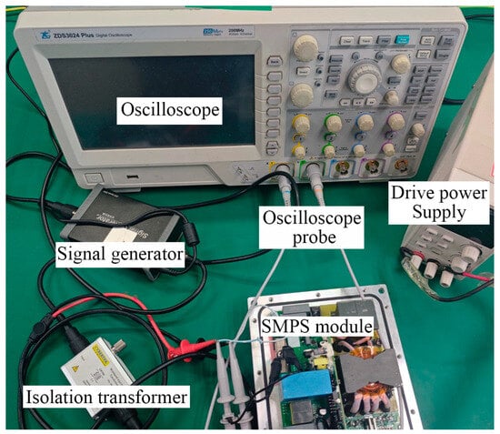
Figure 6.
Experimental platform.
The equivalent parameters of the tested prototype are summarized in Table 1.

Table 1.
Equivalent parameters of the tested LLC converter.
4.2. Frequency Characteristic Data Acquisition
4.2.1. Data Acquisition
The selected SMPS module has an input voltage range of 380–710 V and an output current range of 6–72 A. Within these ranges, a test matrix was designed using an equal-interval sampling method: for the input voltage, 12 discrete operating points uniformly selected in the range of 380–710 V at 30 V intervals; for the output current, 12 discrete operating points uniformly selected in the range of 6–72 A at 6 A intervals. The 12 input voltage values and the 12 output current values are orthogonally combined to form 144 (12 × 12) independent operating conditions covering the entire working area of the SMPS module.
For each preset operating condition, 81 frequency points were set in the frequency range of 10 Hz to 10 kHz for sweep frequency testing. Small signal disturbances were injected. The amplitude-frequency characteristics and phase-frequency characteristics of the module were recorded, and a frequency response curve was drawn. The result example is shown in Figure 7.
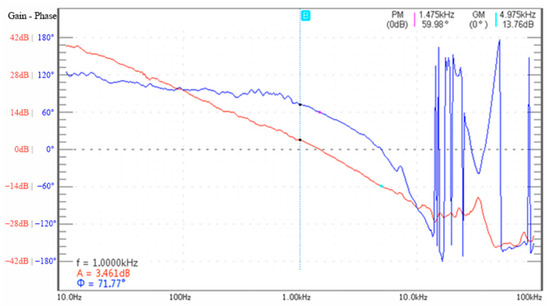
Figure 7.
Frequency characteristic curves.
In Figure 7, the red curve is the amplitude-frequency characteristic curve, and the blue curve is the phase-frequency characteristic curve. An orthogonal matrix of operating conditions and frequency points was utilized, collecting a total of 11,664 sets of frequency response characteristics data derived from 144 operating conditions and 81 frequency points.
The chosen sweep range of 10 Hz–10 kHz fully covers the control loop dynamics. The loop crossover frequency fc of the tested LLC converter is in the order of several hundred hertz. According to control design practice, scanning up to about one decade above the crossover frequency is sufficient to capture the loop gain and phase characteristics. Beyond this range, especially at frequencies close to the switching frequency (40–200 kHz), the loop gain has already dropped well below unity, and the response is dominated by switching harmonics and parasitic effects rather than by the feedback loop. Therefore, extending the sweep to higher frequencies would not provide additional information relevant to loop stability or performance, while it may introduce measurement noise. The selected frequency range thus adequately reflects the module’s performance.
4.2.2. Outlier Processing
Affected by the test environment, the collected amplitude-frequency and phase-frequency data contained some outliers. These outliers were processed using the mean shift method, replacing the outlier with the mean calculated from its 10 preceding and 10 subsequent groups.
4.2.3. Dataset Division
A grouped cross-distribution strategy was employed for dataset division: A total of 144 operating conditions were sequentially divided into 48 groups (three per group). Within each group, the first two operating conditions were assigned to the training set, while the third operating condition was assigned to the test set. Finally, the training set contained 96 operating conditions, and the test set contained 48.
For clarity and reproducibility, the training process is accompanied by a detailed summary of the dataset employed in this work together with the information provided to the MLP. Table 2 presents the dataset summary, including the number of operating points, sweep frequencies, ranges, and total samples. Table 3 further details the inputs, targets, and preprocessing steps employed for MLP training. All simulations and analyses in this work were carried out using MATLAB R2023a (including its toolboxes for data processing, curve fitting, and model training).

Table 2.
Dataset summary used to train the MLP.

Table 3.
Information used for MLP training.
4.3. Model Parameter Setting
4.3.1. MLP Parameter Setting
The parameters of the MLP fitting model were set as follows:
- Input layer: The number of neurons is determined by the number of input features. The input feature quantities include input voltage U, output current I, and injection frequency F. Let the number of neurons in the input layer Nin = 3.
- Hidden layer: Dynamically optimize the neurons in the hidden layer according to training errors and computing resources, and adaptively adjust the number of neurons or number of hidden layers. Assume that the initial number of neurons in the hidden layer h0 = 10 and the number of structural optimizations k = 5.
- Output layer: Determine the number of neurons and activation function according to the fitting target. The number of neurons is equal to the number of output features. The output feature quantity includes amplitude-frequency and phase-frequency. Let the number of neurons in the output layer Nout = 2; let the maximum number of training epochs = 500, and the learning rate η = 0.01; use ReLU as the activation function.
The parameters are shown in Table 4:

Table 4.
Parameter settings of the MLP model.
4.3.2. Horizontal Comparison Between MLP and WNN
In order to verify the advantages of the MLP compared with other mainstream fitting algorithms, a wavelet neural network (WNN) model was selected for comparative analysis [31]. The WNN is a type of neural network that combines wavelet analysis theory with an artificial neural network, uses wavelet function as the transfer function of hidden layer nodes, and propagates signals forward while errors propagate backward.
The MLP and WNN were employed to perform amplitude-frequency and phase-frequency fitting across input voltages of 380–710 V, output currents of 6–72 A, and switching frequencies in the range of 10 Hz–10 kHz, with subsequent comparison of fitting errors. Table 5 shows the comparison of amplitude-frequency fitting errors, where each error value was calculated across all operating conditions in the test set.

Table 5.
Comparison of amplitude-frequency fitting errors between MLP and WNN.
The amplitude-frequency fitting accuracy of the MLP model was higher than that of the WNN model, with MAE reduced by 8.71%, MAPE reduced by 42.5%, RMSE reduced by 21.63%, and R2 increased by 13.04%. Table 6 shows the comparison of phase-frequency fitting errors, where each error value was calculated across all operating conditions in the test set.

Table 6.
Comparison of phase-frequency fitting errors between MLP and WNN.
The phase-frequency fitting accuracy of the MLP model was also higher than that of the WNN model, with MAE reduced by 35.38%, MAPE reduced by 41.02%, RMSE reduced by 30.07%, and R2 increased by 13.64%. Based on the horizontal comparison above, the MLP demonstrated a pronounced advantage over the WNN across four error metrics.
4.3.3. WOA Parameter Setting
WOA parameters were set as follows:
- Optimization objectives: Given that the amplitude-frequency and phase-frequency characteristics were fitted separately to establish a dual-objective optimization framework, set the output variable dimension dim = 1; select the MAE as the fitness function to ensure the fitting accuracy.
- Population and iteration configuration: To balance exploration and development capabilities, set population size = 20; to ensure full convergence of large datasets (>10 k samples), set the maximum number of iterations epochs = 400.
- Setting of dual iteration mechanism: The outer layer iteration completes the WOA global optimization process; the inner layer iteration fine-tunes the learning probability in MLP, with the number of FT iterations set as opt = 30.
The parameters are shown in Table 7:

Table 7.
WOA parameter setting.
4.3.4. Model FT Parameter Setting
The FT parameters were set as follows:
- Learning rate configuration: Use the hierarchical learning rate mechanism, with the learning rate of top task layer set as lr_top ∈ [10−2, 10−4] and the learning rate of bottom feature extraction layer set as lr_bottom ∈ [10−2, 10−6]. Learning rate optimization was achieved through the Bayesian hyperparameter optimization framework [32].
- Optimizer configuration: Use the stochastic gradient descent (SGD) algorithm and introduce momentum coefficient, with the momentum coefficient at the initial stage set as mom_init = 0.8 and the momentum coefficient at the convergence stage set as mom_final = 0.95.
- Training cycle setting: To ensure full convergence of large datasets (>10 k samples), set the number of pre-trained model iterations epochs_pt = 400; to prevent overfitting, set the number of FT iterations epochs_ft = 200.
- Structural configuration: Unfreeze the last two pre-trained layers in the fine-tuning stage for end-to-end optimization.
The parameters are shown in Table 8:

Table 8.
FT parameter setting.
4.4. Comparison of Amplitude-Frequency Characteristics
The MLP, WOA-MLP, and FT-WOA-MLP were used to fit the amplitude-frequency characteristics within the full operating range of input voltage 380–710 V, output current 6–72 A, and injection frequency 10 Hz–10 kHz. After the fitting model was trained, the test set covering all operating conditions was input into the model to calculate the fitting error, followed by a comparative analysis. Table 9 shows the comparison results, where each error value was calculated across all operating conditions in the test set.

Table 9.
Comparison of amplitude-frequency fitting errors in the MLP family.
Figure 8 systematically compares the performance of three models (MLP, WOA-MLP, and FT-WOA-MLP) during amplitude-frequency fitting training in terms of four error metrics. The four subplots, respectively, show the dynamic change trends of MAE, MAPE, RMSE, and R2 metrics with respect to the training epochs:
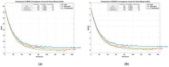
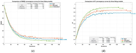
Figure 8.
Iterative comparison of different errors for multiple models during amplitude-frequency fitting. (a) MAE; (b) MAPE; (c) RMSE; (d) R2.
By analyzing the data in Table 9 and Figure 8, it can be seen that compared with the WOA-MLP fitting model, the FT-WOA-MLP fitting model demonstrated a higher fitting accuracy: a 35% reduction in MAE, a 61% reduction in MAPE, a 51% reduction in RMSE, and a 7% increase in R2. Compared with the MLP model, it also showed a higher fitting accuracy: a 53% reduction in MAE, an 83% reduction in MAPE, a 37% reduction in RMSE, and an 18% increase in R2. The total number of iterations were 160, 148, and 125 for the MLP, WOA-MLP, and FT-WOA-MLP models, respectively. The FT-WOA-MLP model entered the convergence stage earlier than WOA-MLP and MLP models in the iteration process and could complete the amplitude-frequency fitting task faster.
An input voltage of 530 V was selected to observe the amplitude-frequency changes with current and frequency, as shown in Figure 9. An output current of 54 A was selected to observe the amplitude-frequency changes with voltage and frequency, as shown in Figure 10.
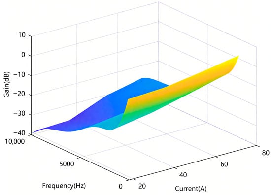
Figure 9.
Three-dimensional diagram of amplitude-frequency changes with current and frequency.
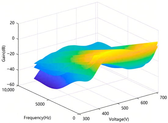
Figure 10.
Three-dimensional diagram of amplitude-frequency changes with voltage and frequency.
In Figure 9 and Figure 10, the colors represent the gain (in dB), with the color gradient transitioning from blue to yellow. Blue indicates lower gain values (more negative dB), while yellow represents higher gain values (more positive dB). The intensity of the color corresponds to the magnitude of the gain, with blue representing lower gain and yellow indicating higher gain. This color gradient visually represents the variation in gain across different current/voltage and frequency conditions.
Figure 11 presents fitted-versus-measured amplitude-frequency curves under three representative operating conditions: 380 V/18 A (minimum), 530 V/54 A (rated), and 710 V/72 A (maximum). Each subplot contains four curves: Measured, MLP, WOA-MLP, and FT-WOA-MLP. To avoid redundancy, the complete set of amplitude-frequency comparisons—covering input voltages 380/530/710 V and output currents 18/36/54/72 A, including the cases of different currents at fixed voltages—is provided in the Supplementary Materials with identical axes, legends, and metrics.

Figure 11.
Amplitude-frequency comparisons at three operating points. (a) 380 V/18 A; (b) 530 V/54 A; (c) 710 V/72 A.
According to the above figure, it is evident that the FT-WOA-MLP model exhibited a better fitting performance, with its amplitude-frequency curve aligning more closely with the actual curve compared with the WOA-MLP model. The model achieved precise fitting for both low-voltage operating conditions and the end of amplitude-frequency curves, enabling accurate fitting of amplitude-frequency characteristics under all operating conditions.
4.5. Comparison of Phase-Frequency Characteristics
The MLP, WOA-MLP and FT-WOA-MLP models were used to fit the phase-frequency characteristics within the full operating range of input voltage 380–710 V, output current 6–72 A, and injection frequency 10 Hz–10 kHz. After the fitting model was trained, the test set covering all operating conditions was input into the model to calculate the fitting error, followed by a comparative analysis. Table 10 shows the comparison results, where each error value was calculated across all operating conditions in the test set.

Table 10.
Comparison of phase-frequency fitting errors in the MLP family.
Figure 12 systematically compares the performance of three models (MLP, WOA-MLP, and FT-WOA-MLP) during phase-frequency fitting training in terms of four error metrics. The four subplots respectively show the dynamic change trends of MAE, MAPE, RMSE, and R2 metrics with respect to the training epochs:
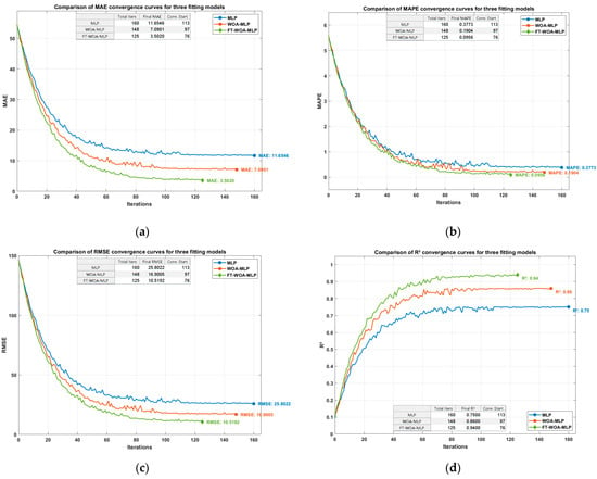
Figure 12.
Iterative comparison of different errors for multiple models during phase-frequency fitting. (a) MAE; (b) MAPE; (c) RMSE; (d) R2.
By analyzing the data in Table 10 and Figure 12, it can be seen that compared with the WOA-MLP fitting model, the FT-WOA-MLP fitting model demonstrated a higher fitting accuracy: a 52% reduction in MAE, a 49% reduction in MAPE, a 38% reduction in RMSE, and a 9% increase in R2. Compared with the MLP model, it also showed a higher fitting accuracy: a 70% reduction in MAE, a 75% reduction in MAPE, a 60% reduction in RMSE, and a 25% increase in R2. The total number of iterations were 160, 148, and 125 for MLP, WOA-MLP, and FT-WOA-MLP models, respectively. The FT-WOA-MLP model entered the convergence stage earlier than the WOA-MLP and MLP models in the iteration process and could complete the phase-frequency fitting task faster.
An input voltage of 530 V was selected to observe the phase-frequency changes with current and frequency, as shown in Figure 13. An output current of 54 A was selected to observe the phase-frequency changes with voltage and frequency, as shown in Figure 14.
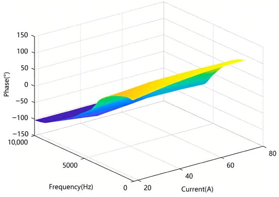
Figure 13.
Three-dimensional diagram of phase-frequency changes with current and frequency.
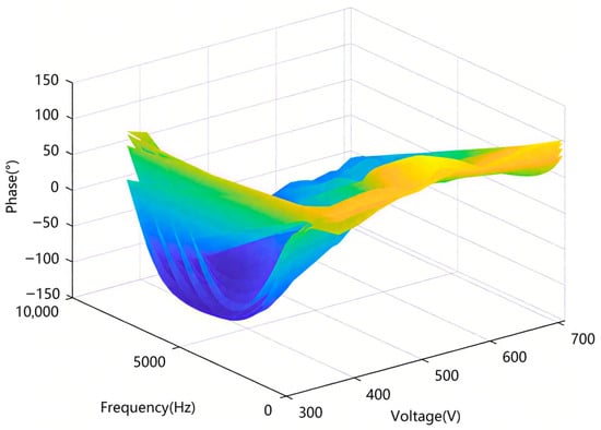
Figure 14.
Three-dimensional diagram of phase-frequency changes with voltage and frequency.
In Figure 13 and Figure 14, the colors represent the phase angle (in degrees), with the color gradient ranging from blue to yellow. Blue indicates negative phase values, while yellow represents positive phase values. The intensity of the color corresponds to the magnitude of the phase shift, with blue indicating lower phase values and yellow indicating higher phase values. The color gradient effectively visualizes the phase changes across varying current/voltage and frequency values.
Figure 15 presents fitted-versus-measured phase-frequency curves under three representative operating conditions, namely 380 V/18 A (minimum), 530 V/54 A (rated), and 710 V/72 A (maximum). Each subplot contains four curves: measured, MLP, WOA-MLP, and FT-WOA-MLP. To avoid redundancy, the complete set of phase-frequency comparisons—covering input voltages 380/530/710 V and output currents 18/36/54/72 A, including the cases of different currents at fixed voltages—is provided in the Supplementary Materials with identical axes, legends, and metrics.

Figure 15.
Phase-frequency comparisons at three operating points. (a) 380 V/18 A; (b) 530 V/54 A; (c) 710 V/72 A.
The graphical comparisons above reveal distinct phase-frequency fitting performance across varying operating conditions, and the phase-frequency characteristic curve under continuous operating conditions was obtained. Compared with the WOA-MLP model, the FT-WOA-MLP model exhibited higher fitting accuracy and closer alignment with the actual phase-frequency characteristics. It can effectively respond to changes in different operating conditions and address the problem of excessive fitting error at low-input-voltage operating points.
4.6. Comparison with Analytical Models
Figure 16 shows the comparison at the 530 V/54 A operating condition. As can be observed, the FHA model exhibits sizable deviations in the decade around the crossover frequency , mainly because it neglects the output pole and the transport delay, and it produces an unrealistic high-frequency trend. In contrast, the improved averaged model correctly reproduces the −20 dB/dec slope near , the kHz-range ESR shoulder, and the additional high-frequency phase lag, making it the most informative and interpretable analytical baseline.
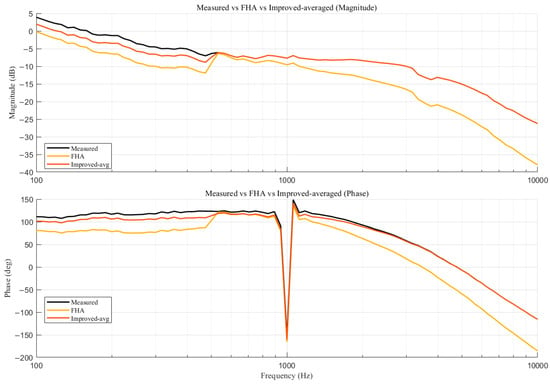
Figure 16.
Comparison of measured frequency response with FHA and improved-averaged models at 530 V/54 A operating condition: magnitude characteristics (top) and phase characteristics (bottom). The FHA derivation is provided in Appendix A.
Figure 16 juxtaposes the measured loop with two analytical models: the plain FHA and an improved averaged model that augments FHA by the output-side dynamics and a compact delay.
- Magnitude (top): Around the bandwidth (), the measurement rolls off at −20 dB/dec. The improved averaged curve almost coincides with the measurement, whereas FHA remains too flat and underestimates the slope. At a few kHz, the measurement shows a mild shoulder caused by the ESR zero; the improved model reproduces this feature through , while FHA misses it and diverges at higher frequencies.
- Phase (bottom): Near the bandwidth, the improved model follows the measured bend; at higher frequencies, it also captures the additional lag caused by sampled-data/transport delay (). FHA lacks both mechanisms, hence the wrong bend location and decay trend.
Classical averaging (incl. FHA) systematically fails in the 102–103 Hz decade because it ignores the output pole/ESR zero and the effective delay of the modulation/measurement chain. An improved averaged model that keeps FHA’s interpretability but explicitly includes these two elements correctly reproduces the −20 dB/dec slope near fc, the ESR-induced shoulder, and the high-frequency phase lag, while remaining lightweight.
4.7. Practical Application Case Study: Defect Identification and Quality Control
To further demonstrate the practical utility of the proposed FT-WOA-MLP model, a case study is presented on how the method can be applied in production-line quality control for LLC resonant SMPS units.
The goal is to identify potential defects during mass production by comparing the measured loop frequency response of each unit with the model-predicted “digital golden standard”, thereby ensuring product consistency and reliability.
Application Scenario: A newly assembled SMPS unit is placed on the experimental test platform. A challenging operating condition—low input voltage of 380 V and high output current of 72 A—is selected for testing, as loop instabilities or component tolerance issues are most likely to appear under such conditions.
Step 1—Model Prediction. The parameters (380 V, 72 A) are fed into the trained FT-WOA-MLP model, which instantly generates the expected amplitude- and phase-frequency curves for a healthy unit. These curves act as the digital golden standard.
Step 2—Measurement. A spot frequency sweep is performed on the physical unit at the same condition, yielding its actual frequency response. Compared with full characterization, this requires only a single operational point and thus is highly efficient.
Step 3—Comparison and Diagnosis.
- Scenario A (healthy unit): If the measured response closely matches the predicted curves (similar to the agreement shown in Figure 10), the unit passes the quality check.
- Scenario B (defective unit): If a significant deviation is detected—for example, a measured phase margin reduced by 15° or the appearance of an unexpected resonance peak—the system flags the unit as defective. Such deviations may stem from a wrong capacitor value, a faulty solder joint, or incorrect transformer inductance. The unit can then be sent for detailed inspection and rework.
This approach (i) improves efficiency by replacing multi-condition sweeps with quick spot checks, (ii) provides objectivity through quantitative comparison, (iii) offers comprehensive coverage since the model is trained across all operating conditions, and (iv) supports automation, enabling 100% testing on production lines.
4.8. Closed-Loop Characteristics
To further verify the closed-loop behavior of the LLC converter, frequency-domain characteristics were measured and are presented in Figure 17, Figure 18 and Figure 19.
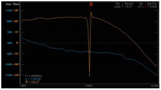
Figure 17.
Measured loop Bode at .
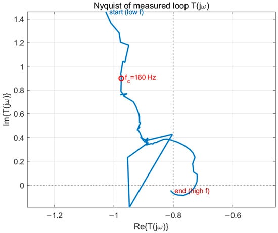
Figure 18.
Nyquist plot of the measured loop .
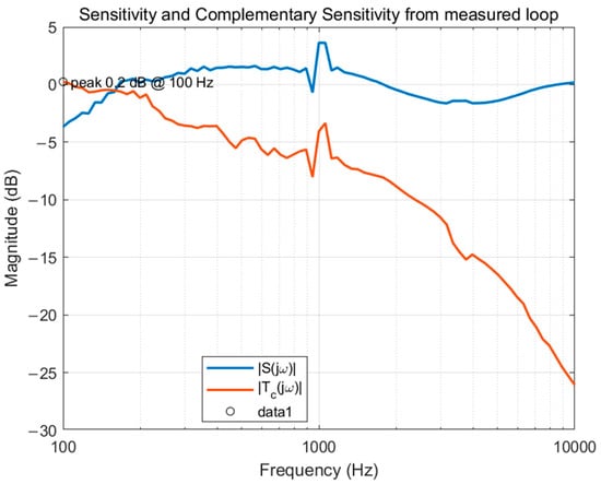
Figure 19.
Measured and . The small peak and rapid high-frequency roll-off indicate benign resonances and good noise-shaping.
Figure 17 shows the measured Bode diagram of the control loop at the nominal operating point (). The crossover frequency is approximately , with a phase margin of and a gain margin of , confirming a stable and well-compensated loop. Figure 18 reports the Nyquist locus of the measured loop gain ; the trajectory does not encircle the point , thereby verifying robust stability in accordance with the Nyquist criterion. Figure 19 depicts the sensitivity function and complementary sensitivity function . The curve exhibits only a small peak (≈0.2 dB) and decays rapidly above , indicating effective high-frequency noise rejection and benign resonances. The low-frequency behavior of is consistent with the deliberately selected low crossover, highlighting robustness-oriented compensation. Collectively, these results demonstrate that the proposed control loop achieves both robust stability and favorable disturbance/noise shaping.
5. Conclusions
This work proposes an FT-WOA-MLP-based fitting method for accurately modeling the frequency characteristics of LLC SMPS under all operating conditions. Experimental validation demonstrates that the model achieves high accuracy: for amplitude-frequency fitting, the FT-WOA-MLP reduced MAE, MAPE, and RMSE by 35%, 61%, and 51%, respectively, with R2 improved by 7% over WOA-MLP; for phase-frequency fitting, MAE, MAPE, and RMSE were reduced by 52%, 49%, and 38%, with R2 increased by 9%. These results confirm the method’s ability to provide reliable full-domain frequency–response prediction.
The proposed approach offers several advantages: (i) accurate fitting across the full operating range; (ii) robustness to measurement noise and outliers; (iii) improved convergence through WOA-assisted tuning; (iv) enhanced adaptability to related prototypes via FT; and (v) suitability as a lightweight surrogate in design and analysis tools. Limitations include the need for seed experimental data, unreliable extrapolation beyond the trained range, the requirement of model retuning after major hardware changes, and the lack of direct physical interpretability without analytical support.
The study focuses on the MLP family (MLP, WOA-MLP, and FT-WOA-MLP) rather than heavier architectures for reasons of fairness and deployability: MLP models meet embedded resource constraints, train stably on modest laboratory datasets, and allow clear attribution of incremental improvements due to optimization strategies. Overall, the proposed method provides a practical surrogate for closed-loop frequency characteristics, supporting loop-stability analysis and defect identification across the full operating domain of LLC SMPS.
Supplementary Materials
The following supporting information can be downloaded at: https://www.mdpi.com/article/10.3390/jlpea15040057/s1, Figure S1: Comparison of fitted amplitude-frequency curves across multiple models under varying currents at a low voltage of 380 V; Figure S2: Comparison of fitted amplitude-frequency curves across multiple models under varying currents at a rated voltage of 530 V; Figure S3: Comparison of fitted amplitude-frequency curves across multiple models under varying currents at a high voltage of 710 V; Figure S4: Comparison of fitted phase-frequency curves across multiple models under varying currents at a low voltage of 380 V; Figure S5: Comparison of fitted phase-frequency curves across multiple models under varying currents at a rated voltage of 530 V; Figure S6: Comparison of fitted phase-frequency curves across multiple models under varying currents at a high voltage of 710 V.
Author Contributions
Conceptualization, J.G. and R.H.; methodology, J.G.; software, R.H.; validation, J.G., R.H. and Z.Y.; formal analysis, R.L.; investigation, R.L.; resources, L.Z.; data curation, J.G.; writing—original draft preparation, J.G.; writing—review and editing, G.A.; visualization, Z.Y.; supervision, G.A.; project administration, L.Z.; funding acquisition, G.A. All authors have read and agreed to the published version of the manuscript.
Funding
This research was funded by the Shijiazhuang Industry-University-Research Collaboration Project for Higher Education Institutions in Hebei Province, “Research on Key Technologies for Dynamic Performance Analysis and Transfer Function Identification of DC Power Conversion Modules” (No. 241060171A).
Data Availability Statement
The original contributions presented in this study are documented within the article. For additional information, please contact the corresponding author.
Conflicts of Interest
Authors R.L. and L.Z. were employed by the company Shijiazhuang Tonhe Electronics Technologies Co., Ltd. All other authors state that they have no competing financial or personal relationships that could have influenced the work presented in this article.
Appendix A
Analytical Small-Signal Derivation of an LLC Resonant Converter (FHA)
- Assumptions and notation (FHA framework)
- Half-bridge excitation with 50% duty; switches and rectifier are ideal.
- Only fundamental (first harmonic) components of voltages/currents are retained.
- The output capacitor Co is large so that the DC ripple is small; the load is Ro.
- Secondary rectifier and load are referred to the primary by an AC resistance chosen to preserve power.
Primary-referred AC load (full-wave rectification, half-bridge) is given by Formula (A1):
where n is the primary-to-secondary turns ratio.
- 2.
- Fundamental source and tank model
The half-bridge square wave is replaced by its fundamental sinusoid of amplitude, given by Formula (A2):
With resonant elements Lr and Cr in series and magnetizing inductance Lm in parallel with , the series and parallel impedances and the tank transfer are given in Formula (A3):
- 3.
- AC–DC linkage (power consistency)
The primary AC power absorbed by equals the DC output power (lossless FHA), given by Formula (A4):
In steady state, this yields the familiar DC gain scaling (often absorbed into constants in small-signal work), given by Formula (A5):
- 4.
- Small-signal control-to-output path under frequency modulation (PFM)
In LLC control, the command perturbs the switching (excitation) angular frequency through an FM/VCO path, given by Formula (A6):
The output is linearized around the operating point , and the chain rule is applied, given by Formula (A7):
so the FHA small-signal control-to-output transfer is given in Formula (A8):
- 5.
- Loop formation and sensitivity functions
With a compensator (e.g., Type-II/III), the open loop is given in Formula (A9):
and the usual sensitivity/complementary sensitivity are given in Formula (A10):
References
- Kanale, A.; Agarwal, A.; Baliga, B.J.; Bhattacharya, S. Monolithic Reverse Blocking 1.2 kV 4H-SiC Power Transistor: A Novel, Single-Chip, Three-Terminal Device for Current Source Inverter Applications. IEEE Trans. Power Electron. 2022, 37, 10112–10116. [Google Scholar] [CrossRef]
- Kamarajugadda, N.; Fernandes, B.G.; Chatterjee, K. GaN-Based High Power Density Multifunctional Onboard Charger for Electric Vehicles Eliminating Auxiliary Power Module. IEEE Trans. Ind. Electron. 2025, 72, 7920–7931. [Google Scholar] [CrossRef]
- Hertel, J.C.; Overgaard, J.E.F.; Jorgensen, I.H.H.; Andersen, T.M.; Rodgaard, M.; Knott, A. Synchronous Rectifier for High-Frequency Switch-Mode Power Supplies Using Phase-Locked Loops. IEEE J. Emerg. Sel. Top. Power Electron. 2020, 8, 2227–2237. [Google Scholar] [CrossRef]
- Kurimoto, Y. A High Precision Power Supply for Fast Pulse Current with a Digital Control System. IEEE Trans. Appl. Supercond. 2016, 26, 1–4. [Google Scholar] [CrossRef]
- Funaki, H.; Noge, Y.; Shoyama, M.; Yonezawa, Y.; Miyazawa, A. Construction of HILS System for LLC Resonant Converter Using LPV Model. IEEE Trans. Ind. Appl. 2024, 60, 3297–3305. [Google Scholar] [CrossRef]
- Xu, Y.; You, W.; Zhang, Z.; Wu, H.; Jin, T. Hybrid Energy System for Urban Rail Power Supply Based on Multi-Level Multi-Port LCC Resonant Converters. IEEE Trans. Transp. Electrif. 2025, 11, 8987–8999. [Google Scholar] [CrossRef]
- Park, W.; Namgoong, G.; Choi, E.; Bien, F. An On-/Off-Time Sensing-Based Load-Adaptive Mode Control of Triple Mode Buck Converter for Implantable Medical Devices. IEEE Trans. Biomed. Circuits Syst. 2023, 17, 585–597. [Google Scholar] [CrossRef]
- Gao, Y.; Kang, B.; Chen, Y.; Zhao, Y.; Zhang, W.; Fan, Y. A Simple and All-Optical Microwave Doppler Frequency Shift and Phase Measurement System Based on Sagnac Loop and I/Q Detection. IEEE Trans. Instrum. Meas. 2021, 70, 1–9. [Google Scholar] [CrossRef]
- Yang, J.; Yan, T.; Sun, W. Polynomial Fitting and Interpolation Method in TDOA Estimation of Sensors Network. IEEE Sens. J. 2023, 23, 3837–3847. [Google Scholar] [CrossRef]
- Yutthagowith, P.; Baba, Y. An Effective Approximate Mathematical Expression for Non-Linear Resistance Characteristics of Metal Oxide Elements. IEEE Trans. Electromagn. Compat. 2025, 67, 988–995. [Google Scholar] [CrossRef]
- Ramos-Frutos, J.; Miguel-Andrés, I.; Oliva, D.; Pérez-Cisneros, M.; Alonso-Rasgado, T.; Bailey, C.G.; Francisco Del Valle-Mojica, J. Digital Image Processing Applied in the Deformation Analysis of Hip Prosthesis: Multivariate Regression Analysis. IEEE Access 2024, 12, 176938–176948. [Google Scholar] [CrossRef]
- Long, C.; Hu, Q.; Zhao, M.; Li, D.; Ouyang, Z.; Yan, D.-M. A Triple-Stage Robust Ellipse Fitting Algorithm Based on Outlier Removal. IEEE Trans. Instrum. Meas. 2023, 72, 1–14. [Google Scholar] [CrossRef]
- Wenting, M.; Mingyao, M. Shading Fault Detection Method for Household Photovoltaic Power Stations Based on Inherent Characteristics of Monthly String Current Data Mapping. CSEE J. Power Energy Syst. 2023, 9, 1370–1382. [Google Scholar]
- Ren, L.; Dong, J.; Wang, X.; Meng, Z.; Zhao, L.; Deen, M.J. A Data-Driven Auto-CNN-LSTM Prediction Model for Lithium-Ion Battery Remaining Useful Life. IEEE Trans. Ind. Inform. 2021, 17, 3478–3487. [Google Scholar] [CrossRef]
- Ibude, F.; Otebolaku, A.; Ameh, J.E.; Ikpehai, A. Multi-Timescale Energy Consumption Management in Smart Buildings Using Hybrid Deep Artificial Neural Networks. J. Low Power Electron. Appl. 2024, 14, 54. [Google Scholar] [CrossRef]
- Gan, Z.; He, D.; Wu, P.; Xiong, B.; Zeng, N.; Zou, F.; Guo, F.; Bao, Q.; Zhao, F. CCD Standard Curve Fitting for Microarray Detection Base on Multi-Layer Perceptron. IEEE Photon. J. 2024, 16, 1–11. [Google Scholar] [CrossRef]
- Li, W.; Wang, X.; Wang, L.; Jia, L.; Song, R.; Fu, Z.; Xu, W. An LSTM and ANN Fusion Dynamic Model of a Proton Exchange Membrane Fuel Cell. IEEE Trans. Ind. Inform. 2023, 19, 5743–5751. [Google Scholar] [CrossRef]
- Aguirre, F.L.; Gomez, N.M.; Pazos, S.M.; Palumbo, F.; Suñé, J.; Miranda, E. Minimization of the Line Resistance Impact on Memdiode-Based Simulations of Multilayer Perceptron Arrays Applied to Pattern Recognition. J. Low Power Electron. Appl. 2021, 11, 9. [Google Scholar] [CrossRef]
- Zhang, Y.; Li, S.; Yi, W.; Yang, Y.; Cao, K.; Luo, B. A Robust Model Predictive Current Closed-Loop Control with Parameter Estimation Strategy Based on Immune Chaotic Antipredator PSO for PMSM. IEEE Trans. Power Electron. 2025, 40, 1836–1848. [Google Scholar] [CrossRef]
- Memon, M.A.; Siddique, M.D.; Mekhilef, S.; Mubin, M. Asynchronous Particle Swarm Optimization-Genetic Algorithm (APSO-GA) Based Selective Harmonic Elimination in a Cascaded H-Bridge Multilevel Inverter. IEEE Trans. Ind. Electron. 2022, 69, 1477–1487. [Google Scholar] [CrossRef]
- Khurshaid, T.; Wadood, A.; Gholami Farkoush, S.; Yu, J.; Kim, C.-H.; Rhee, S.-B. An Improved Optimal Solution for the Directional Overcurrent Relays Coordination Using Hybridized Whale Optimization Algorithm in Complex Power Systems. IEEE Access 2019, 7, 90418–90435. [Google Scholar] [CrossRef]
- Ahmad, N.S. Modeling and Hybrid PSO-WOA-Based Intelligent PID and State-Feedback Control for Ball and Beam Systems. IEEE Access 2023, 11, 137866–137880. [Google Scholar] [CrossRef]
- Krishnamoorthy, S.K.; Das, N.; Gudimetla, P.; Emami, K. Enhanced Speed Control for BLDC Motors Using WOA-Integrated PID Controller Optimization. IEEE Access 2024, 12, 162465–162475. [Google Scholar] [CrossRef]
- Yabalar, M.H.; Ercelebi, E. Hybrid Optimization Based Harmonic Minimization in Three Phase Multilevel Inverter with Reduced Switch Topology. IEEE Access 2024, 12, 71010–71023. [Google Scholar] [CrossRef]
- Vrbancic, G.; Podgorelec, V. Transfer Learning with Adaptive Fine-Tuning. IEEE Access 2020, 8, 196197–196211. [Google Scholar] [CrossRef]
- Lv, H.; Zhang, L.; Wang, Y. Improving DNN Accuracy on MLC PIM via Non-Ideal PIM Device Fine-Tuning. IEEE Trans. Comput.-Aided Des. Integr. Circuits Syst. 2025, 44, 2277–2286. [Google Scholar] [CrossRef]
- Zhou, Y.; Zhang, Q.; Huang, T.; Cai, Z. Prior Knowledge-Augmented Meta-Learning for Fine-Grained Fault Diagnosis. IEEE Trans. Ind. Inform. 2024, 20, 8115–8124. [Google Scholar] [CrossRef]
- Liang, J.; Liang, Q.; Wu, Z.; Chen, H.; Zhang, S.; Jiang, F. A Novel Unsupervised Deep Transfer Learning Method with Isolation Forest for Machine Fault Diagnosis. IEEE Trans. Ind. Inform. 2024, 20, 235–246. [Google Scholar] [CrossRef]
- Jabin, M.A.; Fok, M.P. Prediction of 12 Photonic Crystal Fiber Optical Properties Using MLP in Deep Learning. IEEE Pho-Tonics Technol. Lett. 2022, 34, 391–394. [Google Scholar]
- Qin, H.; Peng, J.; Xie, S.; Mo, Y.; Xiu, Q.; Chen, W. Switching Characteristics Analysis and Power Loss Minimization of SiC BJT Based on Dual Power Supply RC Driving Circuit. Energy Rep. 2022, 8, 710–720. [Google Scholar] [CrossRef]
- Jiang, F.; Dong, L.; Dai, Q. Designing a Mixed Multilayer Wavelet Neural Network for Solving ERI Inversion Problem with Massive Amounts of Data: A Hybrid STGWO-GD Learning Approach. IEEE Trans. Cybern. 2022, 52, 925–936. [Google Scholar] [CrossRef] [PubMed]
- Sukhorukov, M.P.; Kremzukov, Y.A.; Yudintsev, A.G.; Rulevskiy, V.M. Solar-Hydrogen System of Additional Power Supply and Digital Control System for on-Board Power Supply System. Int. J. Hydrogen Energy 2024, 88, 344–357. [Google Scholar] [CrossRef]
Disclaimer/Publisher’s Note: The statements, opinions and data contained in all publications are solely those of the individual author(s) and contributor(s) and not of MDPI and/or the editor(s). MDPI and/or the editor(s) disclaim responsibility for any injury to people or property resulting from any ideas, methods, instructions or products referred to in the content. |
© 2025 by the authors. Licensee MDPI, Basel, Switzerland. This article is an open access article distributed under the terms and conditions of the Creative Commons Attribution (CC BY) license (https://creativecommons.org/licenses/by/4.0/).