Abstract
Biologging refers to the use of animal-borne recording devices to study wildlife behavior. In the case of audio recording, such devices generate large amounts of data over several months, and thus require some level of processing automation for the raw data collected. Academics have widely adopted offline deep-learning-classification algorithms to extract meaningful information from large datasets, mainly using time-frequency signal representations such as spectrograms. Because of the high deployment costs of animal-borne devices, the autonomy/weight ratio remains by far the fundamental concern. Basically, power consumption is addressed using onboard mass storage (no wireless transmission), yet the energy cost associated with data storage activity is far from negligible. In this paper, we evaluate various strategies to reduce the amount of stored data, making the fair assumption that audio will be categorized using a deep-learning classifier at some point of the process. This assumption opens up several scenarios, from straightforward raw audio storage paired with further offline classification on one side, to a fully embedded AI engine on the other side, with embedded audio compression or feature extraction in between. This paper investigates three approaches focusing on data-dimension reduction: (i) traditional inline audio compression, namely ADPCM and MP3, (ii) full deep-learning classification at the edge, and (iii) embedded pre-processing that only computes and stores spectrograms for later offline classification. We characterized each approach in terms of total (sensor + CPU + mass-storage) edge power consumption (i.e., recorder autonomy) and classification accuracy. Our results demonstrate that ADPCM encoding brings 17.6% energy savings compared to the baseline system (i.e., uncompressed raw audio samples). Using such compressed data, a state-of-the-art spectrogram-based classification model still achieves 91.25% accuracy on open speech datasets. Performing inline data-preparation can significantly reduce the amount of stored data allowing for a 19.8% energy saving compared to the baseline system, while still achieving 89% accuracy during classification. These results show that while massive data reduction can be achieved through the use of inline computation of spectrograms, it translates to little benefit on device autonomy when compared to ADPCM encoding, with the added downside of losing original audio information.
1. Introduction
Biologging is the study of animal behavior through the use of electronic devices. Inferring behaviors requires a large amount of data, which have been made possible through increasingly energy-efficient recording embedded systems. However, manually processing the generated datasets becomes progressively more time-consuming, if not impossible. In this study, we focus on data recording and analysis. While commercial devices for embedded geolocation or movement analysis are common and readily available, this is not the case for animal-borne audio recorders. Scientists either adapt Passive Acoustic Monitoring (PAM) devices [1] or rely on academic attempts to develop custom designs [2,3]. In this context, over the past few years, we designed our own solution for embedded audio recording. Our device engineering is strongly driven by weight over autonomy ratio and exhibits cutting-edge power efficiency, being able to collect about 900 h of 16-bit 8 kHz audio data (~50 GB uncompressed audio samples) from a single small 1800 mAh Li-Ion battery [4]. In this application, recorded data are not streamed over an RF link, but rather stored onto an SD memory card for obvious energy-saving reasons. Still, our measurements demonstrate that data storage activity significantly contributes to the total power consumption when no audio data reduction is applied.
Data reduction is a general concern in power-constrained sensor nodes and wireless sensor networks (WSN). In weather monitoring applications for instance, filtering algorithms have been proposed [5,6] to censure data transmission when collected data do not carry valuable information. These algorithms rely on the idea that missing information can be predicted with small errors on the application server side. To our knowledge, these algorithms have not been applied to audio data, which represents a very specific case of high-rate uncorrelated time-series data, where prediction models seem challenging to build. Moreover, in the case of WSN, the CPU overhead competes with the high energy cost of data transmission, leaving room for more complex algorithms. In our case, data are stored at the edge with much lower energy costs, and therefore more constraints on CPU activity.
Another common approach to audio data reduction is to open time-recording windows only when interesting events are expected. This is done by either hard scheduling recording periods (e.g., daylight only) or by audio segmentation that dynamically detects the presence of relevant audio data [7,8]. Basic dynamic detection methods are based on audio amplitude envelope (RMS) threshold or Hidden Markov Models (HMM). This is not a suitable approach since in our experience, animal-borne loggers are exposed to strong continuous parasitic sounds (e.g., wind) with casual interesting events lower in amplitude, requiring more complex algorithms for automatic detection.
Considering that observation campaigns involve several loggers, the amount of data to analyze is huge and therefore requires processing automation. In [9], it is clearly demonstrated that there is a growing interest in artificial intelligence approaches to problems in animal ecology and conservation, with several successful examples. In 2019, the bird audio detection challenge detailed in [10] revealed that baseline established audio classifiers using low-complexity machine learning methods such as decision trees (Random-Forest) were outperformed by deep-learning (DL) approaches. The same conclusion was reported in [11], where the authors compared traditional K-nearest neighbor (K-NN) and Random-Forest classifiers using careful feature extraction from both acoustic and visual data representation to DL techniques in a bird species classification task. Convolutional neural network (CNN) produced better accuracy results than both classifiers over 14 species.
An example of CNN use together with a time-frequency (spectrogram) data representation is provided in [12] where authors successfully automated the detection of orca vocalizations. In [13], is it shown that a combination of CNN together with an audio representation reduced to Mel-Frequency Cepstral Coefficients (MFCCs) can produce high accuracy in real-time classification of cattle behavior.
Considering DL algorithms, three different forms of inputs have been studied in the past: (i) field-specific audio features such as MFCCs [14], (ii) raw audio [15], and (iii) spectrograms [16]. At the moment, spectrogram-based models seemingly achieve the best classification accuracy using Transformer architectures [17]. To solve a specific classification task, one could use its labeled dataset to either train its own model from scratch, or fine-tune a model pre-trained on a larger dataset. The former allows for crafting a model based on available computation resources, while the latter can achieve higher accuracy results with a smaller labeled dataset. As these classification systems become increasingly reliable, the need for human input reduces. This is progressively leading to new paradigms in the field where actual listenable audio becomes less relevant.
In animal-borne applications, deployment costs incurred by both equipment (e.g., traps) and human resources (e.g., medical care, field experts) are high [18]. Biologgers with high autonomy drastically reduce the frequency of deployment, leading to lower costs. Therefore, energy efficiency (directly translating into device autonomy) remains a major concern when developing biologgers. Furthermore, more efficient loggers allow for either longer recording periods or battery size reduction and thus enabling deployments on smaller species. In this study, we focus on reducing the energy consumption of an audio recording system first introduced in [19] referred to as audiologger. We refer to the baseline application of an audio recorder saving raw audio samples to an SD card. In this baseline application, a major cause of power drain is storage activity. In a previous work [19], this issue was tackled by performing audio compression at the edge. However, making the assumption that DL will be involved at some point to process the information, and consequently that no human-listenable audio is required, this opens up new opportunities for energy savings. In this paper, we investigate three different approaches to reduce the storage activity by (i) compressing audio samples, (ii) moving the classification task at the edge, or (iii) computing generic audio frequency features at the edge for later classification. On the one hand, each of these approaches significantly reduces storage activity. On the other hand, power consumption is balanced with a higher demand for CPU activity.
We evaluate each approach in terms of total embedded system power consumption and final classification accuracy, either offline or at the edge.
Since deep-learning is becoming increasingly popular as it appears to be an answer to several sound recognition tasks in both human speech analysis and bioacoustics, we choose to use DL models as our common classification method across all approaches. We train our DL models using open and freely available speech datasets [20], and test these models with self-recorded samples obtained with an actual audiologger.
This work does not introduce any novelty in either audio compression algorithms or DL models. Although we fine-tune and trim embedded DL models to fit within a time, memory and highly constrained CPU context, the major contribution of this work is a precise comparison of each approach from the perspective of energy at the edge. What makes the presented results most valuable is our ability to produce both real-condition audio records for testing (datasets) and precise power consumption measurements on an already highly optimized embedded recording device.
The paper is organized as follows: Section 2 gives an overview of the methodology, describing the baseline application, then the three approaches we evaluate to reduce power consumption and finally the metrics we use to compare them. Section 3 provides background information with reference to previous work regarding the audiologger, the DL models and the data preparation. Section 4, Section 5 and Section 6 are dedicated to the three above-discussed attempts to reduce power consumption, providing details on each implementation. Section 7 presents the obtained results in terms of power consumption and classification accuracy. Results are discussed in Section 8. Section 9 compares the obtained results with related studies from the literature, before a conclusion is given in Section 10 along with possible extensions.
2. Methodology
The ultimate goal of an audiologger is to provide timestamped information about its environment. To achieve this goal, we have two computing resources at our disposal: Data can be processed on the fly using the CPU available in the logger (i.e., online computing), and/or we may involve high-end computation resources to post-process recorded data (i.e., offline computing).
2.1. Approaches
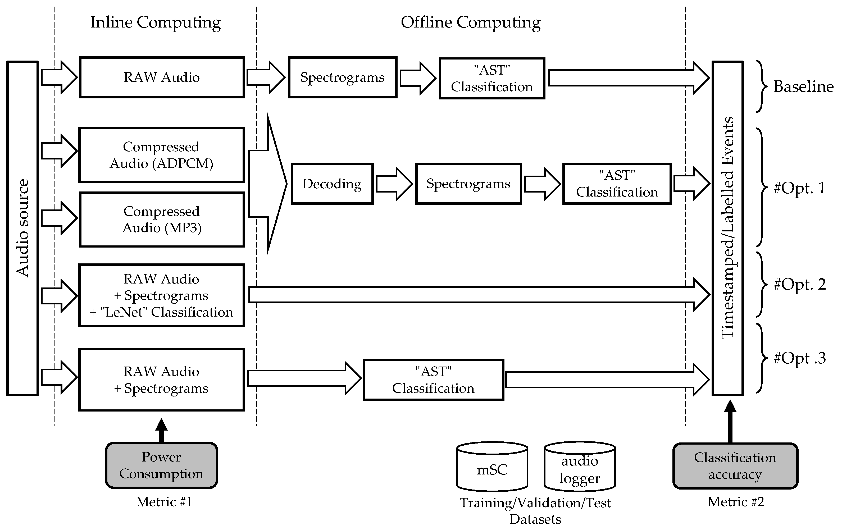
In this section, we present the approaches to balance the embedded CPU computing and storage activity. On the one hand, moving computing at the edge can help in reducing the amount of data to store onboard. However, edge computing is limited in both computing capability and embedded energy. On the other hand, we can reduce the load on the embedded CPU by shifting heavy computations to an offline server. In this case, more data must be stored onboard to allow the subsequent external classification process to produce useful results. Figure 1 illustrates the different approaches that we investigated to balance the computation load and storage activity at the edge. All approaches share the same audio front-end, meaning that audio samples are available in the logger memory buffers before any inline computing commences.

Figure 1.
Approaches to event timestamping.
2.2. Baseline Application
The baseline application, shown at the top of Figure 1, is used as a reference to evaluate three other options (namely #Opt1, #Opt2 and #Opt3). In this baseline application, the logger stores raw audio data with no additional computing over the entire deployment period. The offline system later computes spectrograms from the stored data (audio transient waveforms) and performs the classification. Because classification is performed offline, there are neither real-time, power, nor CPU constraints. In this case, classification can be performed using a complex model to reach higher accuracy, such as state-of-the-art Audio Spectrogram Transformers, referred to as “AST”.
2.2.1. Inline Compression (#Opt1)
Our first attempt (#Opt1) to reduce the logger power consumption by lowering mass storage activity is to apply an inline audio data compression. As a result, the server must decode the so-encoded data to reconstruct audio information before computing the spectrograms. We evaluate both ADPCM and MP3 compression algorithms, providing two distinct cases of compression ratio versus CPU requirements. The same AST model as for the baseline application is used for event classification, but model training is performed using altered datasets, obtained after encoding/decoding audio clips from the regular dataset. Doing so achieves a compression-aware training.
2.2.2. Inline Inference (#Opt2)
The second idea (#Opt2) is to move the entire classification process to the edge, allowing for a dramatic drop in the amount of data to be stored. In this case, the logger performs real-time spectrogram and classification computations on the audio stream. This results in drastically reduced storage activity and removes the need for any form of offline computing. Here, the classification process is constrained by the tightly limited computational power of the logger. In this case, the classification engine is based on a light model, referred to as “LeNet”, which will be detailed later on.
2.2.3. Inline Data Preparation (#Opt3)
The third initiative (#Opt3) presents an “in-between” approach where only feature extraction is performed on the logger, with spectrograms stored on-board for later offline classification. AST classification model is used for offline inference, with a training pipeline adapted to the inline computed spectrogram format.
2.3. Metrics
For concept proofing, we used a reduced keyword spotting (KWS) case study. The classification engine is trained using the freely available “mini Speech Commands” (mSC) dataset. It is a subset of the widely used “Speech Commands” dataset [20]. This public dataset consists of 8000 one-s-long audio files divided into eight classes (i.e., words to identify, namely: ’yes’, ’no’, ’up’, ’down’, ’left’, ’right’, ’go’ and ’stop’). We split the mSC dataset into three subsets for training, validation, and testing. In addition to the publicly available audio clips, we created an independent test set with our actual logger records consisting of 400 one-s-long labeled clips (50 clips for each class). In the following, we refer to the latter as the “audiologger” dataset.
As previously stated, we focus our study on two metrics. The first one is the logger autonomy. The options presented above are therefore compared in terms of power, obtained by measuring supply currents on real hardware during activity. The second metric relates to classification accuracy (i.e., the “usefulness” of the results). As already stated, each approach uses its own classification model, and comparing the performance of these models is not straightforward. By nature, audio is a continuous stream of information. In our case study, the models take discrete 1-s audio frames as input. However, audio events can be cut when slicing the audio into 1-s frames. Hence, to avoid missing audio events, a common practice is to run inferences on time-overlapping spectrograms [21]. Figure 2 illustrates this idea. With no prediction overlapping, inferences are performed on frames and , each having half of the audio event of interest (a ’yes’ keyword in this example) making the detection more likely to fail. With a 50% prediction overlapping, we can expect a correct detection on the newly added inferring frame . In this case, classification results obtained on previous () and next () frames can even help assess audio event start and end times more precisely [22], which can be crucial depending on the biologging application.

Figure 2.
Prediction overlapping.
This technique is trivial to implement with offline classification and does not impair the logger’s autonomy because the amount of spectrogram data to produce remains the same. However, as overlapping increases the inference rate, it is barely feasible with online classification (#Opt2) because of the limited computing power available onboard. In the best case, if the real-time constraint is not a limiting factor, the increased CPU activity results in increased energy consumption. In the context of this study, we do not investigate this application-specific inference overlapping parameter. Instead, we rely on the model’s accuracy on the audiologger dataset one-s-long clips as a common evaluation metric across all approaches.
3. Baseline Application Background
Our reference case (baseline application) is built upon previously reported work [19]. Considering either the audio recorder or the classification model and training datasets, this section summarizes the key matter that is required for the understanding of subsequent developments.
3.1. Data Collection
In this application, the logger records and stores unprocessed raw audio samples. All subsequent feature extraction and event classification is performed outboard, with no constraints on computational resources, external power consumption, or execution speed.
Hardware Architecture
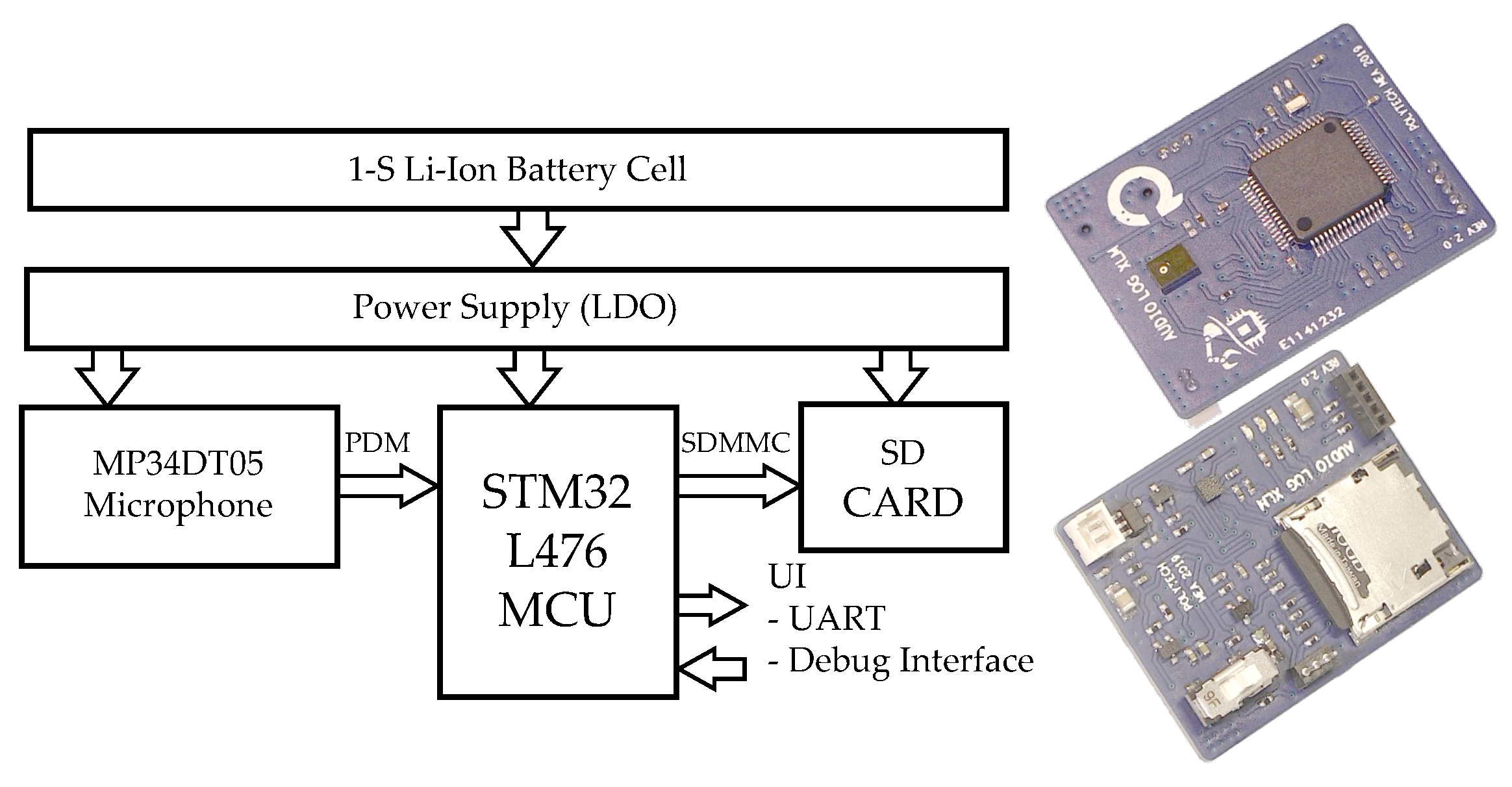
Figure 3 shows the hardware architecture of the audio logger. It is a minimalistic architecture designed around off-the-shelf electronic components with a low-power microcontroller that streams audio samples from a MEMS-digital-integrated microphone to an SD-Card.

Figure 3.
Audiologger hardware architecture.
The microphone output is a continuous digital Pulse Density Modulated (PDM) stream coming from an embedded modulator. Since a logger typically records months of audio signal, resulting in the production of tens of gigabytes of data, the choice of an SD-Card as storage media is obvious. The Micro-Controller Unit (MCU) then only handles data transfer from the microphone to the SD-Card with a buffering strategy that optimizes low-power states. We selected for this purpose the STM32L476, a high-end energy-efficient MCU, for the availability of dedicated hardware interface peripherals for both the microphone and the SD-Card. This MCU is designed around an ARM Cortex-M4 core, featuring a hardware Floating Point Unit (FPU). Further details on hardware choices are provided in [4].
The MCU Digital Filter for Modulator (DFSDM) peripheral drives the microphone modulator with a 2 MHz clock and performs PDM demodulation using a hardware-dedicated decimation filter. Audio quality (i.e., sampling rate and dynamics) is tuned at DFSDM level. In our case study, the decimation filter oversampling ratio is set to 32 with 24-bit data output obtained after summing every eight filter outputs. This results in a 7812 Hz audio sampling frequency. It is a low-sampling frequency with respect to usual digital audio standards, but sufficient for most biologging applications where the high-end audio spectrum does not contain relevant information. Audio samples are buffered into RAM by a Direct Memory Access (DMA) controller thus making the audio capture entirely hardware with no CPU software requirements. As a consequence, for the baseline application, the CPU is only involved in two tasks: (i) Applying a 16-bit roundoff on audio samples and (ii) Sending data onto mass storage in a user-friendly, directly playable format (Microsoft® raw audio WAV files).
3.2. Software Tuning
It is common knowledge that digital electronic power consumption is directly related to the operating frequency. When no CPU task needs to be performed, i.e., the system is only collecting samples, and the MCU is put in a sleeping state. To save energy, the main MCU clock is reduced to the lowest possible frequency so that the required peripherals still operate while the CPU clock is gated off. When software processing is required, the question of optimal clock frequency arises. Faster CPU leads to higher power consumption, with a proportionally reduced processing duration making the total energy requirement for a given task something nearly constant as one would first guess. Yet, hardware side effects such as: (i) the tuning of the FLASH memory latency, (ii) the consequence of using higher current less-efficient voltage regulators or (iii) the activation of internal PLL to speed up CPU operations produces non-linearities in the MCU power efficiency response to the clock frequency. Figure 4 highlights this idea with two fictive configurations.
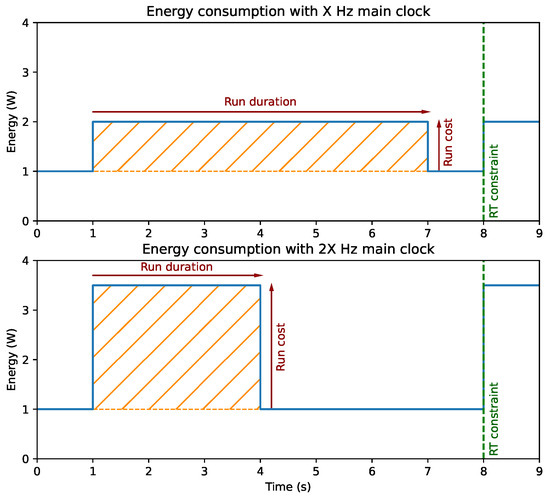
Figure 4.
Effect of CPU clock frequency on task execution and power efficiency.
In the upper scenario, the main clock is set to an arbitrary frequency of X Hz. At t = 1 s, the system awakens from its sleeping state and starts processing data for six ss. Upon completion, the system returns to sleep until the next Real-Time (RT) constraint for one second. In Figure 4, the orange-hatched area represents the energy overhead associated with the processing: W.s (or approximately 1.7 mW.h). In the lower scenario, the clock speed is doubled to 2X Hz. Under this new condition, the same task sees its processing duration halved. However, in this case, the processing energy overhead is W.s, worsening the logger autonomy.
The CPU clock frequency can be freely and dynamically adjusted to the most energy-efficient speed as long as RT constraints are met, e.g., in this example, the processing is completed by t = 8 s. Since clock frequency and processing time are proportional, energy efficiency is achieved when the ratio between run cost and clock frequency, i.e., energy spent per Hz, is minimized. We measure this ratio in our application for each clock speed ranging from 4 MHz to 80 MHz. Subsequently, each configuration presented in this paper runs at the most energy-efficient available speed. In the case of the baseline application, since little processing is required, the lowest frequency is selected.
3.3. Audio Events Classification
The AI classification is a two-step process that consists of converting input data into features, and then applying those features to a trained deep-learning model. As we already discussed our strategy concerning training and testing datasets, this section only covers data preparation and model choices.
3.3.1. Deep-Learning Model
Deep-learning-based audio classification can be achieved through two methods, depending on the model input data format: Time-domain audio samples or time-frequency-domain spectrograms [22]. We based our classification approach on the latter, which achieves state-of-the-art performances using Audio Spectrogram Transformer (AST) architectures [17]. This type of architecture was originally designed for natural language processing [23]. More recent works have adapted the approach for image classification [24] resulting in Vision transformers. The model we use is a readily available tuned version of a pre-trained Vision transformer. Pre-training was performed on large image datasets such as ImageNet [25], and then tuned for audio spectrogram processing with AudioSet [26].
We further fine-tuned this model for our downstream application using the “mini Speech Commands” (mSC) dataset.
3.3.2. Data Preparation (Spectrograms)
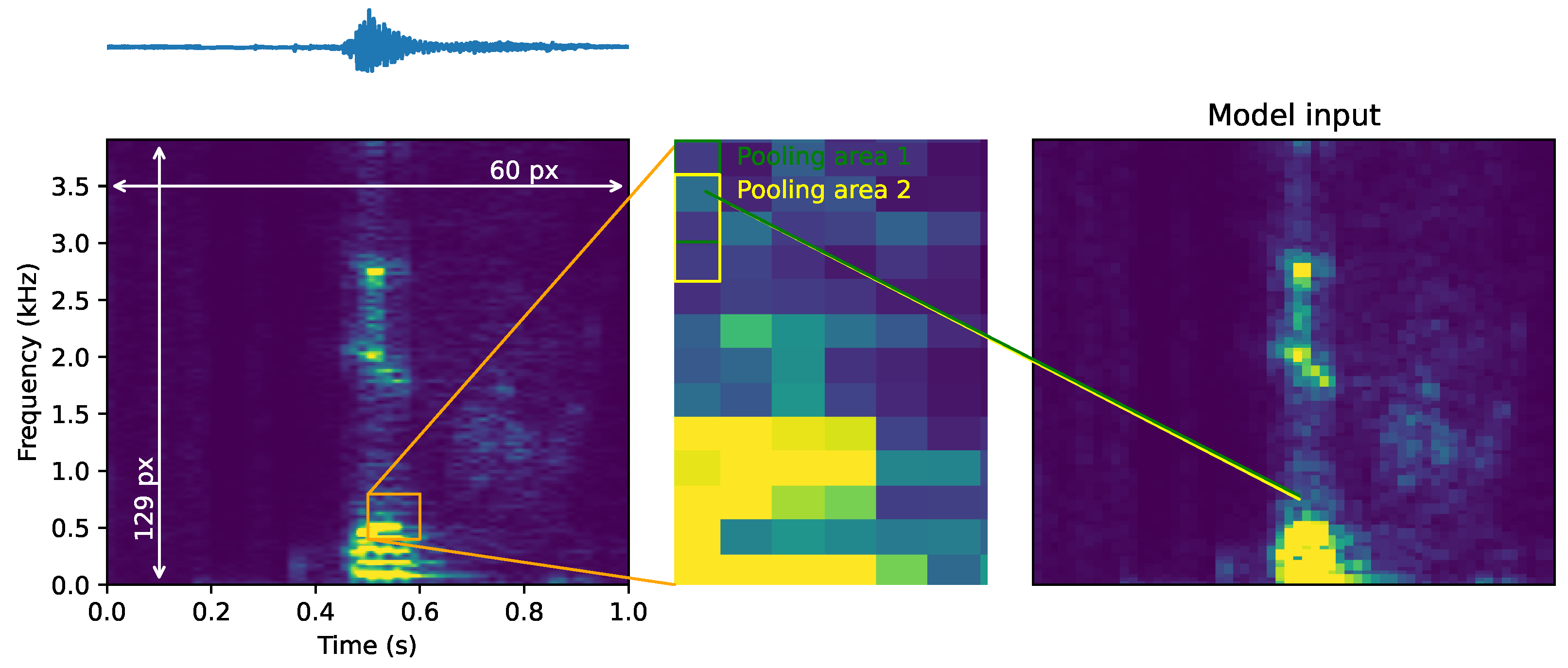
The mSC dataset is published in the form of 16 kHz, floating-point waveforms. To match the sampling specifications of our logger, and therefore the audiologger dataset, we first resampled mSC audio clips to 7812 Hz, 16-bit integers format. FFTs are then computed on 256-sample-long windows providing 129 frequency bins each. With a 50% overlap on these windows, about 1 s of audio source leads to a 60 × 129 pixels spectrogram. Following the advice provided in [17], spectrograms from mSC and audiologger dataset are normalized in terms of mean value and standard deviation. These parameters have been reported to be environment-specific [27], and should be computed logger-wise.
After this mSC and audiologger dataset alignment, a one-dimensional maximum pooling over the frequency axis is applied to improve the model’s generalization capabilities [28]. With a unity stride, we tested multiple pooling sizes ranging from one to four, with three giving consistently better results (see Figure 5).

Figure 5.
Spectrogram preparation and pooling.
4. Optimization Attempt #1: Inline Compression
An obvious way to reduce the amount of recorded data is to apply audio compression on recorded samples prior to storage. We considered two compression algorithms for this task. ADPCM encoding is a lightweight, lossy compression scheme that encodes the difference between two consecutive audio samples using four bits. This results in a 4:1 compression ratio. Note that an uncompressed audio sample (16-bit) is stored every 505 samples to prevent long-term drifting, thus slightly lowering the compression ratio. MP3 compression removes frequency-masked sounds and produces output using the Huffman encoding. This algorithm offers higher compression ratios than ADPCM at the cost of increased processing requirements. In this work, MP3 encoding is implemented with the help of the Shine library [29] providing a 16:1 compression ratio.
After decoding data into an audio transient waveform, the classification process is the same as that presented in Section 3. By definition, lossy compression algorithms introduce audio artifacts that may impair the classifier’s performance.
Figure 6 presents the effect of encoding/decoding on a 1s-long audio clip containing a ’yes’ keyword. The first panel represents the spectrogram computed from an original, uncompressed audio clip. The s spectrogram is obtained after applying MP3 encoding and decoding on the same clip. Differences in so-obtained spectrograms are better revealed on the third panel (pixel-wise subtraction).

Figure 6.
Waveform deformation induced by encoding/decoding on excerpt of a “yes” keyword waveform.
To account for spectrogram alteration due to compression, the deep-learning model fine-tuning is performed with spectrograms obtained using encoded/decoded audio clips from mSC and audiologger datasets. Note that encoded/decoded datasets are produced offline, yet use the very same software library as that used in the logger firmware.
5. Optimization Attempt #2: Embedded AI
Deep learning is computationally complex and its integration into energy-constrained systems remains challenging [30]. Yet, considering that inference on a short audio window produces a single few-bit encoded classification result, we can think of it as a highly destructive algorithm with a huge compression ratio.
Several DL models have been reported over the last years that are easily tweakable for audio recognition. For instance, let us mention LeNet-5 [31], ResNet [32], and MobileNet [33], which can all be either trained or fine-tuned for spectrogram classification. However, all these architectures have been developed mainly for mobile appliances with comfortable CPU power. In our case, a model’s computational complexity is not only limited by available power on-board, but must also meet a hard real-time constraint. As a matter of fact, embedded audio classification implies that an inference over a one-s audio clip is performed in less than one s, leaving margin for other CPU tasks including data preparation (spectrograms) and casual logger management tasks.
Considering our logger MCU, possible CPU frequencies range from a few MHz to 80 MHz. Even at full speed, none of the above reported models (no need to mention AST which does not even fit into memories) would pass the real-time constraint. For example, LeNet-5 architecture takes 2.6 s to infer a spectrogram at full speed.
Based on these observations, we designed two specific DL models that may be considered simplified versions of LeNet-5. We kept the idea of two consecutives CNN layers because it has consistently shown good results in the literature [34]. The first “light” model has been designed with energy efficiency in mind, while the second “heavy” architecture focuses on the maximum achievable accuracy within our context of limited resources. We used TensorFlow as the design framework for that purpose and its inference engine TensorFlow Lite for Microcontrollers [35].
To train the model (offline) with the same data representation as in the audio logger, the audio clips from the mSC dataset have been first resampled at 7812 Hz and quantized to 16-bit signed integers. Spectrograms are then computed using the Kiss FFT [36]. This FFT implementation has been retained for both its low-memory footprint and its ability to cope with 16-bit integer input samples. FFTs are performed over non-overlapping 128-samples-long audio frames (16.385 ms) so that a one-s audio clip translates into a pixels spectrogram. Note that overlapping audio frames is a widely used technique for performance improvement [37] that we used in Section 3. Yet, by increasing the spectrogram time resolution, we would also increase the CPU load for all subsequent processing steps (including inference).
Lower frequencies are noisy depending on the recording conditions, which tends to affect the performance of the CNN architecture. To mitigate this while reducing the required computing power, we discard the five lowest bins of each FFT, therefore reducing each spectrogram to a pixels array. Using a single precision 32-bit floating point representation for each pixel, one spectrogram occupies 14,640 bytes of memory.
5.1. Energy-Efficiency Driven Model
The first model was designed for a minimum accuracy threshold of 50% on the audiologger dataset classification with energy efficiency in mind. This model is depicted in Figure 7.

Figure 7.
Simplified LeNet-5 architecture.
The sheer amount of input data has a linear impact on the total inference time. Therefore, the earlier the data dimension is reduced in the process pipe, the stronger the impact on execution time. A computationally effective way to reduce dimension in audio classification tasks is to apply a pooling strategy [28]. Here, an aggressive version of this strategy is implemented using a subsampling layer applied directly to the input data, with no overlap. This is a simple dimension reduction mask that keeps the maximum pixel over an area of four, thus reducing the spectrogram picture to pixels. Next, the normalization layer is included to prevent overfitting. This layer has a very small impact on inference time (less than 1%). In the original LeNet-5 model, the first convolutional layer uses a kernel with a stride of 1. Instead, we used a kernel with no overlap (i.e., strides = 2). This combination accelerates calculations by a factor of nine on this single layer and reduces output dimensions for all subsequent layers. The price to pay is a drop in accuracy that remains within specifications. The following layers, including the s 2D convolution layer, the fully connected 32-neuron layer, and the final decision layer (eight neurons), are inspired by the LeNet-5 model with sizing driven by accuracy. Quantizing these parameters to 8-bit integers is a common practice when targeting resource-limited MCUs, as it allows for both RAM usage reduction and faster computing. In our case, the Cortex-M4 CPU features a hardware Floating Point Unit, making the calculation no slower with real numbers [38]. In addition, we measured a loss in accuracy of 13% when using 8-bit quantized weights. This is not surprising considering the aggressive simplifications performed on the model. For these reasons, the initial floating-point representation of model parameters was retained.
The deployment of the trained DL model onto the MCU is done with the help of the TensorFlow lite for Microcontrollers library available as C++ source code. The complete library has a code memory footprint of about 480 kB, yet including only the required subset to run inferences on our model, that footprint drops to only 80 kB. Data preprocessing (i.e., calculation of spectrograms) is easily ported to MCU since it was coded for that purpose in the first place. Yet, samples are now streamed from the microphone through the DFSDM/DMA hardware pipe. As explained earlier, an FFT is processed every 128 collected samples, resulting in 65 bins. By dropping five bins representing noise at low frequencies, a spectrogram column is obtained. After 61 repetitions of this process, the spectrogram is forwarded to the inference engine. The prediction result is finally encoded and stored in RAM, waiting to be written on the SD-card.
5.2. Accuracy Driven Model
The second model designed for MCU-based inference is driven by the RT constraint, i.e., less than 1 s inference time, with the CPU running at full speed (80 MHz). This new paradigm allows investigating more computationally complex models. Yet, complexity does not always bring good accuracy, so that among several candidates, only the model providing the better accuracy was retained. Figure 8 provides details on the architecture of the so-designed model.

Figure 8.
Upscaled model architecture for embedding.
Starting from the above model, we found that increasing the complexity for hopefully better results was not possible. This is not because of inference time going above RT limitations, but rather because of the limited memory amount that is available to run inferences (arena size). For completeness, note that only 75 kB of RAM, among a total of 128 kB, is available for the inference engine, accounting for complete logger needs.
6. Optimization Attempt #3: Inline Data Preparation
In this section, we move to the edge part of the classification process. As a matter of fact, the first data preparation stages exhibit an interesting balance between CPU requirements and opportunities for data dimension reduction. Data preparation mostly consists of the transformation of transient audio data into spectrograms. In the model presented in Figure 7, the first pooling layer can be considered as an additional data preparation step, movable outside of the trained engine. In doing so, the actual DL model starts with the normalization step (which does not offer any data reduction) of a downsized spectrogram computed and stored at the edge. We can think of this idea as an audio compression that destroys actual audio in the process but builds a highly compressed ML-friendly representation of the original information. Inferring remains an offline process, performed on high-end systems with neither RT nor power constraints. This brings the AST model back into the scene.
The DL model previously introduced for the baseline application uses pooling to improve model generalization capabilities, with a minimal stride of one because reducing the data dimension is of no particular interest when done offline. Now moving the data preparation to the edge, data reduction becomes the primary concern. To achieve higher data reduction, we remove pools overlapping, as done in the “light” model presented in Figure 7 (stride = pool size).
Several pooling strategies are available for audio classification: x-pooling along the time axis, y-pooling along the frequency axis, or a combination of both. Each impacts the classification accuracy [28]. The only parameter affecting the overall embedded system consumption is the pool stride (now same as pool size), as it reduces the amount of data to be stored.
To compute an equivalent compression ratio, let us first consider the case of a unity pooling size (i.e., full non-overlapped FFT spectrogram). In this case, 256 16-bit audio samples are converted into 127 frequency bins. Arbitrarily using 8-bit quantized FFT magnitudes, we roughly achieve a 1:4 compression ratio, equivalent to the ADPCM-encoding algorithm. Consequently, this idea has few benefits without considering larger pooling sizes.
A pooling with size four is achieved by considering either: (i) four consecutive bins in a single FFT (vertical mask of ) or (ii) four bins of the same frequency over four consecutive FFTs (vertical mask of ) or (iii) two consecutive bins of the same frequencies over two consecutive FFTs. The latter is done in Section 5 (mixed pooling of ). Using either pooling of size four, the compression ratio is equivalent to that obtained with MP3 encoding (1:16).
We also considered a larger pooling size of nine, achieved by mixing frequency and time pooling () as pooling over only one dimension this long is unrealistic. In this case, the compression ratio reaches 1:81.
7. Results
We implemented the three above-discussed attempts to reduce power consumption. This section presents results obtained on each one in two parts, corresponding to the two established metrics, namely the embedded power consumption and the AI performance. First, we only consider the impact of each onboard implemented algorithm energy-wise, and second, we discuss the subsequent classification accuracy.
7.1. CPU Energy Efficiency
As already discussed, the MCU power efficiency depends on clock settings, with a non-linear relationship due to the contribution of differents internal hardware resources at various speeds. In order to measure the CPU energy efficiency, i.e., the energy spent per clock MHz, we profiled transient currents in our application with clock frequencies ranging from 4 to 80 MHz by using a Keysight CX1102A current probe and a CX3324A waveform analyzer. From this, we deduce the energy overhead that results from activating CPU (i.e., running software), as defined in Section 3.2.
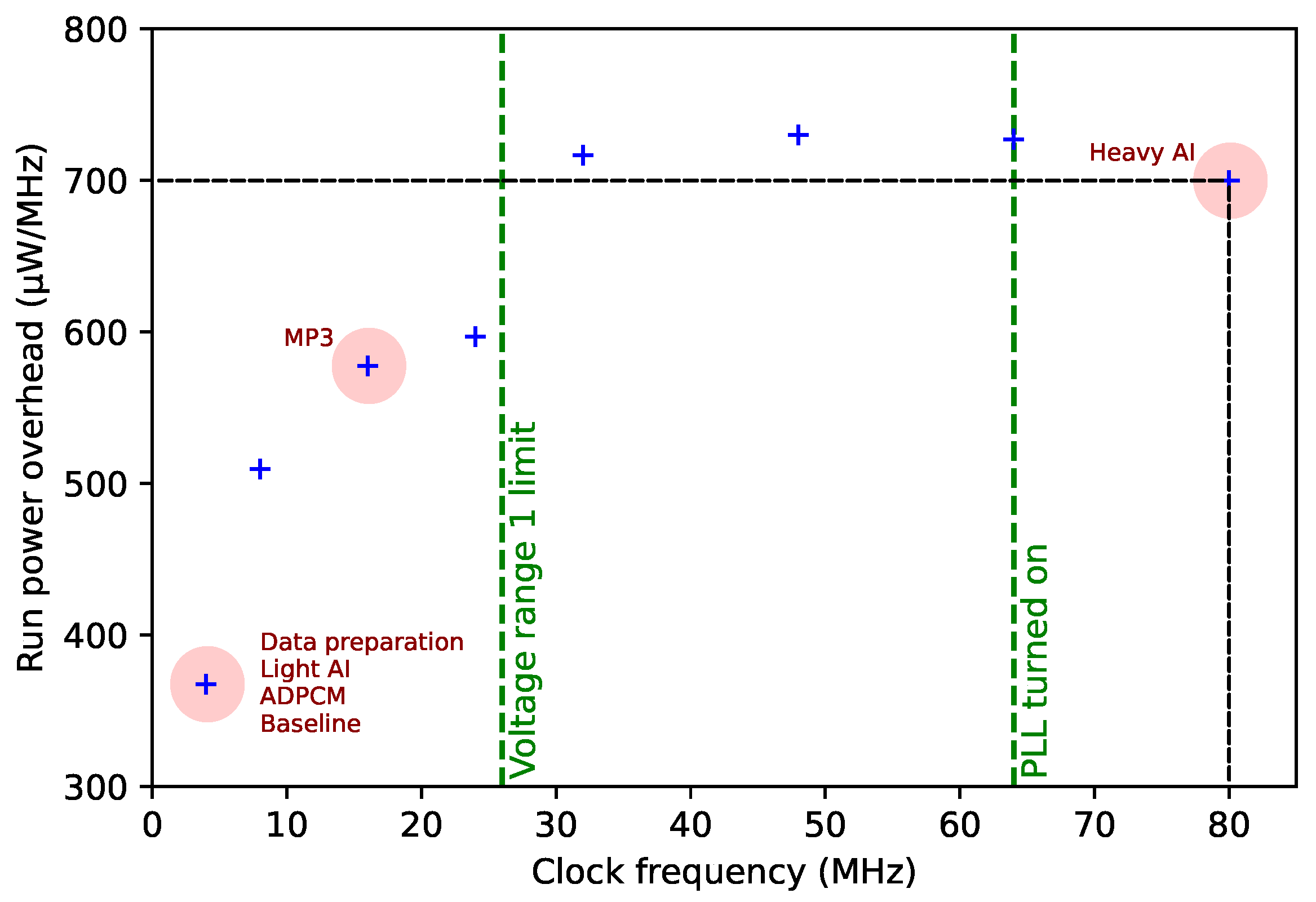
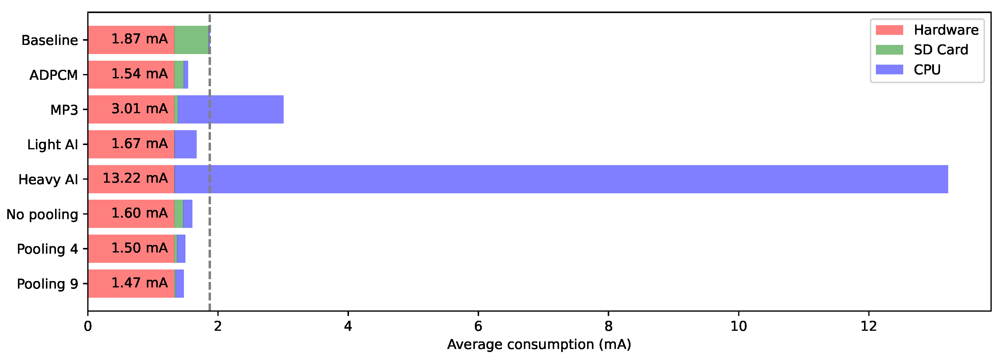
Energy cost tends to increase along with clock frequency. When running in the lower frequency range (<=24 MHz), energy efficiency is achieved by reducing clock speed as much as allowed by the computation load. If the RT constraints cannot be met below this threshold, then the preferable option is to push the clock speed to the maximum frequency (80 MHz). Most of the embedded algorithms presented in this paper can meet their RT constraints using the lowest and most efficient clock speed. The two exceptions are the MP3 requiring 16 MHz and the “heavy” embedded AI model requiring the full 80 MHz speed. Compared to the baseline 4 MHz clock speed, the two latter configurations, respectively, draw 57% and 90% more energy per MHz. Note that the “heavy” AI model would meet all RT constraints at 64 MHz but would in this case require 100% more energy than the one of the baseline application, so that there is no benefit in reducing the clock speed.
Figure 9 reports the measured power overhead per clock MHz (crosses) and corresponding setpoint for each embedded approach discussed in this work.
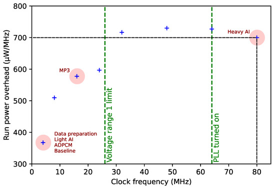
Figure 9.
Frequency-relative run power overhead vs. clock frequency and selected operating frequencies for the different involved algorithms.
7.2. Embedded Power Consumption
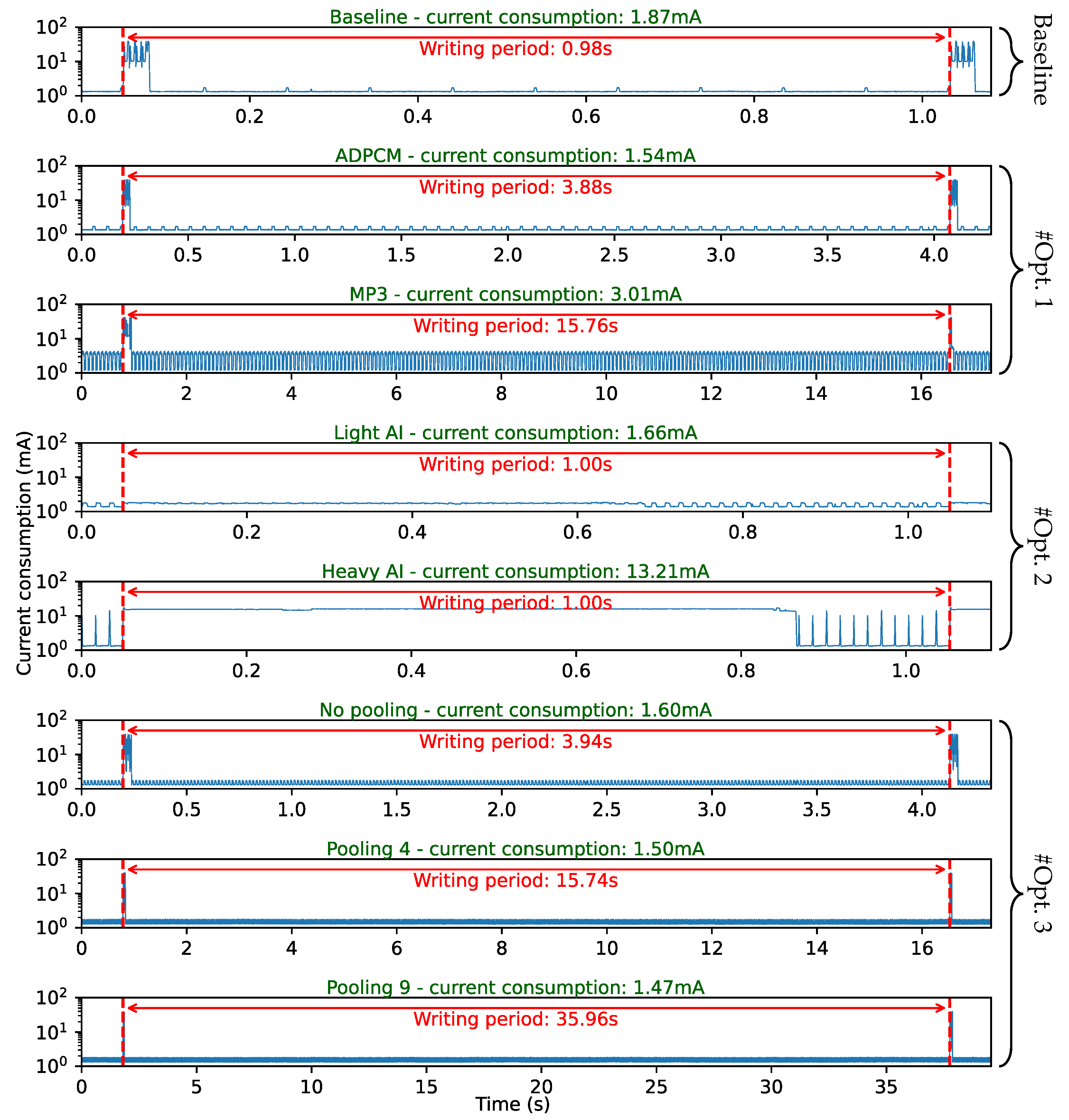
In order to compare their energy consumption, each scenario has been fully implemented on the logger and the transient supply current has been captured using the same setup as above. Figure 10 presents the obtained transient currents, measured from a 4.2 V supply voltage (mimicking a single-cell Li-Ion battery) during logger recording. Note that the time scale differs from one scenario to another in order to display resulting current over a complete operation cycle for each case.
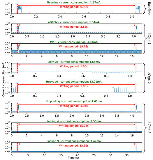
Figure 10.
Total transient currents measured on the real audiologger during a complete cycle of data collection and processing for the different scenarios.
Higher current peaks correspond to SD writing events. In a previous study [4], it was observed that SD writing power efficiency improves when large data chunks are stored at once. Therefore, data are always buffered prior to SD writing, with a constant buffer size of 30 SD sectors (15 kB). This buffer is the same for all scenarios, therefore the period between writing events directly depends on the data reduction ratio. In the case of the baseline application, very little CPU energy is required to manage buffers between writing events that occur every 0.98 s.
In the #Opt1 attempt, when using ADPCM, CPU activity becomes slightly noticeable, while writing events frequency is divided by 4. ADPCM encoding occurs every 11 ms for 65 ms processing time. Note that the CPU runs at 4 MHz clock speed because no heavy calculation is involved. MP3 diminishes writing operations even further (1:16 with respect to the baseline application). Yet, CPU activity is quite noticeable in this case, with compression algorithm invoked every 74 ms for 47 ms processing time. Here, real-time constraints and the complex MP3 algorithm involve faster CPU clocking (16 MHz) thus increasing overall power consumption.
The inline classification used in #Opt2 obviously places high demands on the CPU, specifically with the “heavy” DL model that results in power consumption one order of magnitude above that of the baseline application. Still, when using the “light” model version, the power consumption is lower than that required for MP3 encoding. This configuration even allows for 11.8% energy saving with respect to the baseline reference.
#Opt3 mostly involves FFT computations, and we can neglect the pooling processing time and its effect on power consumption. It is evidenced that larger pool sizes lead to higher data reduction ratios, and thus storage energy savings. In our case, the most energy-efficient variant is obtained with the higher pooling size ().
Figure 11 summarizes the logger average power consumption for each scenario. From left to right, uncompressible onboard hardware contribution, including power regulation stages, microphone, and audio data buffering is displayed first (red). Then comes the data storage cost (green), and finally the CPU overhead (blue).
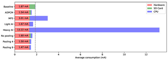
Figure 11.
Consumption per component.
7.3. Audio Events Classification
For #Opt2, both embedded models were trained using the Tensorflow framework, whereas offline AST models (Baseline, #Opt1, and #Opt3) were fine-tuned with the Pytorch framework. The models are trained using train and validation sub-dataset from mSC dataset, and training was halted when no improvement was observed on the validation subset for 20 consecutive epochs and best weights were restored. Finally, we assess the generalization capabilities of the trained model by comparing accuracy results on the test subset and audiologger dataset. This step also helps detect a potential domain mismatch between the two datasets [39]. Table 1 only presents accuracies obtained on the audiologger dataset.

Table 1.
Accuracy results on audiologger dataset.
We observe that AST models significantly outperform CNN models. This is expected since: (i) they achieve state-of-the-art spectrogram classification accuracy and (ii) there are no constraints on calculation resources. Transformer models require fewer epochs to train (<30) than their CNN counterparts, yet each epoch takes longer to compute.
Compared to the model inferring spectrograms based on raw waveforms, using compression (ADPCM and MP3) and non-overlapping FFT windows (no pool) produces a slight decrease in accuracy. Note that classification would work without fine-tuning with encoded/decoded training sets. However, accuracy would drop to 89.75% and 78.25% for ADPM and MP3, respectively.
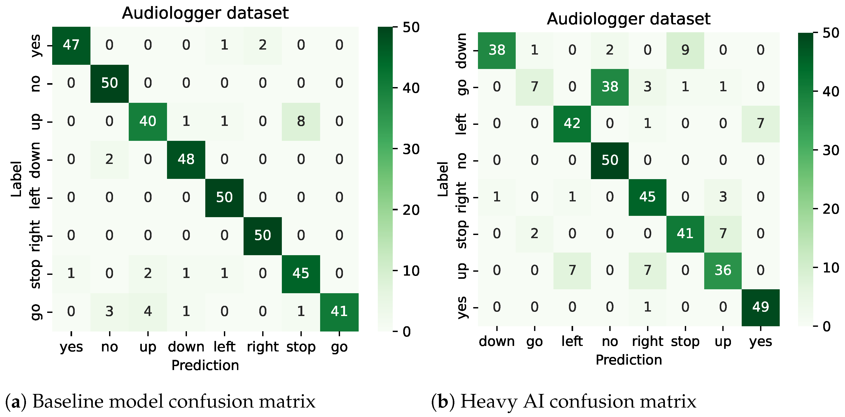
Both embedded DL models (#Opt2) do not excel regarding accuracy with only 77% and 51.25% classification success for the “heavy” and “light” versions, respectively, as expected. One can consider that 77% accuracy is the best result we were able to obtain at this moment, on keyword spotting task, when running full speed on a general-purpose low-power 32-bit FPU microcontroller. To better analyze the information loss with the “heavy” embedded model, its confusion matrix presented in Figure 12b can be compared to that of the baseline application Figure 12a. Both are produced using the audiologger dataset. While the AST model exhibits fairly high-accuracy results consistently across all classes, we notice that the CNN model fails to identify some classes such as the “go” keyword or less obviously the “up” keyword. These flaws severely impair the model’s utility in the context of biologging since it may bias the analysis of animal behavior. Such accuracy inconstancy across classes is expected with DL classification and may come from several factors including training dataset, training parameters, and the model itself. It is worth noting that the accuracies obtained on the same classes with AST classifier are also below those of other classes, confirming that these particular classes are challenging to identify. There is no general conclusion to draw here, as poor accuracy on a specific class is basically application dependent. In case of a no-go, one should consider improving the dataset.
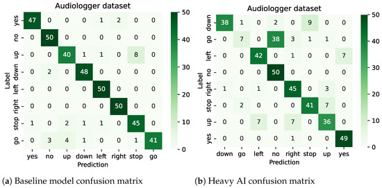
Figure 12.
Confusion matrices comparison on audiologger dataset for both baseline model and heavy AI.
When implementing inline feature extraction (#Opt3), the obtained results show that data trimming (i.e., larger pool sizes) can be performed without any noticeable drop in performance. Model success is even improved using non-overlapping frequency-pooling (from 85.5% to 89%). With no pooling, model accuracy can be improved by offline post-processing of the spectrograms to apply the same pooling and striding strategy as in the raw waveform model (then increasing accuracy up to 91.47%). Finally, considering larger pool sizes (), AST model’s accuracy drops to 76.25%, showing the limits of the data reduction achievable by the #Opt3 approach (1:16, same as MP3).
8. Discussion
Considering to the above results, we can now identify the best option. If we sort our attempts upon accuracy results, the #Opt2 attempt fails to reach acceptable levels. In fact, it seems challenging to obtain AST accuracies within limited computational resources. Regarding accuracy, we can also discard both “high-pool” and “pool-time” variants of the #Opt3 approach. Now considering the CPU overhead and related power consumption, the MP3 variant of #Opt1 is also eliminated.
Candidates that offer better energy efficiency than that of the baseline application, while preserving the accuracy of the classification are: (i) ADPCM compression within #Opt1 attempt, and (ii) two cases of #Opt3, using either “no-pool” or “frequency-pooling” variants. The former exhibits worsened power consumption as the one measured using ADPCM compression, and comes with the added cost of destroying listenable audio. Thus, we discard it.
Finally, we are left with two interesting options. Yet, the benefit in power consumption gained from shifting toward the computation of spectrograms as a way to reduce the storage energy seems inadequate considering the sacrifice of listenable audio data. In conclusion, at this moment, we would retain ADPCM compression as the best way to improve the logger autonomy, with negligible loss of information.
There is another benefit of using offline AST classification, because ASTs are already trained, these models only need few additional pieces of information to be fine-tuned for a specific application, which makes the approach significantly more interesting for biologging research, and the availability of application-specific self-recorded small datasets. This is not the case for our CNN architectures, which require larger dataset for complete training from scratch. For instance, using the same AST as for the baseline application, and using the sole audiologger dataset with only 400 audio clips, split into three subsets for fine-tuning (240), validation (80) and test (80), we were able to reach 95% accuracy on classification results.
Reaching only 92.75% classification accuracy on raw audio is underwhelming compared to recently reported state-of-the-art results. A reason is the low sampling frequency we use in the logger (7812 Hz) that not only destroys high-frequency information but also introduces aliasing artifacts known to impair machine learning algorithms [40]. Using the original 16 kHz mSC dataset, without down-sampling, for both fine-tuning, validation and testing, we obtained 96.75% accuracy.
9. Related Work
For offline classification, the AST model achieves state-of-the-art performances with 98.11% accuracy on the Speech Commands dataset, settling a new reference, previously held by a CNN-based architecture [41]. The AST architecture is attention-based and may be applied to varying input audio lengths. With excellent results obtained on several datasets, AST appears at this moment as a promising generic audio classifier [17]. However, AST models are both memory (~1GB) and computationally intensive. In addition, there is a strong demand for simple keyword-spotting solutions that are able to run on small embedded systems. The best comparison we can make with our work is to consider these applications, and therefore the cases of an embedded classification task.
Several studies have employed the Speech Command (SC) dataset since its publication [20]. The full SC dataset actually includes 35 keywords and several clips of background noises, yet several studies have been working on a subset including 10 classes (“on” and “off” being added to our mSC eight classes) alongside an “unknown” class that regroup other words from the full SC dataset, and a “silent” class representing background noise only, for a total of 12 classes. Below is a selection of related works using this dataset, that we can use to discuss our results.
The study reported in [28] demonstrated that DNN architectures could outperform Hidden Markov Models, which represented the state-of-the-art approach for keyword spotting at that time. The classifiers introduced here use 40 log-mel filter banks calculated on 25 ms-long frames with 60% overlap. For comparison with our work, we retain their tpool-2 model, a two CNN-layer deep architecture design with little constraints on computation, and their one-stride1 model, an architecture with a single CNN layer designed to run within a limited complexity budget.
In [42], the authors introduced the concept of residual architectures allowing training of deeper networks. In this work, audio is prepared by first applying a band-pass filter from 20 Hz to 4 kHz. Then, 40 MFFCs on 30 ms windows with 2/3 overlap are computed. From this study, we retain two architectures: (i) the best performing one res26, and (ii) res8-narrow designed to minimize computational complexity and memory footprint.
Finally, different architectures were explored in [43], with varying constraints on memory and computational resources. Feature extraction consisting of 10 MFCCs is performed on 40 ms windows with 50% overlap. Among proposed architectures, we retain the smallest CNN-S and heaviest CNN-L CNN-based models. Note that CNN-S is the least computationally complex model we were able to find in the literature, making the comparison with our work much more appropriate.
Table 2 compares our results with above-listed studies. For fair comparison, both our “light” and “heavy” models have been retrained to account for the 12 classes used in the literature. Furthermore, these models are trained, validated and tested with the sole SC dataset (i.e., our audiologger dataset is not used here). In this case, because no out-of-domain sample is used in the accuracy measurement, the obtained results are significantly better than those reported in Table 1 (from 51.25% to 76.1% and from 77% to 83.7% for “light” and “heavy” models, respectively). The comparison is based on computational complexity (represented by both input size, and the subsequent number of multiplications per inference), memory footprint (represented by the number of model parameters), and accuracy results. Direct comparison of power consumption is not feasible due to the variety of hardware platforms used in the literature, and the lack of reported results. Therefore, only the model complexity can provide clues concerning that matter.

Table 2.
Comparision of the heavy AI models with others models for small footprint keyword-spotting task. The comparison considers the input size of a model, the number of parameters, its total multiplication count for one inference, and its accuracy.
With less than two-million multiplications per inference, our “heavy” model is the simplest one by a consequent margin. As established in Figure 10, this model reaches our MCU capability limit. Regarding input sizes, the work in [43] achieves the best data reduction, with good accuracy results of the mSC, proving that few MFCCs perform well on this speech recognition task. Because bioacoustics applications address a wider variety of sounds, we choose to keep the frequency resolution obtained after FFT unaltered, and therefore avoid further reducing the input size. Since the model complexity is linearly correlated with the input size, we cannot explore more complex architectures, unless we accept higher power consumption. In [43], with 2.4M multiplications, the real-time inference is demonstrated on high-end MCU (Cortex-M7); however, this model would not meet our power consumption constraints. Studies focusing on mobile appliances [42] reach even higher accuracies, but the required computational power is an order of magnitude higher.
In summary, the application we address is highly constrained by model complexity. Furthermore, in the context of a generic solution for sound classification task, we prefer avoiding application-specific feature extraction approaches and consequently retain spectrograms for data preparation. In addition to these two limitations is the fact that when we work with low audio-sampling frequency. These constraints explain the 4% to 8% accuracy loss we observe with respect to the literature.
10. Conclusions and Future Work
In the context of biologging, and of IoT more generally, there is an increasing interest in employing embedded AI algorithms so that a large amount of information can be processed at the source. This results in reducing the costs of saving or transmitting the information.
In this paper, we take an audio recorder for wildlife monitoring as a case study. We explore different approaches to record audio data and to perform event classification. The first straightforward approach is to record raw audio data and perform classification on non-constrained hardware. Doing so allows for the highest classification accuracy results but comes at the cost of high-energy requirements on data storage.
In our first approach, we initially tried to tackle this issue by using inline audio compression. When chosen wisely, compression can significantly reduce storage activity. However, due to their lossy nature, such algorithms introduce noise leading to small, yet noticeably decreased classification accuracy. Both ADPCM and MP3 compression techniques were investigated with similar accuracy results. Taking the embedded power consumption into account disqualifies MP3 for this application due to the complexity of the algorithm and the subsequent load on the CPU.
In our second approach, we tried to implement the classification task at the edge with an expected dramatic reduction in the amount of data to be stored. While this approach indeed reduces storage activity to negligible levels, it is balanced by poor classification accuracy that results from limitations on deep-learning model complexity that we can run in real-time on a general-purpose low-power microcontroller. In fact, high-accuracy inference at the edge, relying on the sole speed of a standard processor core is not realistic if the logger autonomy comes first. One must wait for AI-dedicated, energy-efficient embedded solutions. Let us mention the Google coral chip, a powerful hardware inference accelerator that draws around 1.65 W [44]. This is two orders of magnitude above our audio logger power consumption.
Finally, we proposed computing and storing spectrograms at the edge, instead of transient audio, for later inference. By applying carefully crafted pooling strategies on the spectrograms, we were able to achieve a good compression ratio while still allowing for high-accuracy classification. The cost of this approach is the destruction of listenable audio.
In summary, regarding the main contributions of this work, we can mention that most reported results on audio classification in the literature are obtained using publicly available datasets. In this work, we used these public datasets for training only, while accuracy results were measured using our own audio clips, obtained from a real embedded bioacoustics recorder. Furthermore, we evaluated the performance of state-of-the-art classifiers when audio data have been compressed. The results show that compression-aware fine-tuning can prevent a 12% drop in accuracy with respect to MP3 encoding. To the best of our knowledge, this is the first time in the audio biologging field that deep learning classification is considered in the audio pipeline from the embedded energy perspective. We finally demonstrated that using inline data preparation in the context of DL classification for reducing data dimension and storage energy can be considered as an effective way to save power without compromising information.
Let us recall that the presented results are valid in the context of sensor nodes with onboard data storage. Considering communicating nodes and associated power costs may lead to a different conclusion regarding what option is the best for power reduction, with compression ratio becoming the primary issue. Future work might consider variants in the data preparation, such as using MFCC or Mel-Spectrograms for further data reduction, and explore non-supervised clustering approaches.
Author Contributions
Conceptualization, S.C.-J.; Methodology, L.L. and J.M.; Software, J.M.; Validation, S.C.-J., L.L. and J.M.; Writing, J.M. and L.L.; Supervision, S.C.-J. and L.L.; Project administration, S.C.-J. and L.L.; Funding acquisition, S.C.-J. All authors have read and agreed to the published version of the manuscript.
Funding
This research was funded by the Labex Cemeb (ANR-10-LABX-0004) and the Labex NUMEV (ANR-10-LABX-0020), by the REPOS project funded by the i-Site MUSE (ANR-16-IDEX-0006), and by the TERRA FORMA project (ANR-21-ESRE-0014).
Data Availability Statement
The model, source code and dataset can be downloaded at: https://gite.lirmm.fr/jmiquel/classification-biologging (accessed on 1 April 2023).
Conflicts of Interest
The authors declare no conflict of interest.
Abbreviations
The following abbreviations are used in this manuscript:
| ML | Machine Learning |
| DL | Deep Learning |
| MCU | Microcontroller Unit |
| MEMS | Micro-Electro-Mechanical System |
| PDM | Pulse Density Modulation |
| DFSDM | Digital Filter for Modulator |
| FPU | Floating Point Unit |
| RT | Real-Time |
| AST | Audio Spectrogram Transformer |
| mSC | mini Speech Commands |
| MFCC | Mel-Frequency Cepstral Coefficients |
References
- Hill, A.P.; Prince, P.; Snaddon, J.L.; Doncaster, C.P.; Rogers, A. AudioMoth: A low-cost acoustic device for monitoring biodiversity and the environment. HardwareX 2019, 6, e00073. [Google Scholar] [CrossRef]
- Beason, R.D.; Riesch, R.; Koricheva, J. AURITA: An affordable, autonomous recording device for acoustic monitoring of audible and ultrasonic frequencies. Bioacoustics 2019, 28, 381–396. [Google Scholar] [CrossRef]
- Whytock, R.C.; Christie, J. Solo: An open source, customizable and inexpensive audio recorder for bioacoustic research. Methods Ecol. Evol. 2017, 8, 308–312. [Google Scholar] [CrossRef]
- Miquel, J.; Latorre, L.; Chamaillé-Jammes, S. Addressing Power Issues in Biologging: An Audio/Inertial Recorder Case Study. Sensors 2022, 22, 8196. [Google Scholar] [CrossRef] [PubMed]
- Talla, S.; Ghare, P.; Singh, K. TBDRS: Threshold Based Data Reduction System for Data Transmission and Computation Reduction in WSNs. IEEE Sens. J. 2022, 22, 10880–10889. [Google Scholar] [CrossRef]
- Elsayed, W.M.; El-Bakry, H.M.; El-Sayed, S.M. Data reduction using integrated adaptive filters for energy-efficient in the clusters of wireless sensor networks. IEEE Embed. Syst. Lett. 2019, 11, 119–122. [Google Scholar] [CrossRef]
- Theodorou, T.; Mporas, I.; Fakotakis, N. An overview of automatic audio segmentation. Int. J. Inf. Technol. Comput. Sci. 2014, 6, 1. [Google Scholar] [CrossRef]
- Prince, P.; Hill, A.; Piña Covarrubias, E.; Doncaster, P.; Snaddon, J.L.; Rogers, A. Deploying acoustic detection algorithms on low-cost, open-source acoustic sensors for environmental monitoring. Sensors 2019, 19, 553. [Google Scholar] [CrossRef]
- Tuia, D.; Kellenberger, B.; Beery, S.; Costelloe, B.R.; Zuffi, S.; Risse, B.; Mathis, A.; Mathis, M.W.; van Langevelde, F.; Burghardt, T.; et al. Perspectives in machine learning for wildlife conservation. Nat. Commun. 2022, 13, 792. [Google Scholar] [CrossRef]
- Stowell, D.; Wood, M.D.; Pamuła, H.; Stylianou, Y.; Glotin, H. Automatic acoustic detection of birds through deep learning: The first bird audio detection challenge. Methods Ecol. Evol. 2019, 10, 368–380. [Google Scholar] [CrossRef]
- Xie, J.; Zhu, M. Handcrafted features and late fusion with deep learning for bird sound classification. Ecol. Inform. 2019, 52, 74–81. [Google Scholar] [CrossRef]
- Best, P.; Ferrari, M.; Poupard, M.; Paris, S.; Marxer, R.; Symonds, H.; Spong, P.; Glotin, H. Deep learning and domain transfer for orca vocalization detection. In Proceedings of the 2020 International Joint Conference on Neural Networks (IJCNN), Glasgow, UK, 19–24 July 2020; pp. 1–7. [Google Scholar]
- Jung, D.H.; Kim, N.Y.; Moon, S.H.; Jhin, C.; Kim, H.J.; Yang, J.S.; Kim, H.S.; Lee, T.S.; Lee, J.Y.; Park, S.H. Deep learning-based cattle vocal classification model and real-time livestock monitoring system with noise filtering. Animals 2021, 11, 357. [Google Scholar] [CrossRef] [PubMed]
- Bishop, J.; Falzon, G.; Trotter, M.; Kwan, P.; Meek, P. Sound analysis and detection, and the potential for precision livestock farming—A sheep vocalization case study. In Proceedings of the 1st Asian-Australasian Conference on Precision Pastures and Livestock Farming, Hamilton, New Zealand, 16–18 October 2017; pp. 1–7. [Google Scholar]
- Kim, T.; Lee, J.; Nam, J. Comparison and analysis of SampleCNN architectures for audio classification. IEEE J. Sel. Top. Signal Process. 2019, 13, 285–297. [Google Scholar] [CrossRef]
- LeCun, Y.; Bengio, Y.; Hinton, G. Deep learning. Nature 2015, 521, 436–444. [Google Scholar] [CrossRef]
- Gong, Y.; Chung, Y.A.; Glass, J. Ast: Audio spectrogram transformer. arXiv 2021, arXiv:2104.01778. [Google Scholar]
- Wang, Z.A.; Moustahfid, H.; Mueller, A.V.; Michel, A.P.; Mowlem, M.; Glazer, B.T.; Mooney, T.A.; Michaels, W.; McQuillan, J.S.; Robidart, J.C.; et al. Advancing observation of ocean biogeochemistry, biology, and ecosystems with cost-effective in situ sensing technologies. Front. Mar. Sci. 2019, 6, 519. [Google Scholar] [CrossRef]
- Latorre, L.; Miquel, J.; Chamaillé-Jammes, S. MEMS based Low-Power Multi-Sensors device for Bio-Logging Applications. In Proceedings of the 2021 Symposium on Design, Test, Integration & Packaging of MEMS and MOEMS (DTIP), Paris, France, 25–27 August 2021; pp. 1–4. [Google Scholar]
- Warden, P. Speech commands: A dataset for limited-vocabulary speech recognition. arXiv 2018, arXiv:1804.03209. [Google Scholar]
- Kons, Z.; Toledo-Ronen, O.; Carmel, M. Audio event classification using deep neural networks. In Proceedings of the Interspeech, Lyon, France, 25–29 August 2013; pp. 1482–1486. [Google Scholar]
- Stowell, D. Computational bioacoustics with deep learning: A review and roadmap. PeerJ 2022, 10, e13152. [Google Scholar] [CrossRef]
- Vaswani, A.; Shazeer, N.; Parmar, N.; Uszkoreit, J.; Jones, L.; Gomez, A.N.; Kaiser, Ł.; Polosukhin, I. Attention is all you need. In Advances in Neural Information Processing Systems; MIT Press: Cambridge, MA, USA, 2017; Volume 30. [Google Scholar]
- Dosovitskiy, A.; Beyer, L.; Kolesnikov, A.; Weissenborn, D.; Zhai, X.; Unterthiner, T.; Dehghani, M.; Minderer, M.; Heigold, G.; Gelly, S.; et al. An image is worth 16x16 words: Transformers for image recognition at scale. arXiv 2020, arXiv:2010.11929. [Google Scholar]
- Deng, J.; Dong, W.; Socher, R.; Li, L.J.; Li, K.; Fei-Fei, L. Imagenet: A large-scale hierarchical image database. In Proceedings of the 2009 IEEE Conference on Computer Vision and Pattern Recognition, Miami, FL, USA, 20–25 June 2009; pp. 248–255. [Google Scholar]
- Gemmeke, J.F.; Ellis, D.P.; Freedman, D.; Jansen, A.; Lawrence, W.; Moore, R.C.; Plakal, M.; Ritter, M. Audio set: An ontology and human-labeled dataset for audio events. In Proceedings of the 2017 IEEE international conference on acoustics, speech and signal processing (ICASSP), New Orleans, LA, USA, 5–9 March 2017; pp. 776–780. [Google Scholar]
- Bradfer-Lawrence, T.; Gardner, N.; Bunnefeld, L.; Bunnefeld, N.; Willis, S.G.; Dent, D.H. Guidelines for the use of acoustic indices in environmental research. Methods Ecol. Evol. 2019, 10, 1796–1807. [Google Scholar] [CrossRef]
- Sainath, T.N.; Parada, C. Convolutional neural networks for small-footprint keyword spotting. In Proceedings of the Interspeech 2015, Dresden, Germany, 6–10 September 2015; pp. 1478–1482. [Google Scholar]
- Beauxis, R. Shine: Fast Fixed-Point Mp3 Encoding. Available online: https://github.com/toots/shine (accessed on 1 April 2023).
- Merenda, M.; Porcaro, C.; Iero, D. Edge machine learning for ai-enabled iot devices: A review. Sensors 2020, 20, 2533. [Google Scholar] [CrossRef] [PubMed]
- LeCun, Y.; Bottou, L.; Bengio, Y.; Haffner, P. Gradient-based learning applied to document recognition. Proc. IEEE 1998, 86, 2278–2324. [Google Scholar] [CrossRef]
- He, K.; Zhang, X.; Ren, S.; Sun, J. Deep residual learning for image recognition. In Proceedings of the IEEE Conference on Computer Vision and Pattern Recognition, Las Vegas, NV, USA, 27–30 June 2016; pp. 770–778. [Google Scholar]
- Howard, A.G.; Zhu, M.; Chen, B.; Kalenichenko, D.; Wang, W.; Weyand, T.; Andreetto, M.; Adam, H. Mobilenets: Efficient convolutional neural networks for mobile vision applications. arXiv 2017, arXiv:1704.04861. [Google Scholar]
- Sainath, T.N.; Vinyals, O.; Senior, A.; Sak, H. Convolutional, long short-term memory, fully connected deep neural networks. In Proceedings of the 2015 IEEE International Conference on Acoustics, Speech and Signal Processing (ICASSP), South Brisbane, QLD, Australia, 19–24 April 2015; pp. 4580–4584. [Google Scholar]
- David, R.; Duke, J.; Jain, A.; Janapa Reddi, V.; Jeffries, N.; Li, J.; Kreeger, N.; Nappier, I.; Natraj, M.; Wang, T.; et al. Tensorflow lite micro: Embedded machine learning for tinyml systems. Proc. Mach. Learn. Syst. 2021, 3, 800–811. [Google Scholar]
- Mark, B. A Fast Fourier Transform (FFT) library that tries to Keep it Simple, Stupid. Available online: https://github.com/mborgerding/kissfft (accessed on 1 April 2023).
- Elliott, D.; Otero, C.E.; Wyatt, S.; Martino, E. Tiny transformers for environmental sound classification at the edge. arXiv 2021, arXiv:2103.12157. [Google Scholar]
- Jacob, B.; Kligys, S.; Chen, B.; Zhu, M.; Tang, M.; Howard, A.; Adam, H.; Kalenichenko, D. Quantization and training of neural networks for efficient integer-arithmetic-only inference. In Proceedings of the IEEE Conference on Computer Vision and Pattern Recognition, Salt Lake City, UT, USA, 18–23 June 2018; pp. 2704–2713. [Google Scholar]
- Chiu, C.C.; Narayanan, A.; Han, W.; Prabhavalkar, R.; Zhang, Y.; Jaitly, N.; Pang, R.; Sainath, T.N.; Nguyen, P.; Cao, L.; et al. RNN-T models fail to generalize to out-of-domain audio: Causes and solutions. In Proceedings of the 2021 IEEE Spoken Language Technology Workshop (SLT), Shenzhen, China, 19–22 January 2021; pp. 873–880. [Google Scholar]
- Pons, J.; Pascual, S.; Cengarle, G.; Serrà, J. Upsampling Artifacts in Neural Audio Synthesis; IEEE: Piscataway, NJ, USA, 2021. [Google Scholar]
- Lin, J.; Kilgour, K.; Roblek, D.; Sharifi, M. Training keyword spotters with limited and synthesized speech data. In Proceedings of the ICASSP 2020—2020 IEEE International Conference on Acoustics, Speech and Signal Processing (ICASSP), Barcelona, Spain, 4–8 May 2020; pp. 7474–7478. [Google Scholar]
- Tang, R.; Lin, J. Deep residual learning for small-footprint keyword spotting. In Proceedings of the 2018 IEEE International Conference on Acoustics, Speech and Signal Processing (ICASSP), Calgary, AB, Canada, 15–20 April 2018; pp. 5484–5488. [Google Scholar]
- Zhang, Y.; Suda, N.; Lai, L.; Chandra, V. Hello edge: Keyword spotting on microcontrollers. arXiv 2017, arXiv:1711.07128. [Google Scholar]
- Google Accelerator Datasheet. Available online: https://coral.ai/static/files/Coral-Accelerator-Module-datasheet.pdf (accessed on 1 April 2023).
Disclaimer/Publisher’s Note: The statements, opinions and data contained in all publications are solely those of the individual author(s) and contributor(s) and not of MDPI and/or the editor(s). MDPI and/or the editor(s) disclaim responsibility for any injury to people or property resulting from any ideas, methods, instructions or products referred to in the content. |
© 2023 by the authors. Licensee MDPI, Basel, Switzerland. This article is an open access article distributed under the terms and conditions of the Creative Commons Attribution (CC BY) license (https://creativecommons.org/licenses/by/4.0/).

