Statically Analyzing the Energy Efficiency of Software Product Lines ^†

Abstract

Optimizing software to become (more) energy efficient is an important concern for the software industry. Although several techniques have been proposed to measure energy consumption within software engineering, little work has specifically addressed Software Product Lines (SPLs). SPLs are a widely used software development approach, where the core concept is to study the systematic development of products that can be deployed in a variable way, e.g., to include different features for different clients. The traditional approach for measuring energy consumption in SPLs is to generate and individually measure all products, which, given their large number, is impractical. We present a technique, implemented in a tool, to statically estimate the worst-case energy consumption for SPLs. The goal is to reason about energy consumption in all products of a SPL, without having to individually analyze each product. Our technique combines static analysis and worst-case prediction with energy consumption analysis, in order to analyze products in a feature-sensitive manner: a feature that is used in several products is analyzed only once, while the energy consumption is estimated once per product. This paper describes not only our previous work on worst-case prediction, for comprehensibility, but also a significant extension of such work. This extension has been realized in two different axis: firstly, we incorporated in our methodology a simulated annealing algorithm to improve our worst-case energy consumption estimation. Secondly, we evaluated our new approach in four real-world SPLs, containing a total of 99 software products. Our new results show that our technique is able to estimate the worst-case energy consumption with a mean error percentage of 17.3% and standard deviation of 11.2%.

1. Introduction

The worldwide energy provision model is currently supported by unsustainable sources. The evidence that is provided by recent reports [1] is that 81% of the energy consumed in 2018 has been obtained from nonrenewable sources, while electricity consumption has essentially doubled in the last 30 years. In addition, with the growing investment interest on ICT infrastructures and applications, it does not come as surprise that this sector, which is nowadays responsible for between 5% and 9% of the worldwide energy consumption, could increase this number up to 20% of the world’s produced energy in the next decade [2].

Energy is the limiting resource in a wide range of computing systems, from embedded sensors, to mobile phones, IoT devices, or even data centers. When considering global data centers alone, these have used roughly 416 tera-watts in 2016 ($4.16\times {10}^{14}$ watts, or about 3% of the total produced electricity) [3].

In addition, the software components supporting modern computing systems are getting increasingly complex, supplying more and more business areas and running on a wider variety of devices and system architectures. One example is found in Android-based mobile devices, with the same base system being deployed in multiples devices, yet adapted to better fit the devices needs and characteristics. In order to reduce the effort in creating multiple software versions, it is important that shared components and assets are reused in a controlled and systematic manner.

Software Product Lines (SPL) consist of an important software engineering discipline that facilitates the development of software that shares a common set of features. Typically, in this type of software, individual products target specific software features and computing architectures/devices, while sharing common characteristics (i.e., core features). Through the exploration of Dynamic Software Product Lines (DSPLs), this approach was adapted to comprise mechanisms that are capable of managing variability at the runtime phase, in a manual or automatic manner [4].

In practice, SPLs are widely used to create operational flight programs [5], software to control gasoline system engines [6], medical systems for image-supported diagnosis [7], or even television sets’ operating systems [8], among several other examples (more well-known examples can be found in the SPLC Hall of Fame: https://splc.net/fame.html (accessed on 14 March 2021)).

Although several techniques have been proposed to measure, reason about, and improve the energy efficiency within software and language engineering [9,10,11,12,13], only recently has there been an effort towards addressing this issue in SPLs [14,15]. In a nutshell, a SPL development approach was presented in [15], which was mainly focused on building a DSPL that can adapt itself with energy-saving capacities, through establishing a relation between variability features and their energy impact and continuous monitoring the context on which the SPL is used. Regarding energy analysis of all products within a SPL, we have proposed in [14] the first approach to explore static analysis to reason about such products, in order to obtain for each one accurate energy consumption estimations.

Using static analysis was already a clear improvement over a brute-force approach, which would consist of generating all products within a SPL, and measure the energy consumption of each product individually, even if it shares features with other products. Indeed, this approach is often intractable in practice, since, for each product, it is necessary to assess it at runtime, which can become unfeasible, depending on the size and complexity of the SPL.

When analyzing highly complex SPLs, an approach frequently adopted by the community is to use sampling techniques [16]: only part of the existing products are built and tested, assuring that all of the features are properly exercised. However, this approach is not recommended when analyzing non-functional properties of SPLs, such as energy consumption, due to the high impact that feature interactions have on such properties [17,18]. This inadequacy of sampling techniques, and the "expensiveness” of the brute-force approach discredits the whole dynamic approach of analyzing energy in SPLs. Hence, the alternative should follow a static approach.

In this paper, we further explore static analysis techniques to reason about energy efficiency in the context of SPLs. A distinctive contribution that we are now making when compared to what we had already done in [14] is that we are now also exploring a simulating annealing algorithm to improve the prediction accuracy.

Our goal is to provide energy-related information and tool support for SPL practitioners, which is very much in line with the timely needs identified in [19]. Besides the already-mentioned environmental goal of reducing the energy footprint of ICT systems, our work is also motivated from a software quality point of view. Indeed, as described in the ISO/IEC 20,510 standard [20], Performance Efficiency is one of the key characteristics that a piece of software must hold; and, to characterize Performance Efficiency, one of the main aspects that must to be considered is Resource utilization. This means that the functionality of software should be attained while respecting optimal usage of resources, such as runtime or memory consumption, and, most relevant in the context of this paper, energy consumption.

Our approach targets SPLs that are developed in C, using conditional compilation to express variability. The ultimate goal of our technique is to accurately predict the energy behavior of products within a SPL, as to reason about which ones are expected to be more energy-efficient, and which features may be leading to higher consumptions. Our vision is that developers can leverage our technique, at development (or re-engineering) time, in order to pinpoint the features that can be improved regarding energy efficiency.

We analyze SPLs in a feature-sensitive manner, i.e., the code that is related to a particular feature is only analyzed once, while the analysis result is reflected for every product where such feature is included. To make this possible, we employ SPL static analysis techniques [21] that work on a control-flow graph that represent a set of programs (the SPL), and not just one. By doing so we are able to compute from the source code: (i) energy related properties, such as hardware components usage information, and (ii) dataflow information, such as loop upper bounds.

The properties that we compute are then used as input to a Worst-Case Execution Time (WCET) prediction technique, where we compute the energy consumption per product instead of its execution time. This is the single step where the analysis is product-oriented. We use a constraint solver to estimate the consumption, where, for each product, we generate a set of constraints. We call this technique the Worst-Case Energy Consumption (WCEC).

The WCEC technique that we propose for products in a SPL implies the existence of an energy consumption model. This model abstractly describes the hardware where the products will run, and the amount of energy that is needed to execute different types of instructions. Using such model along with the previously computed properties, our technique computes the energy consumption profile for each product and feature. Thus, it allows the generation of the most energy efficient product that includes/excludes a set of given features.

Another novel aspect when compared to [14] is that we have now performed an evaluation for our technique using four real-world SPLs, which allowed for us to study, in more detail, the general accuracy of our approach; this is described in detail in Section 4. Upon doing so, we found that the accuracy of our energy model could be improved in certain cases. We adapted a well-known optimization algorithm to find the best way to improve the model, which is explained in detail in Section 4.3.

The final results of our assessment show that the energy predicted by our technique and tool for each product is always, as expected, an overestimation of the real consumption, diverging, on average, by 17.3% with a standard deviation of 11.2%.

The remaining of this paper is structured, as follows: Section 3 provides an introduction to static analysis in the context of SPLs. Section 3.4 presents, in detail, the worst-case energy consumption analysis approach that we propose. Section 3.5 briefly describes the concepts and architecture of the WCEC prototype that we developed. In Section 4, we show the results of using the prototype to estimate the WCEC of real SPLs. We discuss the threats to the validity of our technique and experiments in Section 4.5. Finally, we include the conclusion of our work in Section 5.

2. Related Work

Energy consumption awareness has brought up an increasing interest in analyzing the energy efficiency of software systems. Developers seem to now be more focused on reducing energy consumption through software improvement [22], since it is the software that triggers the hardware behavior. This principle guided several research works that appeared in the last decade.

Studies have shown that the energy consumption of a software system can be significantly influenced by a lot of factors, such as different languages [12], data structures [23,24,25], design patterns [26], and even refactorings [27,28,29]. Even in software testing, the decisions made influence the consumption at the testing phase [11]. In the context of mobile devices, more particularly when it comes to Android applications, there are other works that focus on analyzing energy per software application [30], or even compare different usages of similar applications [10], while others aimed at determining the energy impact of code blocks, such as functions/methods [24,31], lines of code [32], or calls to the Android API [33].

Predicting the energy consumption of software is not a completely new and unexplored concept. Although it has been less studied and with more limited applications, a few studies managed to define energy consumption as a property that can be model checked in software [34,35], or estimated through combining static code analysis techniques in Android applications [36] or desktop C-based applications [14,37]. The construction and proper use of a detailed and source code oriented energy consumption model is the common component in all such works. The outcome of such studies can be summed up to an estimate of the energy that is consumed by a certain program in a specific scenario.

Regarding software product lines, several works have been developed with the goal of accurately and, in a lightweight matter, analyzing products independently, and calculate, for each one, properties such as correctness and performance. Nevertheless, the energy consumption of software products is yet a narrowly explored concept [14,15]. In [14], an initial approach for statically inferring energy estimations was presented. The strategy that was followed in [15] was to create an approach to build Dynamic SPLs and, through a dynamic analysis approach (involving continuous usage monitoring), the SPL could adapt itself to avoid using features potentially leading to excessive consumptions. To the best of our knowledge, these are the only research works performed for SPLs that target energy analysis.

Thüm et al. survey analysis strategies [38], but they do not explore data-flow analysis approaches, neither performance nor energy consumption estimation. Related work on data flow analysis [21,39] and performance estimation [17,18,40] for SPLs share with the surveyed work, and our work, the general goal of checking properties of a SPL with reduced redundancy and efficiency.

Similar to the initial phases of our approach, the data flow analysis works and a number of approaches covered by the survey adopt a family-based analysis strategy, only manipulating family artifacts, such as code assets and feature model. Contrasting, a fully product-based strategy, such as the generate-and-analyze approach that we use as baseline, manipulates products and, therefore, might be too expensive for product lines having a large number of products. We reduce risks and part of the performance penalty by only requiring a per product analysis in the final phase of our approach. To avoid this kind of deficiency, the mentioned performance estimation work opts for a sampling approach, which is more efficient, but does not guarantee the obtained results apply for all products.

3. Material and Methods

The goal of our work is to develop a methodology for statically predicting the energy consumption of products in a SPL. Hence, the introduction/explanation of a few concepts on which we based our approach on is deemed to be necessary.

In this section, we outline and explain the research steps that we followed, the material we reused, which ultimately lead us to the methodology that we propose. In fact, each subsection refers to one of its steps, namely:

• first, we start by explaining the inherent concepts of SPLs (Section 3.1);
• subsequently, we introduce the static program analysis concepts, which can be used to infer energy-related properties from the source code of a program (Section 3.2);
• next, we describe the integrating all the previously presented concepts in order to perform static analysis in SPLs (Section 3.3);
• after that, we fully explain our proposed technique: we detail how the static analysis technique in SPLs is used in combination with energy modeling (Section 3.4); and,
• finally, we provide an workflow of our methodology (Figure 8) and a brief overview of the Serapis tool: the tool that we developed that implements the proposed methodology (Section 3.5).

We must refer that the concept on which we based our approach, and are included in this section, are mostly inspired in the contents of [21].

3.1. Software Product Lines: Basic Concepts

In order to illustrate the essential aspects of SPLs, let us consider the purchase of a car. In such a scenario, even when considering a particular car model, it often comprises several configurations that can affect the final product, and make it quite different from cars of the same model. Such configurations are selected/adjusted according to preferences and budget, and they are quite diverse, such as choosing the engine type, entertainment system, etc.

Let us consider that the following (simplified) configurations are possible for a given car: basic versions cannot have turbo engines; when choosing air-conditioning, a turbo engine is mandatory. In the context of SPLs, the Basic version, Turbo, and air-conditioning (Air) are referred to as the SPL features.

Thus, a product (e.g., a concrete car that respects the possible configurations) is identified by the set of features that it includes (e.g., {Car, Basic, Air, Turbo}). This set is called the product configuration, and it can be used to generate products with the same characteristics.

The available set of product configurations is often restricted by a so-called feature model. This model, typically expressed as a propositional logic formula, is used to manage situations where (for instance) two or more features are mutually exclusive, or where including a given feature implies that others are also required.

For instance, when considering our running example, the feature model here would be: $\Psi =$ Car ∧ (Basic ⇔ ¬ Turbo) ∧ (Air ⇒ Turbo). Thus, the complete set of product configurations would be:

$$\begin{array}{c}\hfill \left\{\right\{Car,Basic\},\{Car,Turbo\},\{Car,Air,Turbo\left\}\right\}\end{array}$$

The are different mechanisms to state that a given code block belongs to a particular features. One such way is by using conditional compilation [41]. In essence, this technique provides a mechanism to mark the beginning and end of a code block belonging to a given feature, by introducing preprocessor instructions to delimit it. The initial instruction if an #ifdef $\Phi$, where $\Phi$ is a propositional logic formula over feature names:

$$\begin{array}{c}\hfill \Phi ::=f\in \mathbb{F}|\neg \Phi |\Phi \wedge \Phi |\Phi \vee \Phi \end{array}$$

Here, f is a feature, drawn from a finite alphabet of feature names $\mathbb{F}$. This mechanism can also be used to indicates which features should exclude certain code blocks. With our work, we focus on this type of preprocessor-based SPLs.

3.2. Static Dataflow Analysis Concepts

The following code snippet will be used throughout this section, where we will provide illustrations that are based on it to briefly review classic static program analysis concepts:

In this example, we have two features: A and B. The conditional compilation primitives that are included in lines 4 and 5 indicate that the instructions x*=2 and x-- are, respectively, part of features A and B.

Every classic static dataflow analysis consists of three components:

A

a control-flow graph (CFG), a directed graph which expresses how instructions in a program are connected among them;

B

a lattice, representing the values of interest for the analysis; and,

C

transfer functions, which are used to simulate the program execution, by assigning to a given CFG node (i.e., instruction) a valid value from the lattice.

The CFG is the only component that needs to be generated for each program to analyze. These three components are combined and passed to a fixed-point computation function. This function is the “core” element of the analysis mechanism: it uses all transfer functions to assign lattice values on each CFG node, which is the fixed point of the transfer functions at that point.

Next, we will briefly explain the concepts of each one of these components, while illustrating the example from Listing 1.

Listing 1. Example of a SPL method

1    void m()  {
2      int i  =  0;   int x = 0;
3       x = input();         //1..100
4       #ifdef (A) x∗=2;
5       #ifdef (B) x--;
6       while(i < x){ i++; }
7       }
			

Control Flow Graph (CFG) 

A CFG is an abstract representation of a program. It is a directed graph, with the statements of the program to be analyzed as nodes, and the edges representing the execution flow. A boolean expression can be assigned to an edge, which reflects the condition that is to be verified in order for the program to follow the path lead by the edge. Figure 1 represents the CFG for the product derived from the SPL expressed Listing 1, when both features are included.

Lattice 

When performing static dataflow analysis, the information that can be inferred for each CFG node is arranged in a lattice, $L=(D,⊑)$, where D is a set of elements and ⊑ is a partial-order on the elements.

Each element represents information that is relevant for the analysis to be performed. For example, when analyzing the signal of a variable (called a sign analysis) the element “+” indicates that a value is always positive, while the element “0/+” represents zero or positive. Figure 2 represents a lattice for the sign analysis.

Two special elements are always included in the lattice: ⊥, at the bottom of the lattice, which means that the node was not yet analyzed, and ⊤, at the top of the lattice, usually meaning that it is not possible to deterministically infer any other lattice element for that node.

The partial order induces a least upper bound operator, represented by ⊔. This operator provides a way to combine information during the analysis, when a node has more than one entry point (for example when there is a loop or an if). It is required to define the operator’s behavior when considering all possible combinations of two lattice elements. In sign analysis, for instance, these would be some of those scenarios:

• $\perp \bigsqcup 0=0$
• $0\bigsqcup +=0/+$
• $-\bigsqcup 0/+=\top$
• ...

Transfer/Update Functions 

The previously described concepts provide a mechanism to associate relevant analysis information with source code instructions. Nevertheless, it is still necessary to consider how the execution flow influences the information on each CFG node, i.e., how the state of a given node is influenced by its predecessors. This is achieved using transfer functions.

A transfer function simulates the execution of an instruction, with respect to what is being analyzed. For instance, in sign analysis, this function would simulate, for a given CFG node, how executing the statement on that node would reflect on the sign of the variable(s) being analyzed. By definition, this function needs to be monotone.

For each statement, a transfer function needs to be defined. This function receives a lattice element (or several, depending on the analysis performed), which represents the execution state of the previous node(s). This is then used to compute a new element, which reflects the execution of that statement. Once again, if we want to perform, for instance, the sign analysis for the example in Figure 1, the statement i++ would have the following transfer function associated to it:

$$\begin{array}{c}\hfill f_{\mathtt{x}--}\left(l\right)=\left\{\begin{array}{cc}\top \hfill & :l\in \{-/+,0/+,\top \}\hfill \\ -\hfill & :l\in \{-,-/0,0\}\hfill \\ 0/+\hfill & :l=+\hfill \\ \perp \hfill & :l=\perp \hfill \end{array}\right.\end{array}$$

In this case, the input value to the function (l) represents the lattice element of the only predecessor of x--, which can either be x *= 2 or x = input(), depending on the selected features. If the value of l is, for example, +, it means that the value of x was positive before entering the statement. Hence, if we decrement x, the resulting value could either be 0 (if x = 1) or a positive value (if x > 1)). Given these scenarios, the result of this transfer function is then 0/+.

Once we have all the transfer functions defined, the first step of the actual analysis process is to take the previously created CFG and transform it into what is called a whole-program transfer function, T. Essentially, this function gathers the transfer functions for all of the program statements, in the order on which they appear in the program. Figure 3a depicts the whole-program transfer function constructed for performing sign analysis on the example in Figure 1.

The next and final step of the analysis consists of calculating the fixed point of this function. The result of this calculation will indicate what can be safely assumed regarding the analysis performed, on each of the considered statements. For sign analysis, the fixed point computation will reflect what are the possible values for the analyzed variables after the execution of each statement. Figure 3b shows the result of such computation for the example in Figure 1.

3.3. Static Analysis in Software Product Lines

Up until now, we have reviewed well-known and thoroughly studied static analysis concepts, and we discussed how a to combine them to perform a standard static program analysis. Nevertheless, these concepts cannot be applied to SPLs in a straightforward manner, due to the underlying variability in SPLs. In practice, this means that, in order to successfully perform any static analysis to SPLs, it is required to adapt it to be feature-sensitive, so that we can compute the results for all of the products at once.

The subject of feature-sensitive static analysis has been already documented in the literature [21], and different approaches can be followed. For both efficiency and ease of implementation, we focus our own approach in Simultaneous Feature-Sensitive Analysis, which we will explain in detail next, describing exactly how this technique manages to combine static dataflow analysis with feature awareness.

Simultaneous Feature-Sensitive Analysis 

A brute-force approach for any type of analysis in SPLs is often unfeasible. Building all the possible products, and then analyzing each one individually is a tedious and highly time consuming approach, as a realistic SPL will have a considerable number of features and, consequently, a large number of products. A feature-sensitive analysis can tackle these challenges. In any case, this can only be achieved if we first adapt several components of static dataflow analysis.

For once, the control flow graph needs to be altered in such a way that it is possible to know whether a statement is feature dependent or not. This is done by associating to each CFG node a set of features whose implementation uses the statement corresponding to that node. As a consequence, each node will then have a pair $(S,\mathcal{F})$, where S (e.g., x *= 2) is the source code statement, and $\mathcal{F}$ (e.g., $〚A〛$) is the list of features, whose implementation uses S. Unconditional statements will have the list of all configurations, which is represented as 〚 TRUE 〛.

The lattice also needs to change, since we now need to know, for every instruction, which products are affected by its execution. For this purpose, we will use a lifted-lattice, which will maintain for every node one lattice element per valid product configuration. This way, it is possible to know the result of the analysis on all products. In a similar way, the transfer functions will also be lifted, i.e., they will only be applied to the product configurations, which include the statement being analyzed.

In Figure 4, we present the annotated (partial) CFG of the fixed point computation, performed for the sign analysis using the Simultaneous Feature-Sensitive approach, for the example given in Listing 1. We can see that, at the exit of each node, there is a lifted lattice with an element that is associated to each possible product of the SPL, where each element is the result of the transfer function that is associated to the node.

3.4. Static Energy Analysis in SPLs

In the previous section, we described a valid approach, which was obtained from the literature, used to perform static analysis in SPLs, in a feature-sensitive manner. This approach combines well established state-of-the-art techniques for program analysis, with SPL-related concepts and components.

Nevertheless, all of the techniques previously presented, as well as the concepts that they are based on, were introduced solely for the purpose of predicting whether a property is true or maintained after a certain instruction is executed. In other words, static analysis for SPLs, as presented until now, is suitable for of predicting the behavior of all products in a SPL, through an in-depth analysis of their code.

As our goal is to perform static energy consumption analysis in SPLs, it is necessary to determine such behavior, as well as to understand how it can affect energy consumption. A more thorough analysis, similar to the worst case execution time (WCET) analysis, is deemed to be necessary. For that kind of analysis, the essential procedure is based to giving an upper bound for each instruction, determine how they are all related, and calculate an accurate estimation for the worst case execution scenario.

In this section, we present the strategy we developed for inferring an energy consumption estimation for the worst case scenario, based on the classic WCET analysis [42]. This strategy is composed of four phases:

• use fixed-point computation to gather information about how instructions’ execution influences the hardware energy consumption behavior;
• use a data-flow analysis to determine loop upper bounds;
• at each program point, an energy model calculates an energy-bound for every product of the SPL; and,
• finally, use all of the information from previous steps, a constraint solver computes a global energy-bound for all the products of the SPL.

We want to clarify that, although our strategy in based on a well established and formally verifiable worst-case analysis approach [42], which follows all principles of static program analysis [43], our own approach does not yet obey these principles. We will describe next in detail each phase of our analysis, while exposing why our approach (specifically the data-flow analysis and the energy model definition steps) cannot be formally verified and, as such, should not be interpreted as a fully compliant adaptation to WCET. Nevertheless, the technique still serves our purpose of having a technique that is capable of inferring accurate overestimations of the observed worst case energy consumption.

3.4.1. Static Prediction of Energy Behavior

When using a classic approach to predict the worst case execution time of a program, the first step consists of determining how the processor behaves when executing every statement of the program under analysis [42]. In fact, this analysis determines how it behaves for that particular statement in a specific context: the statements that were executed before. This analysis is known as Processor Behavior Analysis.

The main idea of this step is to build an abstract model of the processor specifying the behavior of every possible program statement, when considering all processor’s states that may influence its energy consumption. Thus, the abstract model is a finite lattice, whose elements are the processor states. Monotone transfer functions define the conditions to move from one state to another one.

After computing such a prediction model of the energy behavior of the processor, the (static) data-flow properties hold, as presented next. In fact, this was shown in [44]. In the context of our work, we adapt this approach, so that it models every hardware component, executing in any possible state that does influence the processor’s energy consumption.

To obey the requirements of static program analysis, the behavior of each component must be independent of all others. However, the behavior analysis must only be done once. To formalize our approach, we define the prediction model, $\mathbb{P}$, which specifies how the processor components behave when executing a program’s statement. Thus, $\mathbb{P}$ consists of a set of transfer functions. The prediction model $\mathbb{P}$ gets, as input, a list of n lattice elements, $\mathbb{S}$: one lattice per hardware component. The output of the prediction model, ${\mathbb{S}}^{\prime }$, contains the list of newly created lattice elements. Thus, the lattices in ${\mathbb{S}}^{\prime }$ define the state of the components after executing the statement.

The analysis performed within a SPL must hold for the products in the line, as we have discussed on Section 3.3. As a consequence, we have to guarantee that: firstly, for every node/program point there must be a list of lattice elements for each product in the SPL. Secondly, the lattice elements of a product $\mathtt{p}$ are updated (by the transfer functions), if and only if instruction in the node is part of product $\mathtt{p}$.

Figure 4 shows such a prediction anlysis, where, at each node, we associate a mapping from product configurations to lists of n lattice elements (assuming n hardware components), instead of one lattice element only.

3.4.2. Data-Flow Analysis

When performing WCET estimation, the goal of including a data-flow analysis is to gather information regarding the possible values that a given variable can obtain at different program points [42]. This is also an important component for our approach, as it enables us to estimate the variables’ values before/after the execution of each loop iteration. This information can then be used to test the loop condition on every iteration and, thus, determine, under such conditions, the maximum number of iterations. This is frequently referred to as the loop upper bound.

In WCET analysis, it is required that an upper bound must be provided for all loops. However, it is often impossible to accurately determine such a bound, due to scenarios where a program requires input from the user. In order to address this challenge, is is frequent that additional information can be provided by the programmer (or the analyst that will examine the energy consumption): a range of values that input variables may have.

Assuming that such information is provided, we developed a technique that is capable of determining the upper bound of any loop. This technique is the result of combining static program analysis to determine the variables’ values at each program point [44], and abstract execution to automatically derive loop bounds [45].

Figure 5 expresses the result of our technique in Example 1 at every program point until the first iteration of the loop concludes. We can see that the analysis is feature sensitive, i.e., the propagation of a variable’s abstract value in an assignment is only considered for products that include such an assignment.

Our approach follows the forward analysis principle [44]. It begins at the program’s first instruction and, once it reaches an assignment, the abstract value for the variable is updated. The result is propagated to the following instructions, and so on. Considering, for example, that the instruction being analyzed is an assignment of the value 5 to a variable a. The abstract value for a will be 5, and the successor instructions will consider that value for variable a.

Our technique requires a map structure, M, which relates the variables and a range of possible values for them. Every time an instruction is found that assigns an input value to a variable, the map structure M is consulted and the variable gets an abstract value representing its range of possible values. If there is no entry in the map, the variable obtains the abstract value ⊤, which will be considered as the maximum possible value.

If a given program point has more than one predecessor instruction (e.g., at the end of if structures), it means the variable abstract values must be joined. We defined a join operator that merges the possible variable values. For example, if the instruction a++ has two predecessors that propagated the abstract values 1 and 5 for variable a, then the join operator transforms those values in a single one: $[1,5]$. This means that variable a can have two different values at that entry point, which is, in fact, true. The propagated result after the instruction a++ will then be $[2,6]$.

Once the analysis reaches a loop, it knows all the possible abstract values for those variables, and it tries to symbolically execute such loop with them. For every iteration of the loop the stop condition is verified, and if it fails for all possible values of the variables, then we have reached the upper bound of that loop.

In order to ensure that this analysis will finish, it is necessary to provide an exaggerated upper bound, for the case that the loop condition never fails for the possible abstract values (when the map structure M does not have an entry to every variable with input values assigned to it). This value can be parameterized, according to the program under analysis. For example, for a program calculating the length of a word, this value should be the maximum length of any word under consideration.

3.4.3. Combining SPL Static Analysis with Energy Estimation

In Section 3.4.1, we explained how to predict the behavior of hardware components in a feature-oriented manner. This analysis allows for us to predict how the hardware will behave after executing every statement, and for every valid product in the SPL.

Similarly to SPL static analysis, the result will be stored in a CFG with a lifted lattice $\mathcal{L}$ in each node, representing the hardware components states for each product, as shown in Figure 6. Here, every ${\mathcal{L}}_i$ represents a list of n lattice elements, one for each of the n hardware components considered. For example, $\left\{A\right\}\to {\mathcal{L}}_1$ (where ${\mathcal{L}}_1=\{{\mathtt{l}}_1,\dots ,{\mathtt{l}}_n\}$) means that ${\mathcal{L}}_1$ holds the states of the n hardware components after the execution of x=input(), for the product with the configuration $\left\{A\right\}$. After executing x*=2, the lifted lattice ${\mathcal{L}}_1$ will change to ${\mathcal{L}}_2$ for products with configuration $\left\{A\right\}$ and $\{A,B\}$, since that instruction is only included in products with feature A.

The information in every node represents only the state of the machine before executing the instruction in that node. In order to obtain an energy estimation, and following the WCET principle, we need to match the states (lattice elements) with an energy model, $\mathbb{E}$, where the consumption per state is specified. $\mathbb{E}$ can be described as a function that takes as argument a tuple $(i,C,s)$, where i is the node instruction, C is the hardware component, and s is the component state (i.e., the lattice element), and returns a consumption value reflecting the work made by the hardware component C to execute i while in the state s. With n hardware components, this function must be invoked n times for each node.

The energy model will give a local energy bound for each node in the CFG, which will serve as input to a constraint solving system that is capable of predicting the energy consumption of the entire program in the worst case scenario based on such local bounds. This will be further explained in Section 3.4.4. For the purpose of validating our work, we created a specific energy model, which we will present in Section 4.1. However, our analysis can use different energy models provided by, for example, hardware manufacturers.

After matching all of this information with the aforementioned energy model the CFG will have, for every node i, a set of local energy bounds $E{B}_i$. Each element j of every $E{B}_i$ will be the local energy bound for a valid product configuration j. If the instruction in the node is not included in the product configuration j, then its local bound will be 0.

Figure 6 represents part of the CFG of Example 1, where it is possible to see the energy model assigning an energy value to all product configurations in a node. In the example, because the instruction is only included in products $\left\{A\right\}$ and $\{A,B\}$, they both receive the value $J_1$, while the product $\left\{B\right\}$ gets 0. Additionallu, the value $J_1$ reflects the combined consumption of all hardware components, and so it depends on the list of lattice elements that are represented by ${\mathcal{L}}_1$.

3.4.4. Worst Case Prediction

The primary goal of our work, as we said before, is to determine the energy consumed by every product in a worst case execution scenario. Until now, we have shown how to determine the energy consumption of each statement individually, concerning the context in which it executes. However, we need to estimate the overall consumption of a product, when considering that not all statements have the same impact, for example, loop statements will probably execute more frequently, and if branches may not always execute.

There is a widely used approach in WCET prediction called IPET-Implicit Path Enumeration Technique [46]. This technique consists of translating the CFG into a system of constraints. Such constraints are a result of combining program flow and CFG node execution time bounds, with the program WCET estimation being the result.

From static analysis, each node i has a local execution time upper bound, $t_i$, expressing the contribution of the node’s statement to the total execution time, when executed once. IPET considers a new variable, $x_e$, where e is an entity that can be a node or an edge between two nodes. This variable represents the number of times e is expected to execute, and all of these count variables are subject to constraints reflecting the program’s structure and possible flows.

The constraints for IPET must follow a basic but strong principle: the number of times an entity e is accessed, $x_e$, must be equal to the sum of the number of times each of its predecessors are accessed, while also being equal to the sum of the number of times that each of its successors are accessed. In other words, for every entity e,

$$x_e=\sum x_i=\sum x_j$$

for all entities i and j that are predecessors and successors of e.

For our purpose, the local upper bound for each node ($t_i$) will be the one determined by using the method that is described in Section 3.4.3, i.e., the energy consumption local bound. IPET will take care of determining the values for every $x_i$, in a way in which it maximizes the overall energy consumption. In other words, the worst case energy consumption $WCEC$ (just as WCET) is calculated by maximizing a function that is defined as the sum of all $t_i$ multiplied by its corresponding $x_i$. In other words, with N instructions in a program, the WCEC function for a product is defined as:

$$WCEC=max(\sum _{i=0}^N{x}_i*t_i)$$

Figure 7 shows how the constraints for the product $\left\{A\right\}$ of Example 1 would look like. Note that the loop bound constraint indicates that the loop will execute at most 200 times, since the loop is upper bounded by the value of the variable x, and its maximum value at that point is 200. For product $\left\{B\right\}$, this constraint would be $x_F\le 99$.

The IPET technique could already be used to determine the worst case energy consumption scenario of a product. However, we have to provide information about statements to be included/excluded in the product, since we do not want to consider the energy consumption influence of statements from excluded features. For this, we can set a few extra restrictions that will assure the exclusion of feature-dependent statements not included in the product being analyzed. This will be a restriction, such as $x_e=0$, for all entities e, which are instructions and not part of the product being analyzed.

Using this strategy, we may then calculate the worst case energy consumption scenario for each product in a SPL. When considering the four products included in Example 1 (with configurations $\left\{A\right\}$, $\left\{B\right\}$, and $\{A,B\}$), our technique determines the product with configuration $\left\{B\right\}$ is the most energy efficient. This is due to the fact that the loop for this product is bounded to 99 iterations, roughly 50% less than the loop bound for $\left\{A\right\}$ (200 iterations) and $\{A,B\}$ (199 iterations). This causes the amount of work to be substantially less in $\left\{B\right\}$, thus the energy consumption will also be lower.

3.5. Overview of the Prototype Tool

In order to validate our technique, we developed a prototype tool, named Serapis, which is thoroughly described in Section 4.4.2. This tool is able to, given the source code of a SPL, statically reason about the energy consumption of its products. Its overall workflow is depicted in Figure 8.

The workflow of Serapis is divided in three steps. The first step consists of creating the feature-sensitive CFG for the SPL, following the principles presented in Section 3. Our approach in this step was to create the CFG from the Abstract Syntax Tree (AST) representing the analyzed SPL. In order to simplify the source code analysis, we considered a simplified intermediate representation of the C language, called C Intermediate Language-CIL (more information can be found here: https://people.eecs.berkeley.edu/~necula/cil/ (accessed on 14 March 2021)). Hence, we parse CIL code into an AST representation, and then transform it into a CFG.

Every node in the CFG must contain information about a source code statement and the features that implement it, as explained in Section 3.3. This means that, when parsing the CIL code, we need to use the preprocessor references as context management directives. Hence, when one such reference appears, we know if a new feature must be included/excluded from the next node.

The second step is the static analysis step, which corresponds to the first three phases of the strategy presented in Section 3.4. Here, the CFG is given as input to a series of functions, each one responsible for a specific type of analysis:

• Energy behavior analysis: determines the machine state of hardware components after each statement execution, using the fixed-point computation technique.
• Flow analysis: determines the variable types and values before each loop execution, and symbolically executes each loop to determine its upper bound.
• Local energy bounds: considering the result of the two previous analysis, the energy model calculates a local energy bound value for each product, on each node.

The result of this analysis is passed to the third and final step: the overall energy prediction. In this step, the CFG and the loop upper bounds are used to create the constraints and the maximization function needed by IPET (as described in Section 3.4.4). Using an integer linear programming (ILP) solver, we can then obtain the output for this final step: the WCEC predictions for all existing products.

4. Results

This section describes the experiments that we designed and conducted to validate the methodology that we have proposed in Section 3.4 to statically predict the energy consumption of products in a SPL.

In order to support further experiments, we searched the literature for C-based SPLs with public source code. As a result, we managed to gather four SPLs suitable to be analyzed by our prototype tool, from two different sources: (i) one SPL from the disparity benchmark of the San Diego Vision Benchmark Suite [47] (the products’ source code is available at http://specs.fe.up.pt/publications/array16.zip (accessed on 14 March 2021)), and (ii) three from SPL2go (obtained from http://spl2go.cs.ovgu.de/projects (accessed on 14 March 2021)), which is a repository of SPL case studies.

The disparity benchmark SPL consists of seven products, all of which are designed to calculate the disparity between two images: given a pair of images for a scene, taken from slightly different positions, the disparity map algorithm computes the depth information for objects jointly represented in the two pictures. This can be used to detect the depth of objects in an image. All of its seven products share most of the source code, but differ on the algorithm to compute the disparity between 2 images.

The SPLs obtained from the second source are called Elevator, MinePump, and Email System, which have been used in several other SPL-related research works [48,49,50]. As the name suggests, Elevator simulates a control system for an elevator, with its variability being expressed with features, such as the inclusion of a weight detector or a priority floor; MinePump describes an interface for operating a mine pump system, where it is possible to have variations with/without, for instance, a methane alarm or a high/low water sensor; Email System is comprised of a solution for simulating sending/receiving emails, with the possibility of including, for instance, encryption/decryption features, or a forward functionality.

Table 1. Overview of Software Product Lines (SPLs) used in the experiment.

SPL	LOC	Features	Products
San Diego	2938	7	7
Elevator	877	6	20
MinePump	279	7	64
Email System	258	9	40

depicts an overview of the four SPLs (Minepump has features with no associated code, which for our tool meant considering only 32 of the 64 possible products). For each SPL, we include the number of features, the number of products that are possible to generate, and the total number of lines of code in that SPL.

We should emphasize that we are aware of the existence of other C-based SPLs also used in research works [51]. Nevertheless, the examples that we selected were the ones that, to the best of our knowledge, fit the requirements to be analyzed by our prototype tool: (i) they are real-world software systems, widely used for research purposes, (ii) they avoid using features that somehow limit static analysis (e.g., recursive functions), and (iii) their code can be interpreted as CIL code (i.e., the intermediate C language that consider), so it can be parsed and transformed into a CFG.

For our analysis, we implemented a custom made tool for dynamically measuring the energy consumption of a product, in addition to the tool implementation that we described in Section 3.5. Subsequently, we assess our technique by comparing the observed consumptions against our static predictions.

Our technique needs an energy model with energy consumption values predicted for single instructions, as we described in Section 3.4.3. Accordingly, in Section 4.1, we start by describing our approach to generate an energy model which can be used by our technique.

All of the studies were conducted on a desktop with the following specifications: Linux Ubuntu 14.04 LTS operating system, kernel version 4.4.0-59-generic, with 6 GB of RAM, a Ivy Brigde Intel(R) Core(TM) i5-3210 [email protected]

4.1. Static Model Creation

The energy and machine behavior models are crucial components that are needed by our technique. The results’ accuracy can in fact be enhanced with a robust hardware behavior model, but more than anything else they depend on the energy values’ precision in the energy model.

These kind of models are always hardware and language dependent, which means that we need to follow a modeling approach previously presented and build our own models. In fact, modeling the hardware behavior requires exhaustive knowledge about it: how it was programmed, what are the possible execution states, what is necessary to transition to/from a state, etc. Because there is not, to the best of our knowledge, an adequate study showing the influence of hardware behavior on the energy consumption of independent instructions, for now we were only able to create a machine with a single state per hardware component.

Poperly modeling the machine state behavior is the adequate mechanism for increasing the prediction accuracy. Still, we argue that it is possible to obtain accurate estimations without such model. In fact, a similar, yet not entirely static approach has been used before, which considered such model for a simplistic and controlled hardware [37,52], and with highly accurate results.

Taking these aspects into consideration, we define the consumption of each instruction on the single machine state will be an average of several measurements. This will result in a lattice with only one element and, therefore, the transfer function is the identity function, since the lattice element will not change.

We developed a dynamic framework, called C-LEM, capable of inferring estimations for each provided instruction. It was used to build and energy model that considers all instructions in the CIL language. A more in-depth explanation of how the tool operates and how it was developed is included in Section 4.4.1. C-LEM supports two types of instructions: (i) single-cost operations and (ii) API/function calls. At the time being, it provides energy estimations that are based only on the consumption of the CPU hardware component, but can easily be extended to consider other components. For the purpose of our evaluation, we modeled the energy consumption for 18 functions from the C library, which is the set of functions used in all analyzed SPLs referred before.

4.2. Experimental Methodology

In order to evaluate the accuracy and performance of WCEC and Serapis, we have used them to analyze the energy consumption with the four previously described SPLs.

The first step of the evaluation process consisted of determining the actual worst-case energy consumption value for each product. In order to do this, we followed a brute-force approach: for a given SPL, we generated all of its products, instrumented their source code with energy measurement calls, and then executed each product 200 times. This was performed by our dynamic energy measuring framework, which is responsible for executing the products with the same input and measure the energy consumption. Since our goal is to determine the energy consumed in the worst case, we retrieved the highest value for every product in the 200 measurements obtained (the 200 measurements always had similar consumptions, with small standard deviation). Just like for the energy model creation, we used RAPL to obtain the actual measurements, which minimizes the instrumentation overhead by simply measuring the energy before and after the program execution.

The aforementioned procedure was repeated for all four SPLs, which lasted for over 9 h. Once it finished, we obtained the observed energy consumption in the worst-case scenario for each of the 99 analyzed products (the complete set of results is available online in https://marcocouto.gitlab.io/serapis (accessed on 14 March 2021)). The next step was to compare these values with the estimation for each one. By combining the created energy model, as described in Section 4.1, with our technique (implemented in a tool, as described in Section 3.5), we were able to compute accurate estimates for the worst case energy consumption of every product. The complete set of results are included in

Table A1. Study Results for San Diego Benchmark SPL.

Product	Observed (J)	Estimated (J)	Difference (J)	% Error
#1	114.170	114.75	0.5800	0.51%
#2	90.800	100.73	9.9300	10.94%
#3	87.930	100.72	12.7900	14.55%
#4	64.910	66.54	1.6300	2.51%
#5	64.470	70.08	5.6100	8.70%
#6	58.870	64.93	6.0600	10.29%
#7	56.800	67.06	10.2600	18.06%

,

Table A2. Study Results for Elevator SPL.

Product	Observed (J)	Estimated (J)	Difference (J)	% Error
#1	0.0139	0.0141	0.0002	1.34%
#2	0.0146	0.0155	0.0010	6.56%
#3	0.0149	0.0166	0.0017	11.24%
#4	0.0149	0.0149	0.0000	0.12%
#5	0.0148	0.0167	0.0019	12.57%
#6	0.0148	0.0151	0.0003	1.93%
#7	0.0155	0.0156	0.0001	0.50%
#8	0.0151	0.0152	0.0001	0.82%
#9	0.0149	0.0157	0.0008	5.55%
#10	0.0150	0.0178	0.0028	18.28%
#11	0.0149	0.0183	0.0034	22.96%
#12	0.0151	0.0186	0.0035	23.09%
#13	0.0150	0.0191	0.0041	27.45%
#14	0.0150	0.0177	0.0027	17.82%
#15	0.0151	0.0181	0.0030	20.20%
#16	0.0156	0.0185	0.0029	18.69%
#17	0.0149	0.0190	0.0041	27.28%
#18	0.0149	0.0154	0.0005	3.47%
#19	0.0157	0.0158	0.0001	0.88%
#20	0.0150	0.0156	0.0006	3.96%

,

Table A3. Study Results for EmailSystem SPL.

Product	Observed (J)	Estimated (J)	Difference (J)	% Error
#1	1.4832	2.4707	0.9875	66.58%
#2	1.4769	2.6124	1.1355	76.89%
#3	1.4818	2.4769	0.9950	67.15%
#4	1.4472	2.6185	1.1713	80.93%
#5	1.4865	2.4883	1.0018	67.40%
#6	1.4342	2.6299	1.1958	83.38%
#7	1.4750	2.4944	1.0195	69.12%
#8	1.4436	2.6361	1.1925	82.60%
#9	1.4427	2.4707	1.0280	71.25%
#10	1.4172	2.6124	1.1952	84.33%
#11	1.4637	3.1394	1.6758	114.49%
#12	1.4511	3.2811	1.8300	126.11%
#13	1.3988	3.1395	1.7407	124.44%
#14	1.4977	3.2811	1.7835	119.08%
#15	1.4399	3.8082	2.3683	164.48%
#16	1.4006	3.9498	2.5492	182.00%
#17	1.4702	2.4769	1.0067	68.47%
#18	1.4112	2.6185	1.2074	85.56%
#19	1.4541	3.1456	1.6914	116.32%
#20	1.4462	3.2872	1.8410	127.29%
#21	1.4343	3.1456	1.7113	119.31%
#22	1.4565	3.2873	1.8308	125.70%
#23	1.4816	3.8143	2.3328	157.45%
#24	1.4397	3.9560	2.5163	174.78%
#25	1.4232	2.4883	1.0651	74.84%
#26	1.4423	2.6299	1.1876	82.34%
#27	1.4775	3.1570	1.6795	113.67%
#28	1.4180	3.2986	1.8806	132.63%
#29	1.4935	3.1570	1.6635	111.38%
#30	1.4769	3.2987	1.8218	123.36%
#31	1.4473	3.8258	2.3784	164.33%
#32	1.4283	3.9674	2.5391	177.76%
#33	1.4957	2.4944	0.9987	66.77%
#34	1.4513	2.6361	1.1848	81.64%
#35	1.4303	3.1631	1.7329	121.16%
#36	1.4438	3.3048	1.8610	128.90%
#37	1.4910	3.1632	1.6722	112.16%
#38	1.4036	3.3048	1.9012	135.45%
#39	1.4287	3.8319	2.4032	168.20%
#40	1.4435	3.9735	2.5300	175.27%

and

Table A4. Study Results for Minepump SPL.

Product	Observed (J)	Estimated (J)	Difference (J)	% Error
#1	0.1340	0.1464	0.0123	9.19%
#2	0.1336	0.1562	0.0225	16.87%
#3	0.1348	0.1566	0.0217	16.11%
#4	0.1355	0.1550	0.0195	14.42%
#5	0.1346	0.1468	0.0121	9.02%
#6	0.1348	0.1473	0.0124	9.22%
#7	0.1364	0.1664	0.0300	21.97%
#8	0.1452	0.1648	0.0196	13.53%
#9	0.1396	0.1566	0.0170	12.18%
#10	0.1371	0.1571	0.0200	14.58%
#11	0.1374	0.1652	0.0278	20.19%
#12	0.1380	0.1570	0.0190	13.78%
#13	0.1411	0.1574	0.0164	11.61%
#14	0.1388	0.1554	0.0166	11.94%
#15	0.1395	0.1559	0.0164	11.73%
#16	0.1356	0.1477	0.0121	8.91%
#17	0.1344	0.1750	0.0406	30.24%
#18	0.1369	0.1668	0.0299	21.86%
#19	0.1361	0.1673	0.0312	22.92%
#20	0.1405	0.1652	0.0247	17.59%
#21	0.1366	0.1657	0.0291	21.31%
#22	0.1389	0.1575	0.0186	13.38%
#23	0.1381	0.1656	0.0276	19.96%
#24	0.1347	0.1661	0.0313	23.26%
#25	0.1342	0.1579	0.0236	17.60%
#26	0.1339	0.1563	0.0224	16.72%
#27	0.1401	0.1754	0.0353	25.19%
#28	0.1356	0.1759	0.0403	29.73%
#29	0.1354	0.1677	0.0323	23.82%
#30	0.1346	0.1661	0.0316	23.46%
#31	0.1364	0.1665	0.0301	22.11%
#32	0.1348	0.1763	0.0415	30.81%

(in the Appendix), where we included, for each product in a given SPL, the observed WCEC value, the estimated one, and the difference between them (both in Joules and in percentage).

Table 2. Study Results.

	Difference (J)				% Error
	Q1	Q2	Q3	Max	Q1	Q2	Q3	Max
San Diego Bench.	3.620	6.060	10.09	12.79	5.61%	10.29%	12.74%	18.06%
Elevator	0.001	0.003	0.003	0.004	3.96%	18.28%	22.96%	27.45%
Mine Pump	0.018	0.023	0.030	0.042	13.08%	17.23%	22.31%	30.81%
Email System	1.181	1.686	1.866	2.549	81.46%	115.4%	129.8%	182.0%

depicts a summary of these values. For each SPL, we calculated the 1st (Q1), 2nd (Q2), and 3rd (Q3) quartile values, along with the maximum value, for both the difference between estimated and observed WCEC and the estimation error percentage.

WCEC Performance 

Our static analysis technique works at the source code level. Thus, it can be seen as an interpreter, which, at execution time, parses the code, builds data structures (ASTs and CFGs), and performs complex computations. As expected, inferring the WCEC analysis of a specific product will always take more time than executing its compiled (and optimized) code. Nevertheless, performing an adequate energy analysis dynamically implies that (i) each analyzed product needs to be generated, (ii) its code instrumented with energy monitoring code, and (iii) it must be exercised several times, in order to have a statistically conclusive analysis.

By following a static approach, our technique avoids this dynamic analysis "overhead” time. In fact, the importance of reducing this time is more notorious with a high number of products to be analyzed. For our case study, the SPLs dynamic analysis step, which consisted of executing each product 200 times and collecting energy measurements each time, took over 9 h. Comparatively, it took ≈3 h to perform a complete WCEC analysis for all 4 SPL: ≈14 min. for the San Diego benchmark SPL, ≈80 min. for Elevator, ≈1 min. for MinePump, and ≈95 min. for Email System. As such, it is easy to understand how one could benefit (in terms of time saving) from using our technique to analyze SPLs with a high variability level.

Nevertheless, we are aware that our technique can still go through a few performance improvements. For instance, regarding static analysis, the technique that we propose assures that the source code of every feature is analyzed only once, contrary to the use of traditional static analysis techniques. The exception is the worst case prediction technique that is shown in Section 3.4.4, which works at the product level. This means the solver will run once per product and thus repeat the calculations for shared features. In the future, we intend to improve the performance of Serapis by encoding a SPL in the solver in a different way so it does not unnecessarily recalculate the constraints for shared features.

WCEC Accuracy 

Having a reliable and accurate estimation was our main goal for WCEC. As we can see, the consumption values that were estimated by the technique were always higher then the measured ones, which is a crucial property to be maintained, since we want to predict the worst case. Upon examining the results for the first three SPLs, we see that the difference between the estimated and observed values is, in percentage, considerably low. If we consider the median value (Q2 column), this is always below 20%, and only one SPL had a maximum error percentage of 30%. Moreover, the Q3 values for these SPL are always below 23%, which means that, for 75% of the analyzed products, the estimation was quite accurate. These are promising results, especially if we consider that this is the first approach for energy consumption prediction in SPLs, and that this proof-of-concept approach still has a few naive components and, therefore, potential for improvements.

Nevertheless, the results for the last SPL (Email System) revealed that our technique inferred an excessive WCEC overestimation. When considering all of its 40 products, the estimated WCEC is expected to be 66.5% higher than the observed one in the best case scenario, and it can be up to 182% higher in the worst case scenario. These values revealed that, although the main property is still maintained (an overestimation in favor of underestimation), there is a significant lack of precision by the technique in this specific case. Therefore, a high margin for improvement was exposed here, which we thoroughly addressed and will explain in the next section.

4.3. Accuracy Enhancements

After examining the obtained results for the Email System SPL, we sought to understand what was causing the excessive overestimated WCEC values. In order to systematically address the high error percentages observed previously, we have conjectured two possible causes for it: (i) that our technique was inferring an execution path for the products that was entirely not the path that such products followed when being tested/executed and (ii) that our model overestimated the energy consumption for some instructions.

Tool Extension and Assessment 

In order to assess the first conjecture, we extended Serapis. This extension was achieved in such a way that, for each product, not only the estimated WCEC value is provided as output, but also a full characterization of the WCEC execution path, containing the number of times each modeled instruction, is executed in it. For EmailSystem, an example of such output for a product containing the features ENCRYPT, DECRYPT, and KEYS is partially depicted in Listing 2.

Listing 2. WCEC execution path output

 1    “features”: [
 2      “ENCRYPT”,
 3      “DECRYPT”,
 4      “KEYS”,
 5     ],
 6     “estimated”   : 3.139435
 7     “instructions”: {
 8         “ARR_POS_LOAD”    : 9700025
 9         “ASS_VAR_VAR_CHAR”: 3600006
10         “ASS_VAR_ADDR”    : 1800010
11         “FUN_sprintf”     : 200000
12         “FUN_fputs”       : 600000
13         ...
14      }
			

We can see that this product had an estimated WCEC of around 3.14 J, and among the instructions responsible for such consumption were ≈9.7 M memory loads of array elements, 3.6 M assignments from/to variables of type char, 1.8 M pointer assignments, 200k calls to the sprintf functions, and 6000 k calls to the fputs function.

Having extended Serapis, we conducted a systematic code inspection procedure, in which we have manually collected the expected modeled instructions for a product’s WCEC execution path. These instructions were then compared against the (new) output from Serapis, an exercise that was performed for five randomly selected products within EmailSystem.

We believe that the results from our analysis provided enough evidence for us to refute our first conjecture, and to further explore the second.

Model Refinement 

As our WCEC prediction provided accurate results for all of the considered SPLs, except EmailSystem, we followed the assumption that instructions with overestimated energy consumptions are only present in EmailSystem. This led us to delve deeper into its 40 products: for each product, we have inspected its execution path in search for instructions that were being considered in all 40 products, and which were not considered in any of the products of Elevator and MinePump.

We found six function calls (puts, sprintf, strcmp, strcpy, fprintf, and strcat), along with three other instructions (casting to a char, casting to a pointer, and assigning a char variable to another variable) that fit this criteria.

Our analysis also revealed that these nine instructions represented between ≈30% and 40% of the WCEC execution path, depending on the product.

We then analyzed whether these instructions were being considered in the WCEC execution path of any of the 7 = seven products from the San Diego Benchmark SPL. We found that these instructions only represented ≈1% of the WCEC execution path, in any of the seven products. From this observation, and following the issues in Section 4.1 that arise from modeling functions that depend on their arguments length/size, we can correctly assume that: (i) there was a clear overestimation for each of the nine instructions; and, (ii) updating the estimation for them will not compromise the predicting ability of the model.

In order to decide which values to update, and by how much, we used a well-known optimization technique called Simulated Annealing [53]. This technique is an iterative method, used with the purpose of finding an accurate approximation of the global optimum of any function. This technique expects a list of variables to update, a function to randomly update the variable’s values, and a cost function, which, for each iteration, determines whether the ideal solution is closer or not after updating the variables. Our update and cost functions are shown in Listing 3.

Listing 3. The update and cost functions used by Simulated Annealing

 1    def  update(vars):
 2        frac, default = rand(2, 10), 1E-12
 3        new_vars = vars
 4        # how many changes per iteration? random.	
 5        # between one and half the length of vars.
 6        num_changes = rand(1, len(vars)/2)
 7        for i in range(num_changes):
 8           # which var to update? random.
 9           var = new_vars[rand(0, len(vars) -1)]
10           old_val = max(var.value(), default)
11           # how much should it increase/decrease? random.
12           sig   = rand([-1, 1])
13           delta = (rand() % (old_val/frac)) ∗ sig
14           var.set_values(old_val + delta)
15        return new_vars
16
17    def  cost(model, products):
18        cost = 0, threshold = 0.05
19        for p in products:
20           p.estimate_energy(model) # update estimation
21           est, obs = p.get_estimation(), p.get_observed()
22           error    = (est - obs) / obs
23           if error >= 0:
24              cost += max (0, error - threshold) ∗∗ 2
25           else:
26              cost += (error ∗ 10) ∗∗ 2
27        return cost
			

In every iteration of our Simulated Annealing algorithm, the update function receives the nine energy model variables (corresponding to the nine overestimated instructions), and randomly decides how many of them it will update. Then, for each time, it will randomly decide which variable will suffer an increment/decrement, and how big this delta value should be. As line 15 in Listing 3 demonstrates, the delta value comes from the result of a modulo operation between random value inside the interval $[0,1]$, and variable’s previous value divided by a number between 2 and 10. The variable’s last value can be converted to a default value (${10}^{-12}$, which in this case is $1/100$ of the lowest value in the energy model), in order to assure that a given variable’s value never reaches 0 or less. With this approach, we ensure that: (1) the decision on whether update a variable or not is fully random and (2) a variable will always suffer a small, yet completely random, increment or decrement. These criteria are necessary requirements of the Simulated Annealing technique.

Simulated Annealing decides, on every iteration, whether or not the computed values should be used to update the energy model, or reject them and keep the old model. This decision will be mainly influenced by the result of the cost function. If the new model has a lower cost, it will replace the old one. If not, a probabilistic method will be used to determine whether the model should be replaced or not. To fit our needs, we defined the cost function, as seen in Listing 3: (1) for each product, we use the new model to compute a new WCEC estimation; (2) we calculate the error percentage between the estimated and observed WCEC; (3) if it is positive, it means that the estimation exceed the observation, and we add to the overall cost the square of the error percentage minus a 5% threshold (to benefit models with similar lower errors among products), or zero if the error is below 5%; and, (4) if the error is below 0, the cost should be much higher, because we never want the estimation to be lower than the observation.

Improved Results 

The Simulated Annealing algorithm took about 5 min. to execute, and we have reached a new energy model, which we have applied to all four SPLs.

As expected, the estimations for all products within Elevator and MinePump suffered no alterations whatsoever. However, for EmailSystem, the results were significantly better, and, for San Diego Benchmark, the results were marginally better, as shown in Figure 9.

Every quartile threshold, as well as the max/min observed values for difference (in Joules) and error percentage, is lower for the improved model. In fact, the highest accuracy error that was observed with the improved model is lower that the lowest accuracy error obtained with the old model. Moreover, the San Diego Benchmark SPL, whose results had already been shown to be accurate, also revealed overall improvements, since all quartile thresholds, as well as the maximum value, decreased with the improved model.

Nevertheless, the minimum value increased a little, which tells us that there was one product whose predicted WCEC was actually less precise using the improved model. We found it to be the first product, which had an error percentage of ≈0.5%, and with the improved model it is ≈1.55%. It reflects a difference increase of ≈1 J, in a product with an observed WCEC of 114 J, and it was the only product among the examined 99, which WCEC estimation accuracy has decreased. Hence, we consider this to be a negligible precision loss.

The results presented and discussed up until now, regarding both accuracy and performance, allow for us to assess the general usefulness of our technique. This usefulness is targeted mainly for SPL developers which need to understand how their SPLs/products behaves in terms of energy consumption. Hence, for those developers, the main benefit of this technique is the fact that energy can be analyzed in large (or highly complex) SPLs in an effective manner and trustworthy manner. There is an inevitable relation of inverse proportionality to consider, between accuracy of estimations and required analysis time, and we believe that our technique provides an adequate trade-off between the two.

4.4. Tooling

As pointed out in several studies, software practitioners have reported not only a lack energy-aware methods and techniques—like the ones we presented in the previous chapters—but also the support of tools to steer them in energy-saving decision making.

Throughout the previous sections of this paper, we have referred to the two tools developed by us, in order to aid us with the implementing and validating our approach. With this section, we provide a more in-depth explanation of each tool, addressing not only implementation decisions, but also explaining how and in what circumstances can the tools be used.

We should refer that, although these tools are still prototypes under development, we strongly believe that they already present powerful solutions to tackle the challenge of analyzing energy in software. They are mainly targeted for developers to use in order to examine the energy aspects of their code, and to help them understand how the code can be improved.

The source code of both tools is publicly available, so it can be further enhanced and extended by developers and other researchers, and also used in the context on which they see fit.

4.4.1. C-LEM: Energy Model Creator for the CIL language

C-LEM is an energy model builder, which is currently capable of providing an energy estimation value for each instruction supported in the CIL language (the source code is available in https://gitlab.com/MarcoCouto/c-lem (accessed on 14 March 2021)). Figure 10 shows the overall process for energy modeling of both single instructions and functions.

All of the energy measurements reported by C-LEM are obtained using the RAPL (Running Average Power Limit) [54,55] tool, which is know for providing highly accurate energy estimations [56]. At the moment, only CPU-related energy consumption is taken into consideration. In other words, all of the energy models created by this tool are actually CPU-based instruction-level energy models.

Modeling Process 

The energy modeling process of single instructions varies between instruction types. Following the approach for energy modeling presented in [36], source code instructions are basically of two types: (1) single-cost operations or (2) API/function invocations. Single-cost operations are source code instructions, where its energy cost is constant, and it only depends on the type of their operands. Arithmetic and logic operations, such as a division or an dependsexclusive or, are examples of such instructions. The cost of such an operation consists of a function that maps the type of the involved operands to a constant value $\mathbb{C}$.

Estimating the energy cost of an API/function invocation requires a different approach. In most cases, we do not have access to the source code of an API/function, so we must have an estimation for its energy cost, which may depend on several things. First, it inevitably depends on the number of arguments of the function, as they need to be pushed to the call stack before the function call. Second, it can depend on the value of the arguments, since there might be a loop in the function that is parameterized by the arguments, or it may have a premature return instruction included, which can be triggered, depending on one or more arguments. The type of the arguments may also play a role in the energy cost (ex. reading and storing a double is different than reading and storing an integer).

We had to look at each one individually in order to address these problems. For functions with a variable number of arguments or types (such as scanf), we tested them several times, each time with an increasing number of arguments, and with different types. After obtaining the consumption values, the tool tries to detect whether there is a relation between the number of arguments (of the same type) and the energy consumed, i.e., if dividing the consumption for the number of arguments results in an equal value $\mathbb{C}$, or in values with a negligible difference between them. If so, the consumption value for that function will then be the constant value $\mathbb{C}$ multiplied by the number of arguments. If the consumption of a function is proportional not to the number of arguments, but to the length of one or more arguments (e.g., the strlen function will behave differently for strings with different sizes), than we take the highest consumption observed, regardless of the argument. We do so since it is not possible to estimate the length of data structures, such as arrays of matrices, through static analysis, and so we have chosen a conservative approach that fits our needs.

The workflow for estimating the energy cost of both single-cost and API/function calls is identical. For a given instruction $\mathtt{i}$, the tool executes it 20 million times. This ensures a measurement of a sufficiently long duration that exceeds the sampling interval of our energy measurement tool (RAPL). We repeated this process 200 times, in order to reduce the impact of cold starts, cache effects, or background processes, and we obtain the energy consumption for each time. Using these values, we calculate the average value, after removing the outliers (five highest and lowest values).

In most cases, single-cost instructions (or even functions) depend on other instructions. For example, the instruction a = b * 2 is an assignment to the variable $\mathtt{a}$ of a multiplication between the variable $\mathtt{b}$ and the constant value 2. In order for this to work, the variable $\mathtt{b}$ needs to be already declared and have some value assigned to it, but we only want to know the cost of a = b * 2. To address this problem, we have assigned, to each instruction/function, the list of independent instructions that they depend on. Therefore, after measuring the energy consumed by each instruction/function, we subtract to it the previously obtained consumption for each dependency. Hence, the final value will reflect the energy consumption for the instruction/function only. Once again, this is in full compliance with the modeling approach that is presented in [36].

Given the average value for each instruction/function $\mathtt{i}$, calculated after the 200 measurements, we subtract the average value of each of the dependencies. The final consumption will be the resulting value.

Tool Inputs and Workflow 

C-LEM requires two components to be defined beforehand. The first one is the test controller file, which is where the code for all instructions to be tested are included. Each one must be implemented in its own function. The main function of this file must act as a controller, compiling only the function of the instruction to be tested. This is done by including conditional compilation directives for each function, where the macro identifier is unique for each one. The following snippet shows one such example, where the instruction to be tested is the assignment of an constant integer value to a variable.

1    ...
2    #ifdef ASS_VAR_INT
3      val = assign_var_int();
4    #endif
5    ...
			

The second required component is the list of instructions/functions to analyze. Each element on this list is a JSON object, where three attributes must be defined:

• the ’code’: a unique value, to identify the instruction/function;
• the ’cpp’ code: the macro identifier to be used by the test controller to compile the correct instruction’s source code; and,
• the ’dependencies’ list: since some instructions depend on others, the ’codes’ included in this list will tell C-LEM what consumption values from other instructions must be subtracted after testing and measuring.

The following example shows the definition of two instructions, where the second depends on the first one (all instructions have a dependency code 0, which translates to the energy cost of the test controller calling the instruction’s function).

 1    ...
 2    {
 3      “code” : 4,
 4      “cpp” : “ASS_VAR_INT”,
 5      “dependencies” : [0]
 6    },
 7    ...
 8    {
 9      “code” : 16,
10      “cpp” : “ASS_ADD_VAR_INT”,
11      “dependencies” :  [0,4]
12    }
13    ...
			

For API/function calls, three additional attributes are required: the name of the functions, the list of header files required to be included, and the types of the arguments. C-LEM will use this information to include necessary dependencies and define different function call instructions. The arguments will always be automatically and randomly generated, according to the types definitions.

Once these two components are defined, C-LEM will start executing and measuring the energy that is consumed by all instructions in the order provided, starting with single-cost operations and then moving to functions. After all of the instructions are tested, it will subtract the consumption of dependencies, as explained before. Finally, the obtained values are saved and stored in a file.

4.4.2. Serapis: Estimate WCEC through Program Analysis and Energy Models

Serapis is a prototype implementation of our WCEC technique (the source code is available at https://gitlab.com/MarcoCouto/serapis (accessed on 14 March 2021)). All the core functionalities are implemented in Haskell, and it is directly dependent on the energy model provided by C-LEM. Next, we explain the implementation decisions and challenges we faced, and we explain its workflow.

Preparing the Code 

In this step, Serapis prepares a bundle file with all the code relative to a SPL, making it compatible with the CFG transformation function. We should point out that, as previously discussed, our approach to build the CFG representing a SPL and its products is based on parsing the code to an AST representation and then transforming it to a CFG. An AST representation that is based on traditional C code would result in a highly complex CFG transformation procedure, which is not desirable for a prototype. Hence, in order to simplify this process, we considered an intermediate representation of the C language, called C Intermediate Language-CIL (more information can be found in https://people.eecs.berkeley.edu/~necula/cil/ (accessed on 14 March 2021)). This language works as a subset of the C language, making it possible to have all the functionalities allowed by the C language, but reducing the syntactic structure to the minimum (for example, for loops and variable initialization at declaration time are not allowed).

To start the code bundling and treatment procedure, Serapis requires the SPL code directory and the path to the main file. With these two arguments provided, it then bundles all of the code inside the main file. By examining the include statements on each file, starting from the main one and using a recursive strategy, we guarantee that only the required local dependencies are included. This file is then passed to the feature-based preprocessor, which will handle the conditional compilation directives that restrict code to certain features.

The preprocessor references to features (as explained in Section 3.1) also need to be included in order to identify code blocks belonging to specific features. Because such references are not parsable by CIL, we developed a domain specific preprocessor capable of transforming such references into parsable statements. Basically, it transforms every #ifdef <feature> primitive in a function call, in the form __feature_<feature>(), and every #endif in a function call in, the the form __endFeature(). At the CFG construction phase, every function call is initially checked to determine whether it restricts the following code to certain features or if it is code shared by all products.

Using an existing interface that supports CIL code analysis (the CIL package: https://hackage.haskell.org/package/cil (accessed on 14 March 2021)), Serapis is then able to load the CIL code bundle file, parse it, and create the AST representing the file (the CIL file AST). The next task consists of looking for the AST subtree that represents the main function, and then transform it into a whole program AST. This is done by recursively finding and replacing function calls’ nodes with the AST representation of their respective source code, whenever it is possible (e.g., for system calls, like printf it will not find the code, and it will maintain the statement as it is). The name of the function parameters is replaced with the corresponding argument name passed to the function call, once again following a recursive strategy.

The resulting AST can then be transformed into a feature-sensitive CFG, while using a top-down approach. If a function call appears in the form __feature_feature-A(), the AST nodes which follow will result in CFG nodes with feature-A included in the list of features, where the node must be considered. Once the corresponding __endFeature() call appears in the AST, feature-A will stop being included in the following nodes. The CFG creation function was developed using an Haskell library for graph creation and manipulation (available in https://hackage.haskell.org/package/fgl (accessed on 14 March 2021)).

Figure 11 depicts the overview of the preprocessing and CFG construction steps.

Performing WCEC Estimation 

The generated CFG from the previous step is the input to the WCEC estimation step. Here, Serapis performs all of the required static analysis with the CFG (machine behavior, dataflow, loop bounding, etc.). Each node will then contain the result of each static analysis until that point. Finally, a function is applied to each node on the CFG, called the local energy bounding function. It uses the computed state on each node, and determines the maximum energy consumption that the node would consume. Naturally, this value also depends on the predecessor nodes, since, for some dataflow analysis, the result of a node is propagated to their successors (commonly referred to as forward analysis [44]).

Once all of the local energy bounds are computed, the resulting CFG is passed to the WCEC prediction function. Here, the CFG and the loop upper bounds are used to create the constraints and the maximization function that is needed by IPET (as described in Section 3.4.4). For the maximization function, the cost of each statement is given by the energy model, along with the information from the other analysis. To implement this, we used an integer linear programming (ILP) library for Haskell (available in https://hackage.haskell.org/package/hmatrix-glpk-0.5.0.0 (accessed on 14 March 2021)), which supports the creation of a maximization function along with a set of constraints, and it has an implemented algorithm to compute the solution for such a problem.

Serapis reports, for each product within the analyzed SPL, the WCEC estimation, the features that characterize the product, and the expected instructions to execute in the WCEC execution path. The following code snippet shows an example of this report for two products that are part of the MinePump SPL:

 1    [{
 2      “WCEC”: 0.16637651085850022,
 3      “features”: [
 4        “HIGH_WATER_SENSOR”,
 5        “LOW_WATER_SENSOR”
 6      ],
 7      “instructions”: {
 8        “ASS_VAR_INT”: 1850027,
 9        “ASS_ADD_VAR_INT”: 300003,
10        “FUN_printf”: 500010,
11        “ASS_SUB_VAR_INT”: 500008,
12        “ASS_VAR_VAR_INT”: 7000078,
13        “CMP_VAR_INT”: 1500017
14      }
15    },
16    {
17       “WCEC”: 0.1561803833997386,
18       “features”: [
19         “HIGH_WATER_SENSOR”
20       ],
21       “instructions”: {
22         “ASS_VAR_INT”: 1150019,
23         “ASS_ADD_VAR_INT”: 300003,
24         “FUN_printf”: 500010,
25         “ASS_SUB_VAR_INT”: 500008,
26         “ASS_VAR_VAR_INT”: 4200046,
27         “CMP_VAR_INT”: 1150013
28       }
29     },
30     ...
			

Our tool shares all of the the advantages of the monotone framework for static analysis [44], thus the correctness properties are maintained. Its accuracy can only be increased by improving both the energy and machine behavior models. Nevertheless, it also has the same limitations. The real unavoidable limitation of static analysis is the fact that recursive functions cannot be considered. Therefore, only SPLs without any recursive functions can be evaluated by it.

Moreover, the dataflow analysis process, which is used to determine the loop upper bounds, is very costly in terms of execution time and memory usage. For an example with around 500 loops and 1500 variables, our tool gave accurate upper bounds, but it did not end in an acceptable time (took almost two days to finish), so it was not convenient to use this approach while testing and refining the tool. As a consequence, we inspected all of the loops in the analyzed SPLs to see what was the worst case scenario in terms of number of executions, and we manually assigned that value to each loop. However, we have designed some improvements to implement in the dataflow analysis step, in order to significantly reduce the time that it takes to obtain the upper bounds. Such improvements include memoization and exclusion of variables not used in the loop conditions.

Currently, Serapis has around 2330 lines of Haskell code, structured in 11 modules.

4.5. Threats to Validity

Our work is focused on developing a technique for static energy consumption prediction of SPLs, and then validate it with as a solid proof-of-concept. Nevertheless, we identified a few aspects that may affect the validity of our work, and the applicability of our technique.

As explained in previous sections, the current version of our tool requires that the complexity of the SPLs analyzed is somehow limited: recursive functions are not supported, and the code must be compliant with the CIL syntax. We should emphasize that these limitations are not technique dependent, but rather tool dependent. Because this work is focused on developing a proof-of-concept, rather than a fully generic tool, not addressing recursions and choosing CIL as supported language helped us to minimize the implementation effort, while still enabling us to test our technique on real-world SPLs. However, this ultimately meant that we were also limited in the number of SPLs that could be used for the validation process.

It is necessary to provide support for a C-based AST representation of SPLs in order to address the CIL limitation. Such representation would inevitably be much more complex, it would require an additional effort to transform it into a CFG, and the energy model should also be extended. Recursive functions, on the other hand, would need to be expressed as loops in the CFG; this requires an extra step to detect such functions, and properly include them as loops in the CFG. With these enhancements, the general applicability of our technique would, in fact, be increased, although we argue that the results for the potentially new SPLs would still be at least as accurate as the ones we obtained.

Our target was a proof-of-concept technique that could deliver accurate estimations, as we described before. As such, we endowed the technique with mechanisms for potential additional accuracy enhancements, such as the machine behavior model. Although their impact on the estimations accuracy in not fully addressed in this work, we believe that, with the highly complex hardware components used nowadays, studying and building such mechanisms would require a work of its own. Moreover, a few works have proved that using similar mechanisms for static energy analysis, although applied in different contexts, can only help to improve the accuracy of the estimations [37,52]. Hence, we argue that including them in our technique, regardless of their simplicity, is deemed to be relevant.

5. Conclusions

This paper described a methodology for statically predicting the energy consumed by all products within a SPL, in their worst-case execution scenario. The initial approach mainly relied on static program analysis applied to worst-case prediction, combined with an energy consumption model. We explained the full methodology for (i) creating the energy consumption model, as well as (ii) how to perform WCEC-tailored static analysis for SPLs, in both ways following existing state-of-the-art approaches.

Our approach provides developers with mechanisms to accurately reason about energy efficiency of SPL products. Up until now, they would have to rely on a brute-force approach (i.e., generate all products, and perform an energy analysis on each one individually), which can be very costly. The impact that feature interactions have on non-functional properties (such as energy) the usage of sampling techniques an approach to avoid. With our technique, we addressed both of these challenges, and we discuss the trade-off between accuracy and performance when considering a static analysis approach.

The preliminary evaluation produced promising results for a real-world SPL, showing that it is possible to statically estimate how high the energy consumption of a product would be, given a particular usage scenario. Building on these findings, we further assessed our approach using three new SPLs widely used in research. For two of them, the results still showed a high prediction accuracy. Nevertheless, the WCEC values for the remaining SPL were quite overestimated.

After an update to Serapis, as well as a thorough analysis procedure, we were able to understand that the energy model was overestimated for some instructions, which were extensively used in the products with overestimated WCEC. We adapted an optimization algorithm called Simulated Annealing in order to automatically decide how to update the overestimated values. The obtained model revealed to be effective, resulting in improvements for two of the four analyzed SPLs. When considering the 99 products distributed through the four SPLs, we obtained a mean error percentage of 17.31% and a standard deviation of 11.19%.

The initial results that were obtained for the EmailSystem SPL revealed that the energy model, which is a crucial component of our technique, could be subject to additional improvements. We observed that, for an instruction with a variable type or number of arguments, overestimating the consumption to the highest observed value can, in fact, result in significant accuracy losses. Hence, it might be worthy to redefine how these instructions are expressed in the energy model. When considering the static analysis and IPET limitations, the most adequate way to do that would be to provide, for each of such instructions, multiple entries in the model, one for each variation that could be detectable in the static analysis steps.

In our studies, we have considered all of the realistic CIL supported SPLs with publicly available source code that we could find in the literature. While we argue that this is a representative set, we admit that other SPLs may potentially provide evidence of other improvement opportunities.

The accuracy of our technique mostly relies on the energy and machine behavior models, rather than the remaining static analysis components. Therefore, the models that we provide are generic to any target device on which an C-based SPL could execute, yet quite simplistic. The machine behavior model does not reflect the real behavior of state-of-the-art CPUs, and considering a different behavior model would imply that the energy model should be not only instruction oriented, but also machine state oriented.

Nevertheless, we do believe that more complex and detailed models could be built and in other widely used contexts, particularly in the embedded systems realm. Here, C-based projects and SPLs are very common and, as such, we aim at applying our technique is this scope.
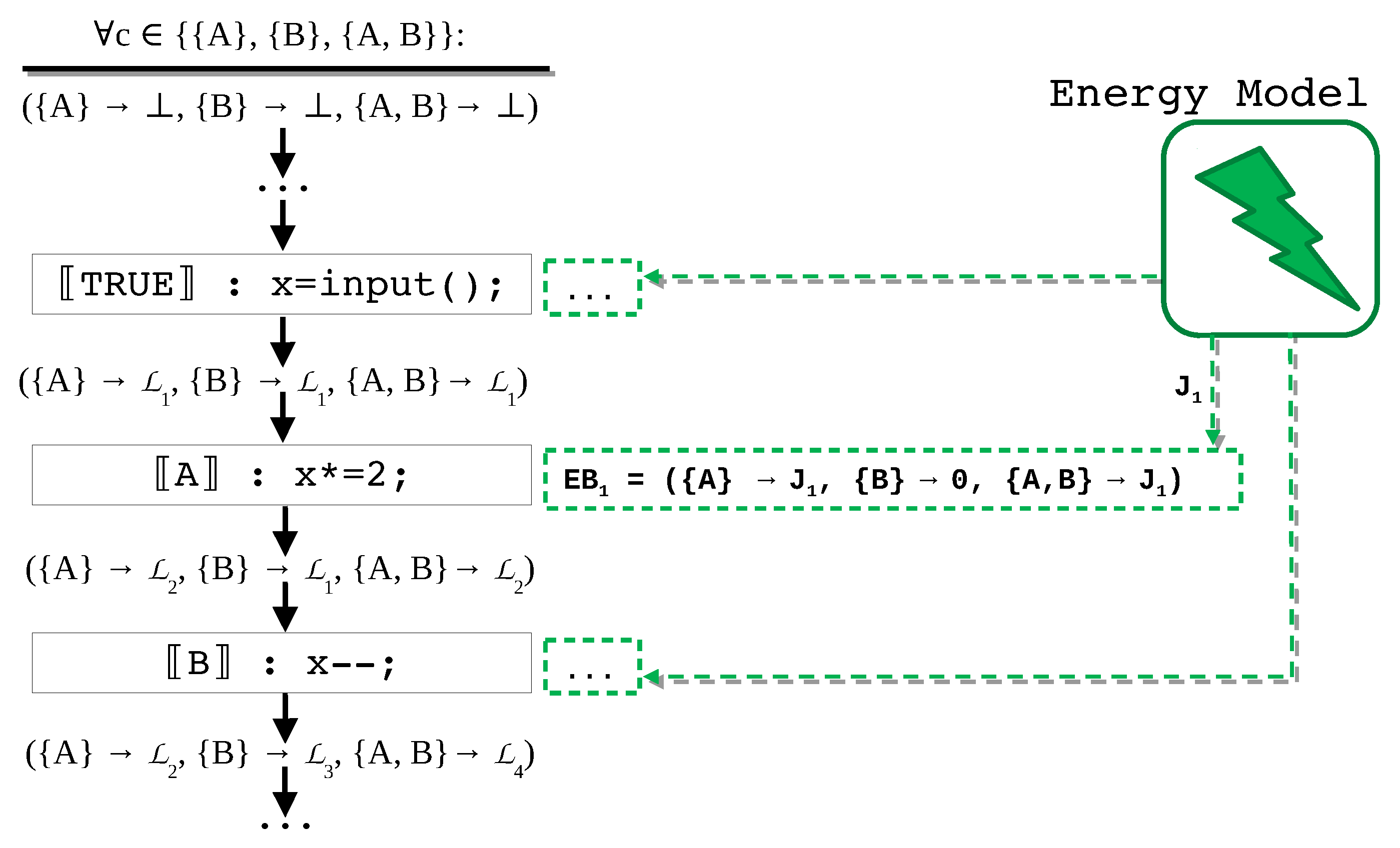