Optimized VLSI Architecture of HEVC Fractional Pixel Interpolators with Approximate Computing


Abstract
1. Introduction
2. Contribution
3. Materials and Methods
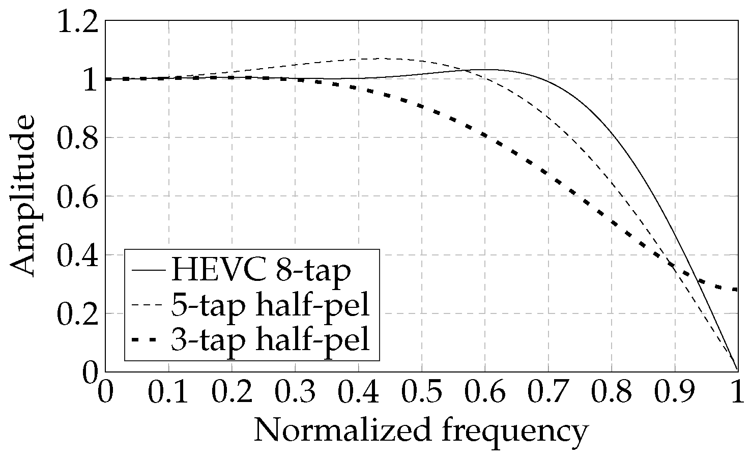
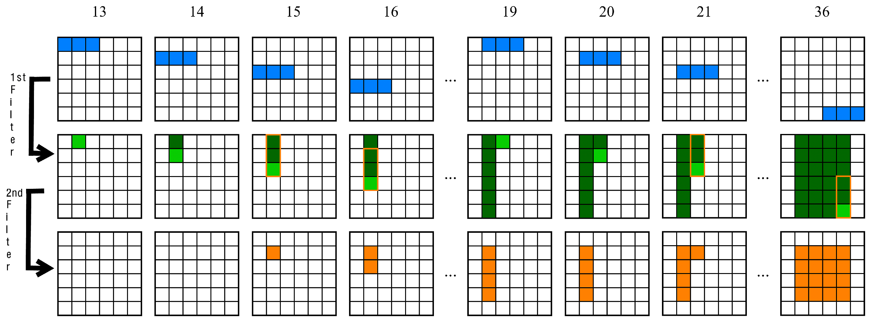
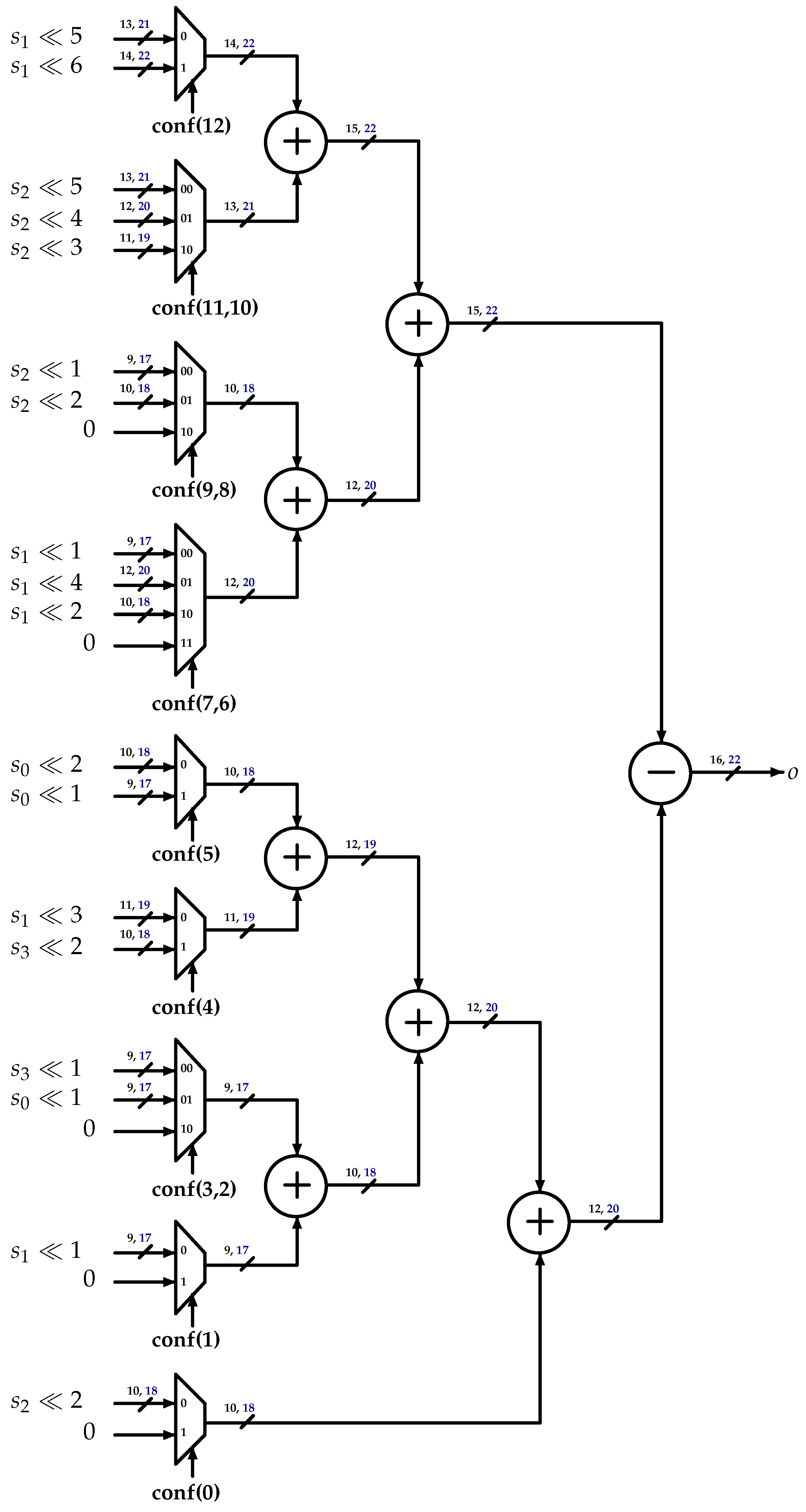
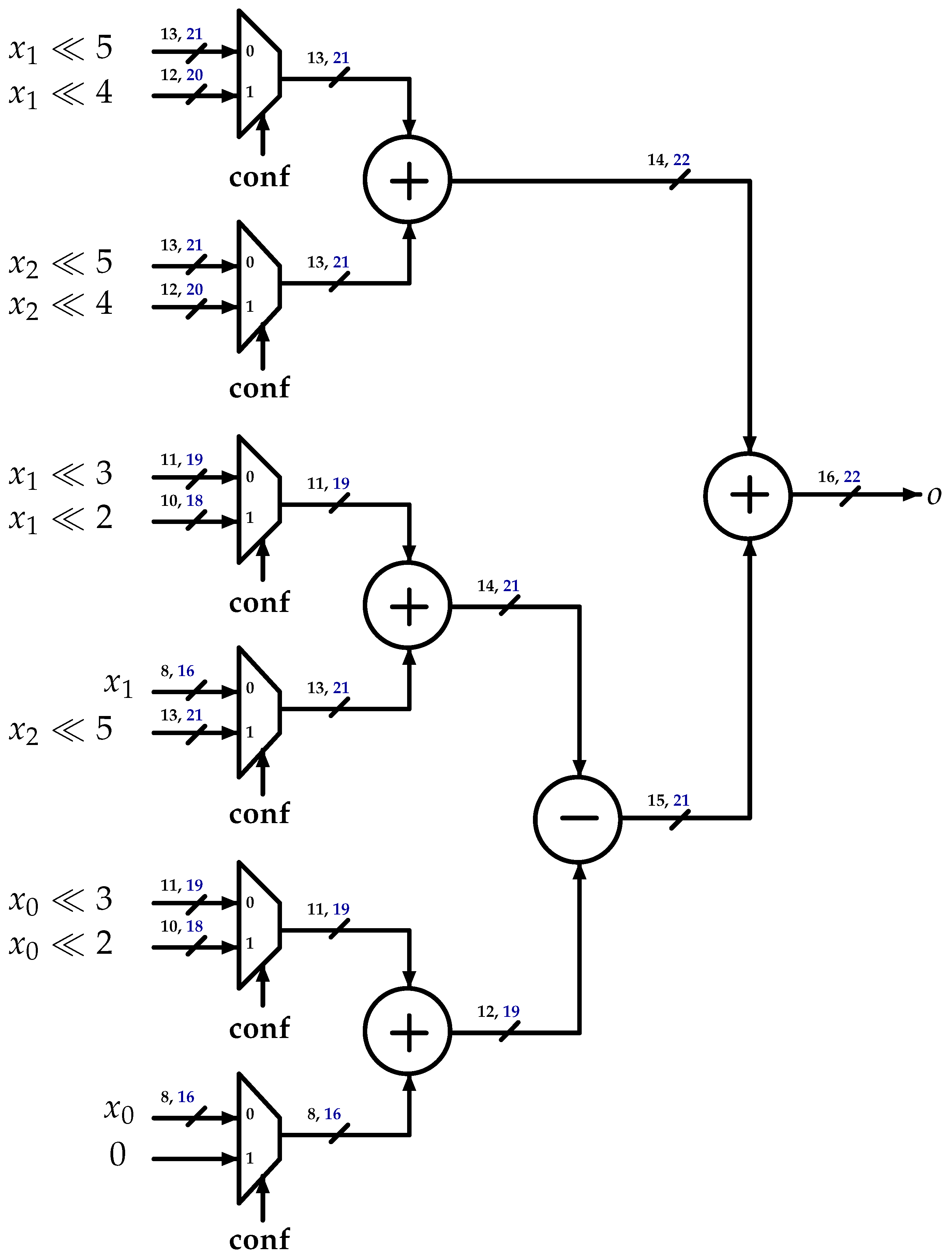
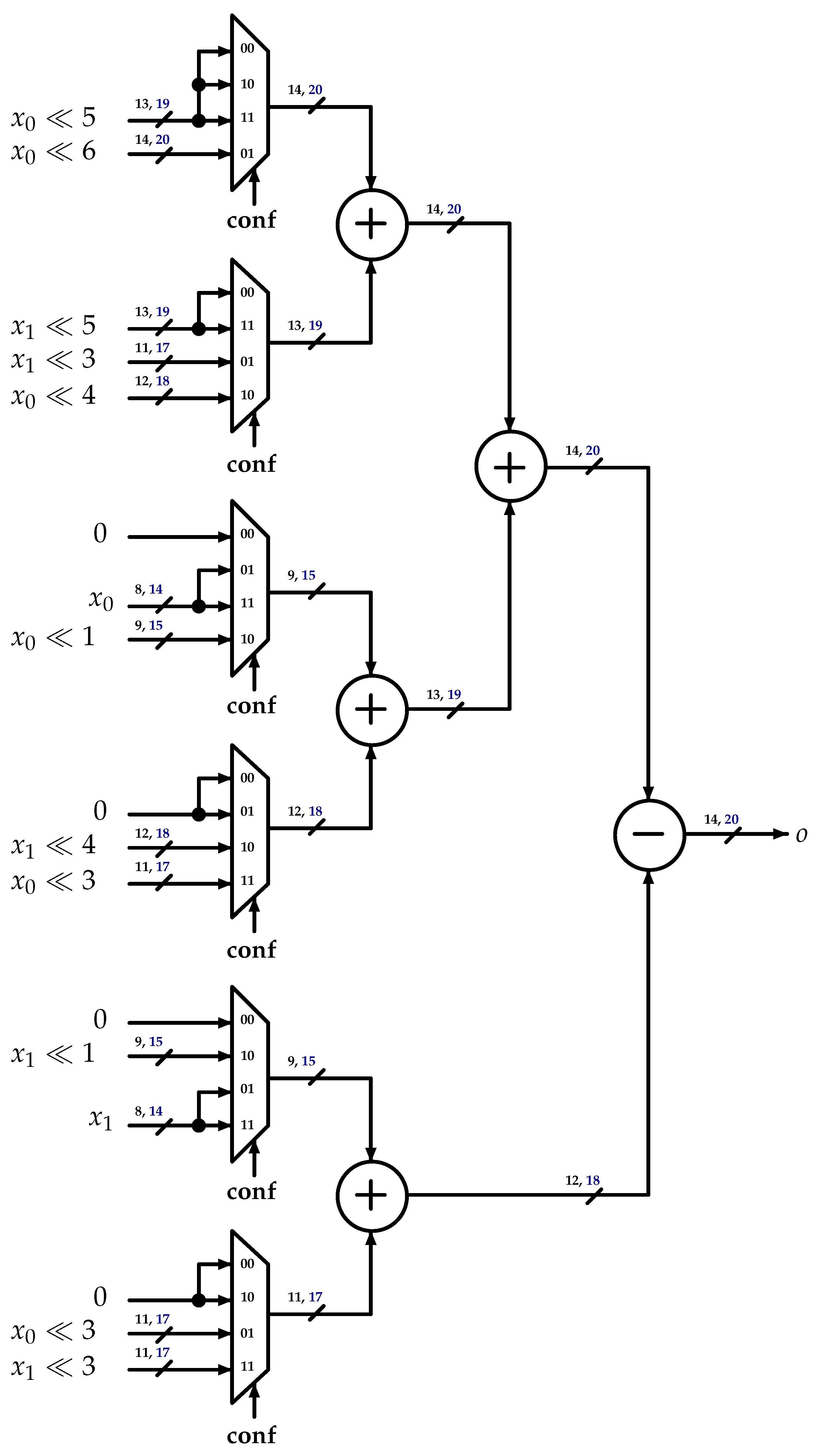
3.1. Interpolation Filters
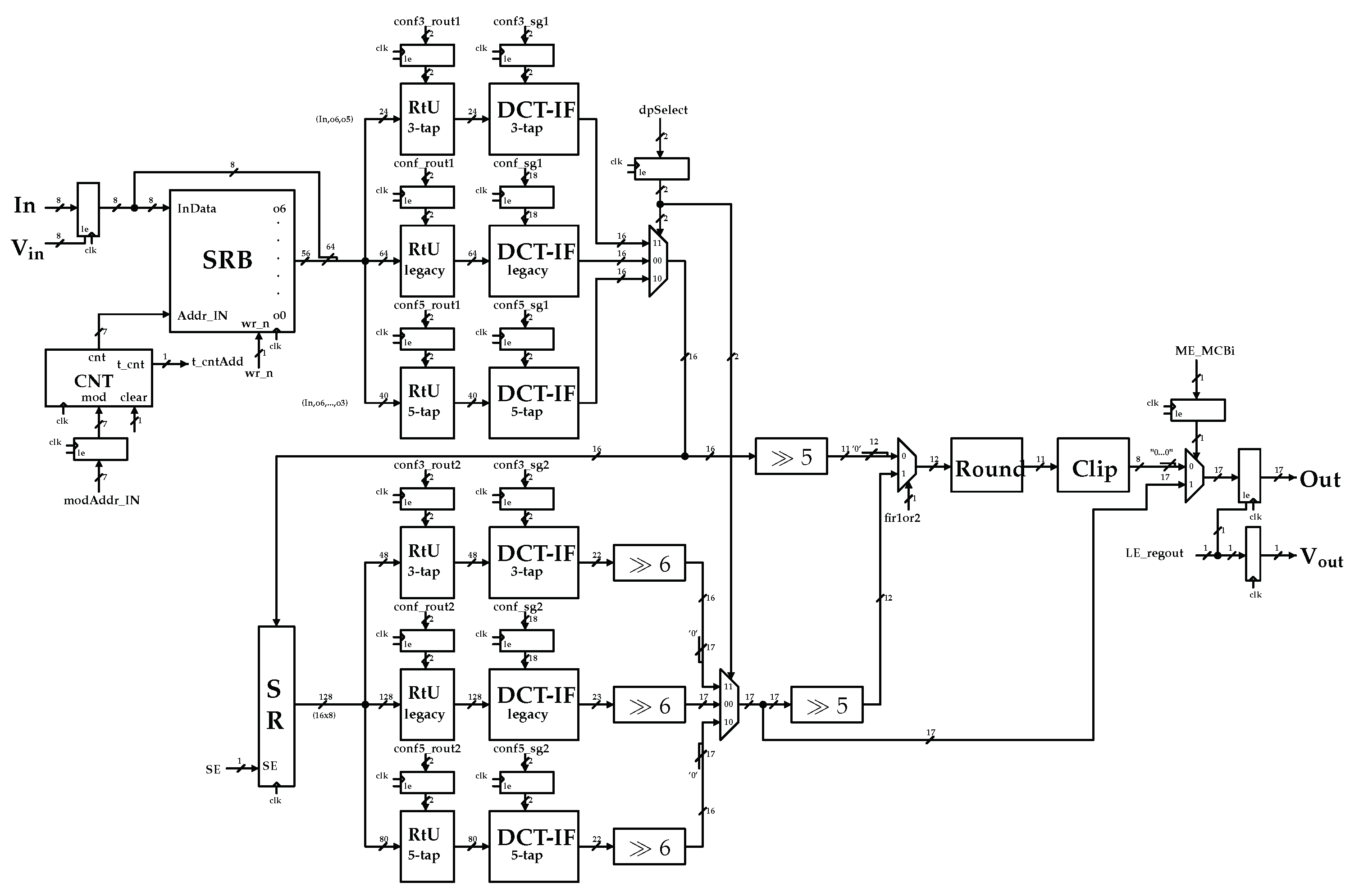
3.2. Proposed Architecture
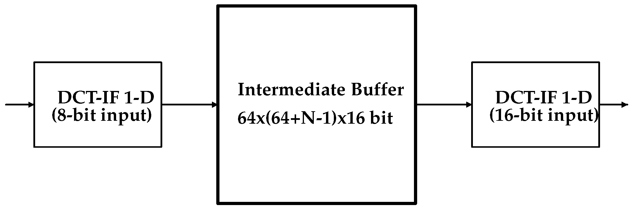
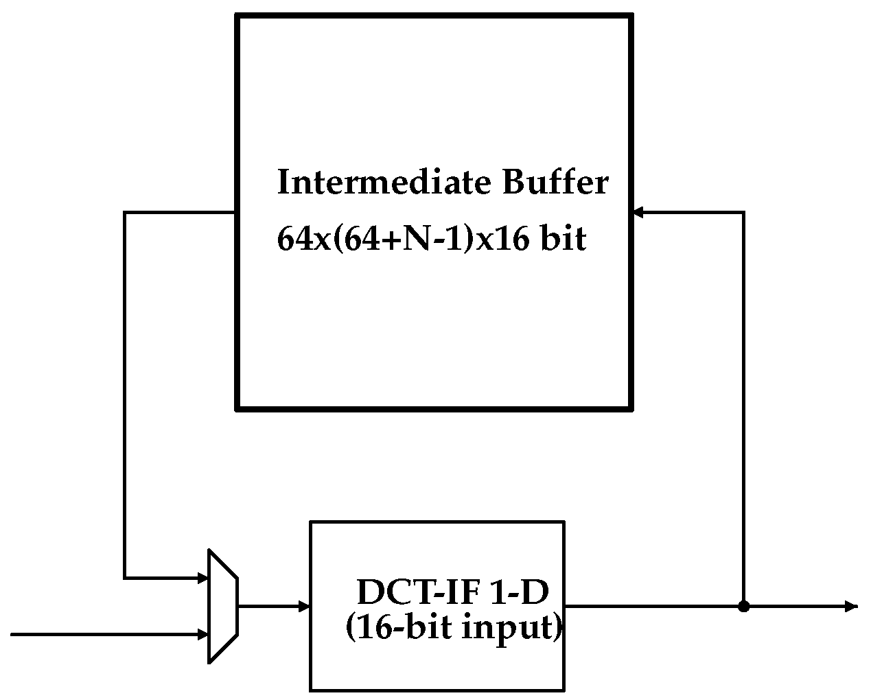
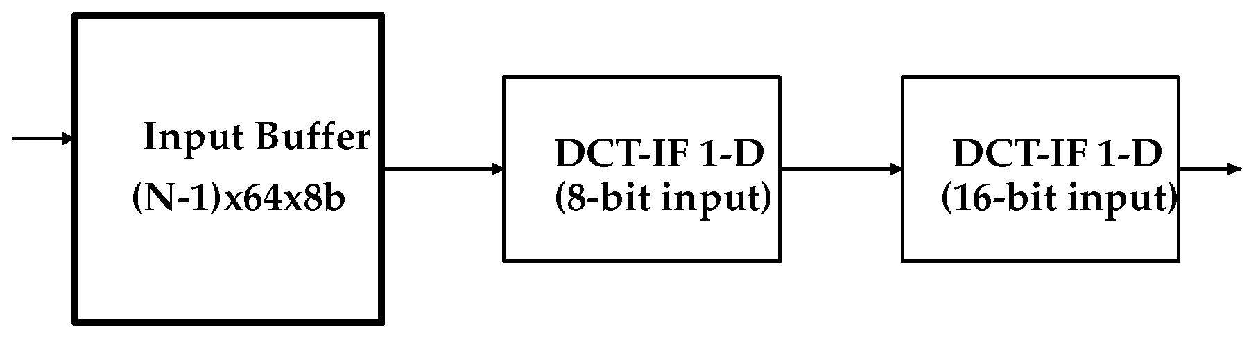
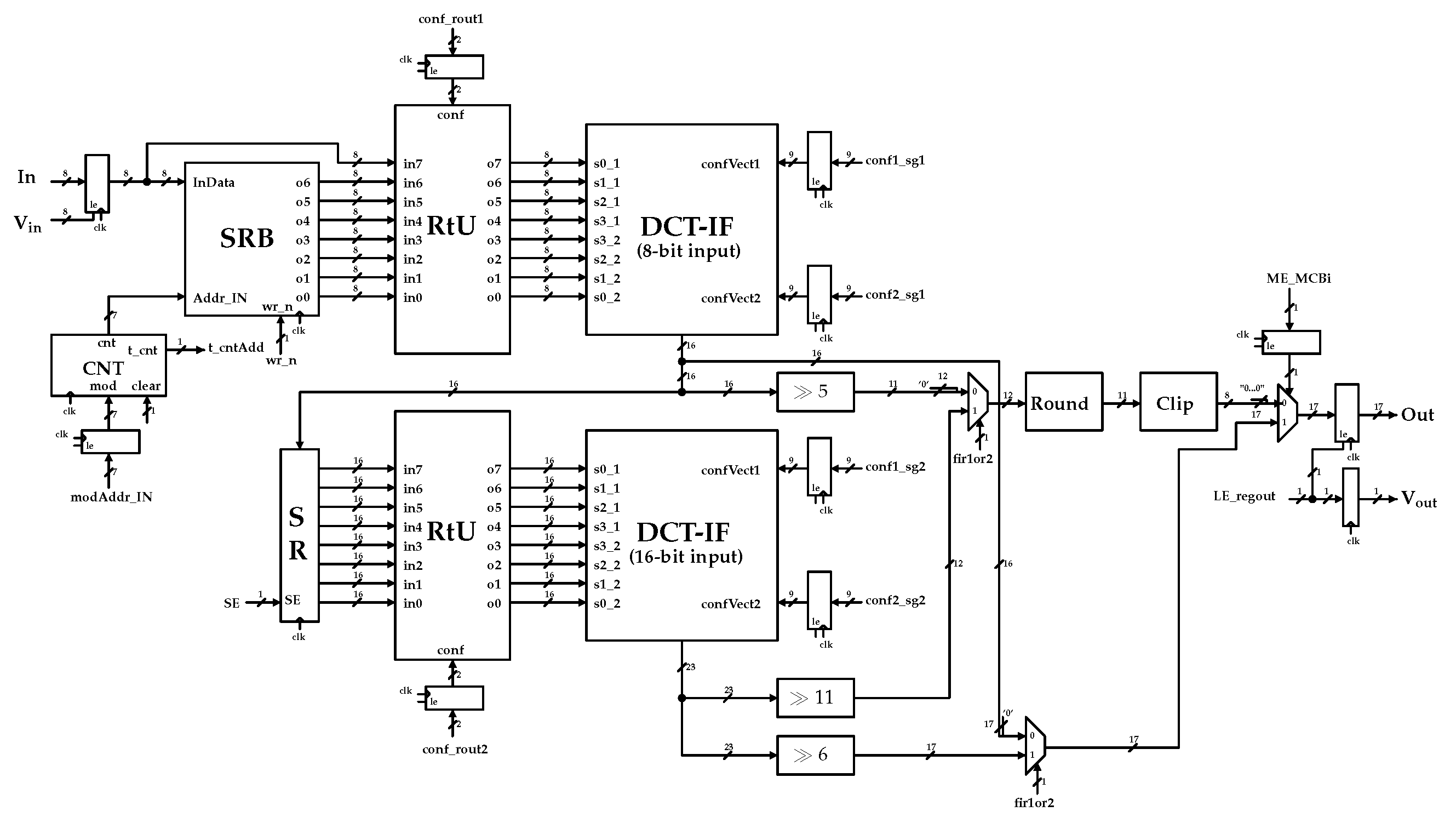
3.3. One-Dimensional DCT-IF Architecture
- Shift Register Bank (SRB): This represents the input buffer. As soon as it receives a pixel row in input it sends it to the RtU and the content of the corresponding Shift Register is shifted.
- Address Counter (CNT): This is a programmable counter that points to a SRB shift register. It fills the lines used to start the filtering process.
- Routing Unit (RtU): This redirects the output of the memory bank toward the inputs of the filter.
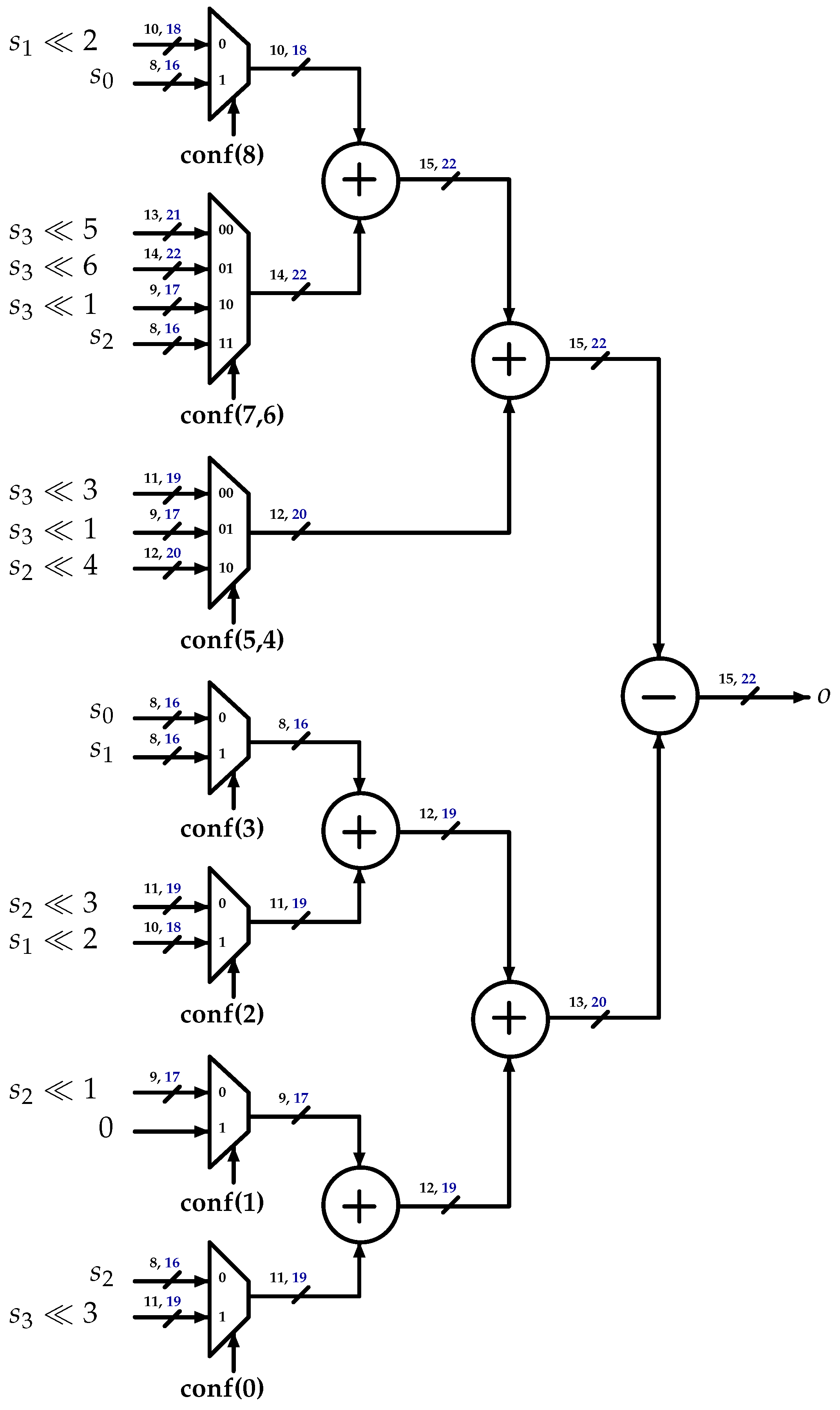
- DCT-IF: This represents the Luma and Chroma legacy multiplier-less architecture described below.
- Rounding Unit (Round): This applies an half-up rounding at the output of the second filter, when required.
- Clipping Unit (Clip): This manages the arithmetic saturation.
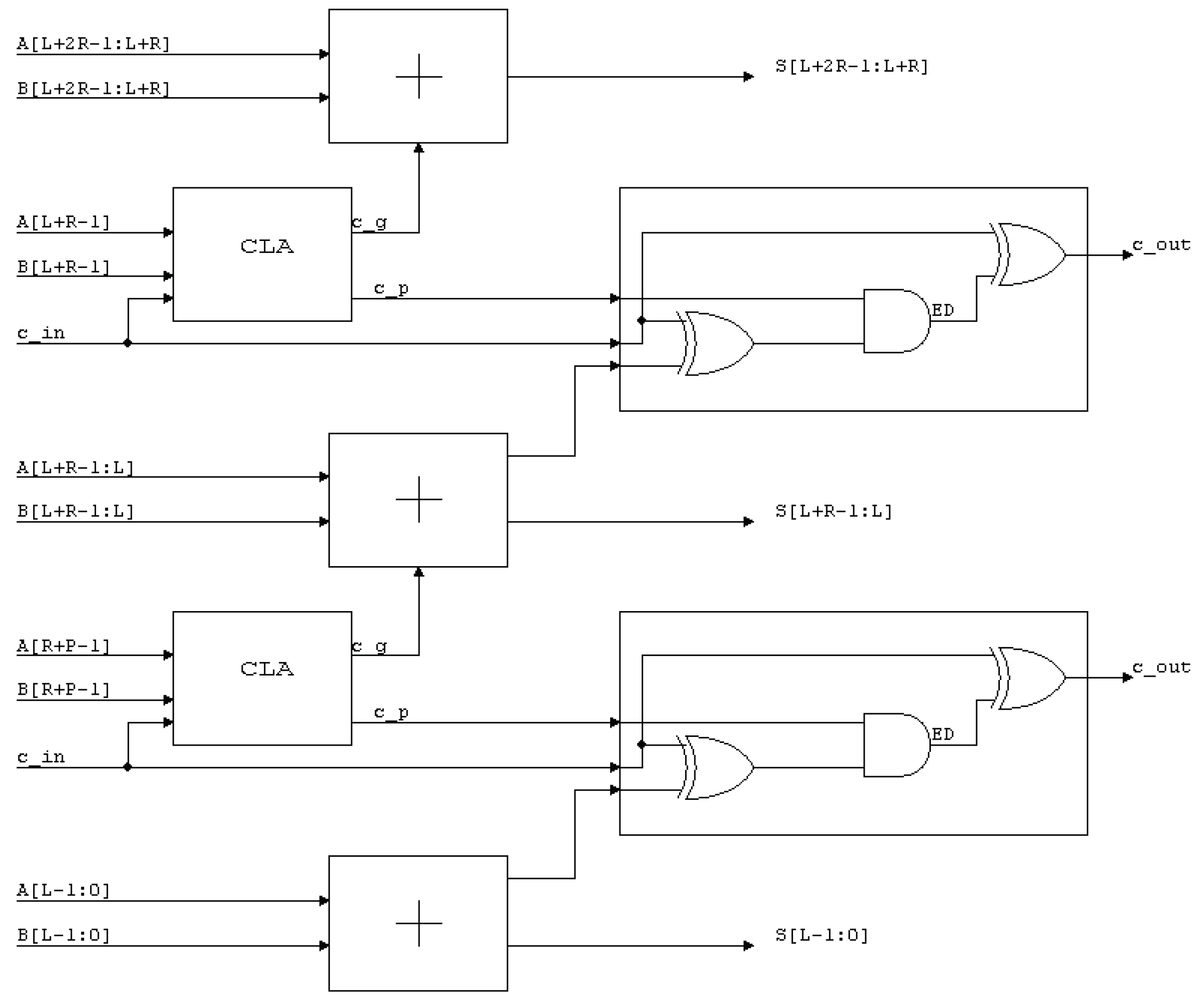
3.4. Optimized Adder Architectures
- Han–Carlson (H.C.): This achieves a good trade-off between complexity, fan-out and perfomance by combining outer Brent–Kung layers and inner Kogge–Stone layers.
- The topology in [16], which uses outer Brent–Kung layers and inner Ladner-Fischer layers. This solution is able to shorten the critical path delay with respect to the tree of prefix operators.
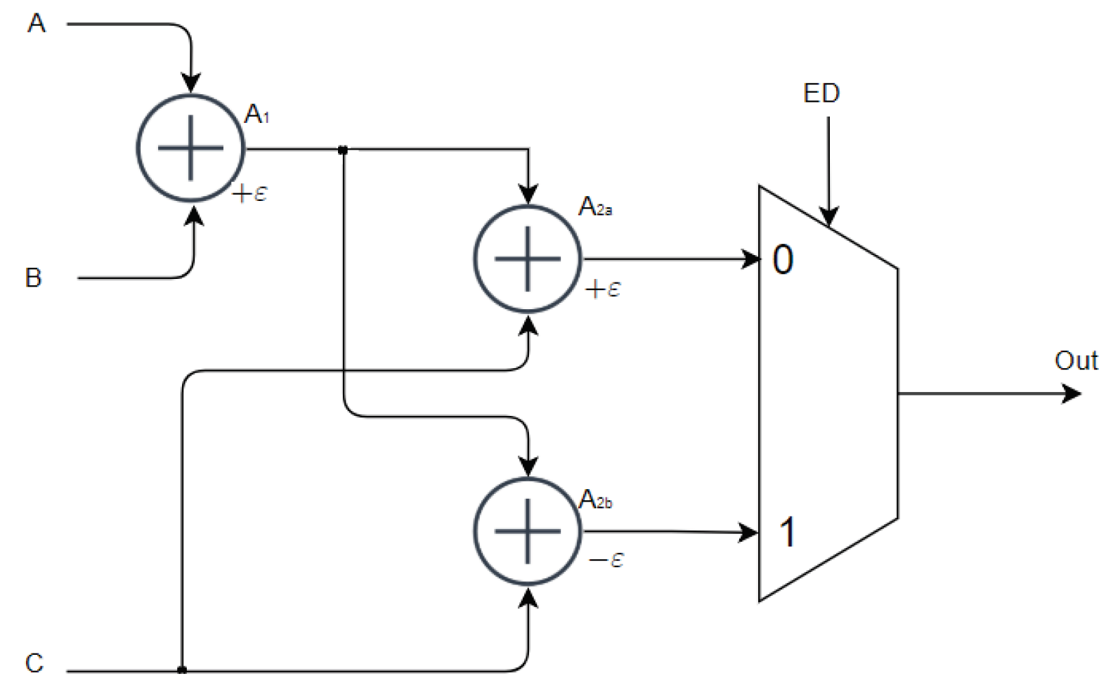
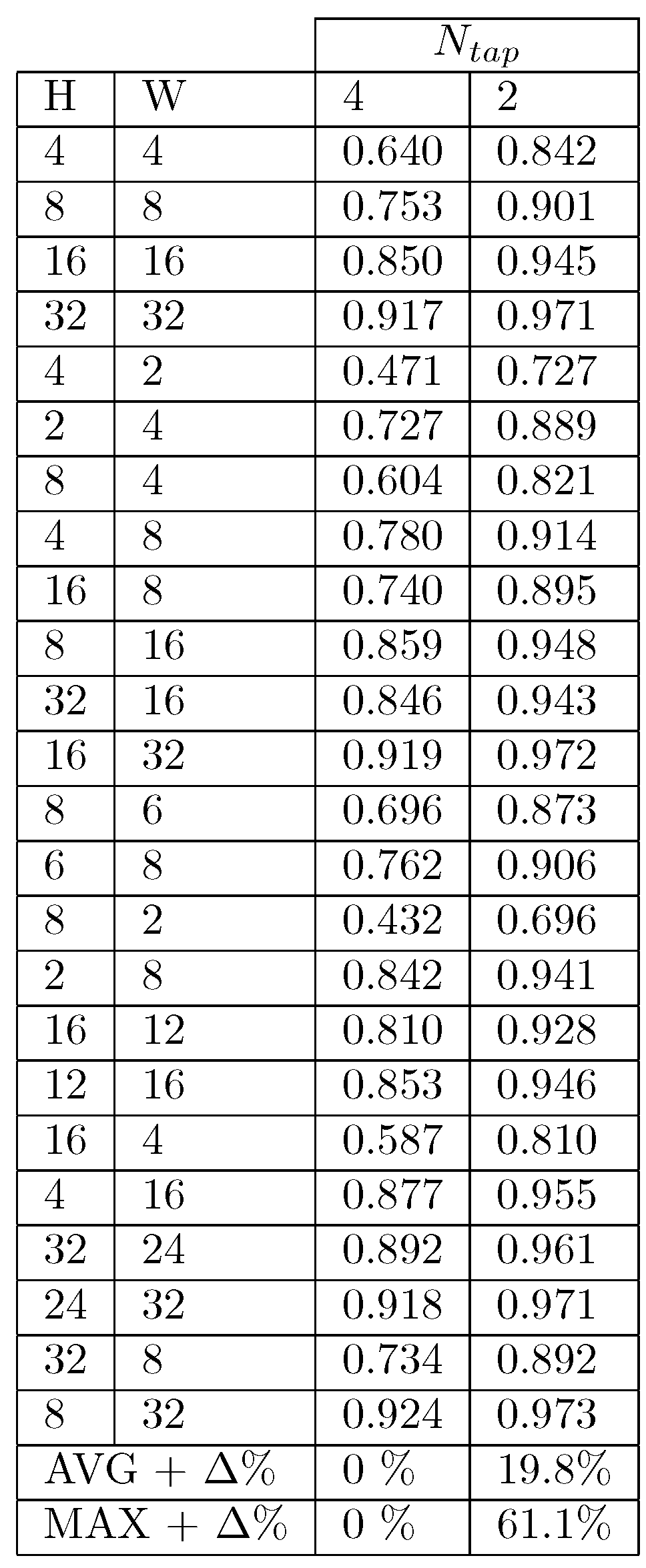
3.5. Generic Accuracy Configurable Adders
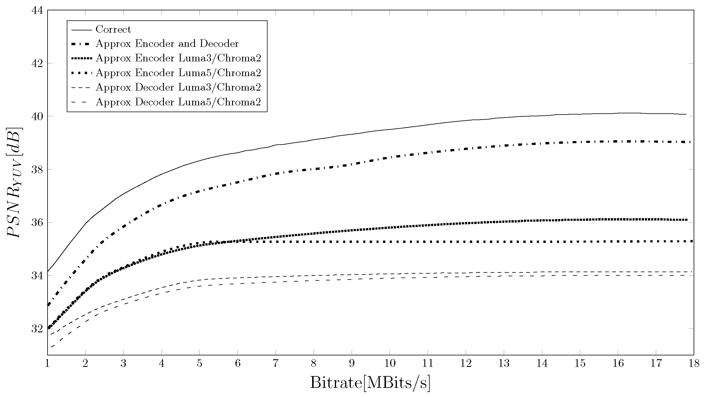
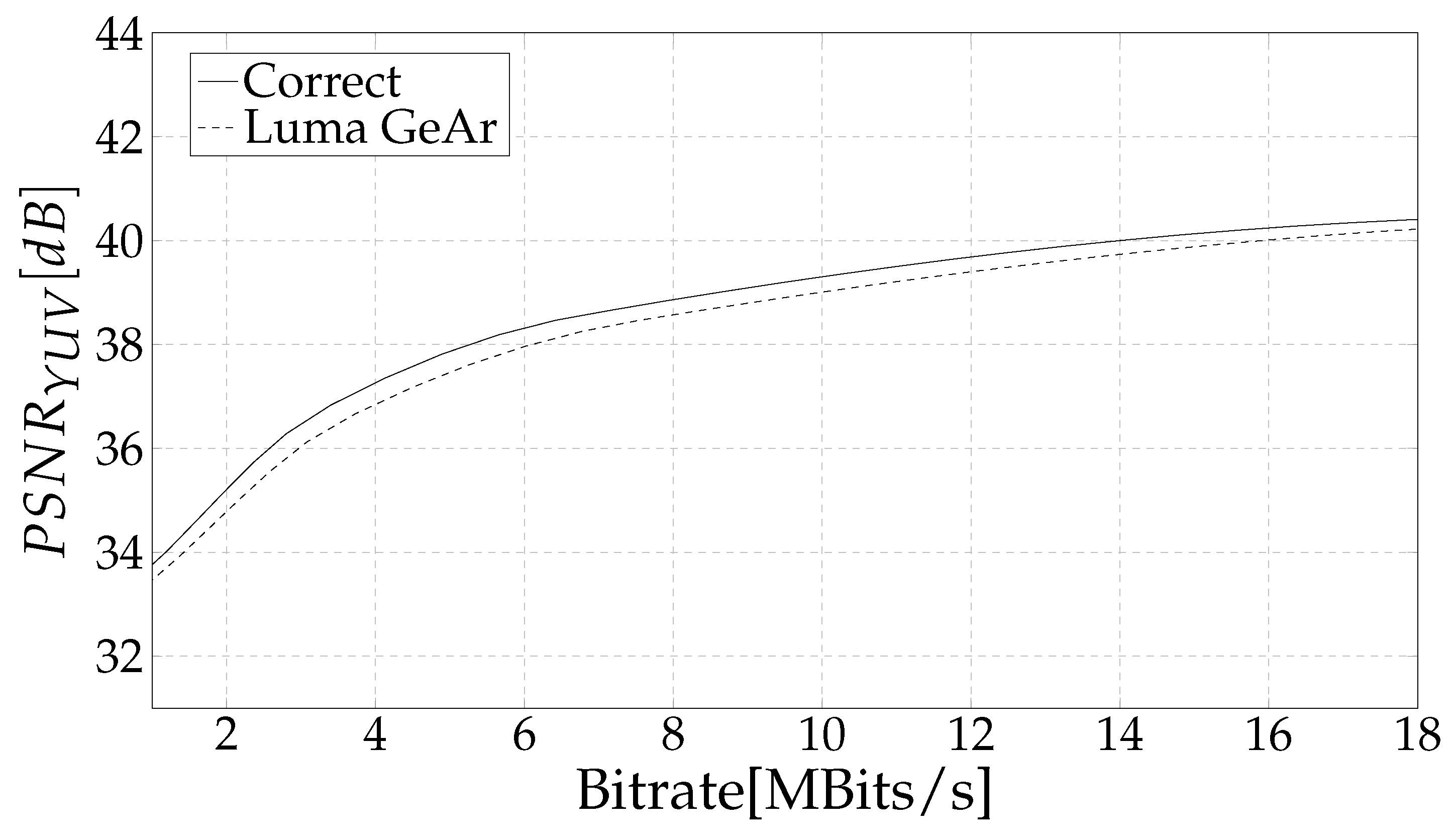
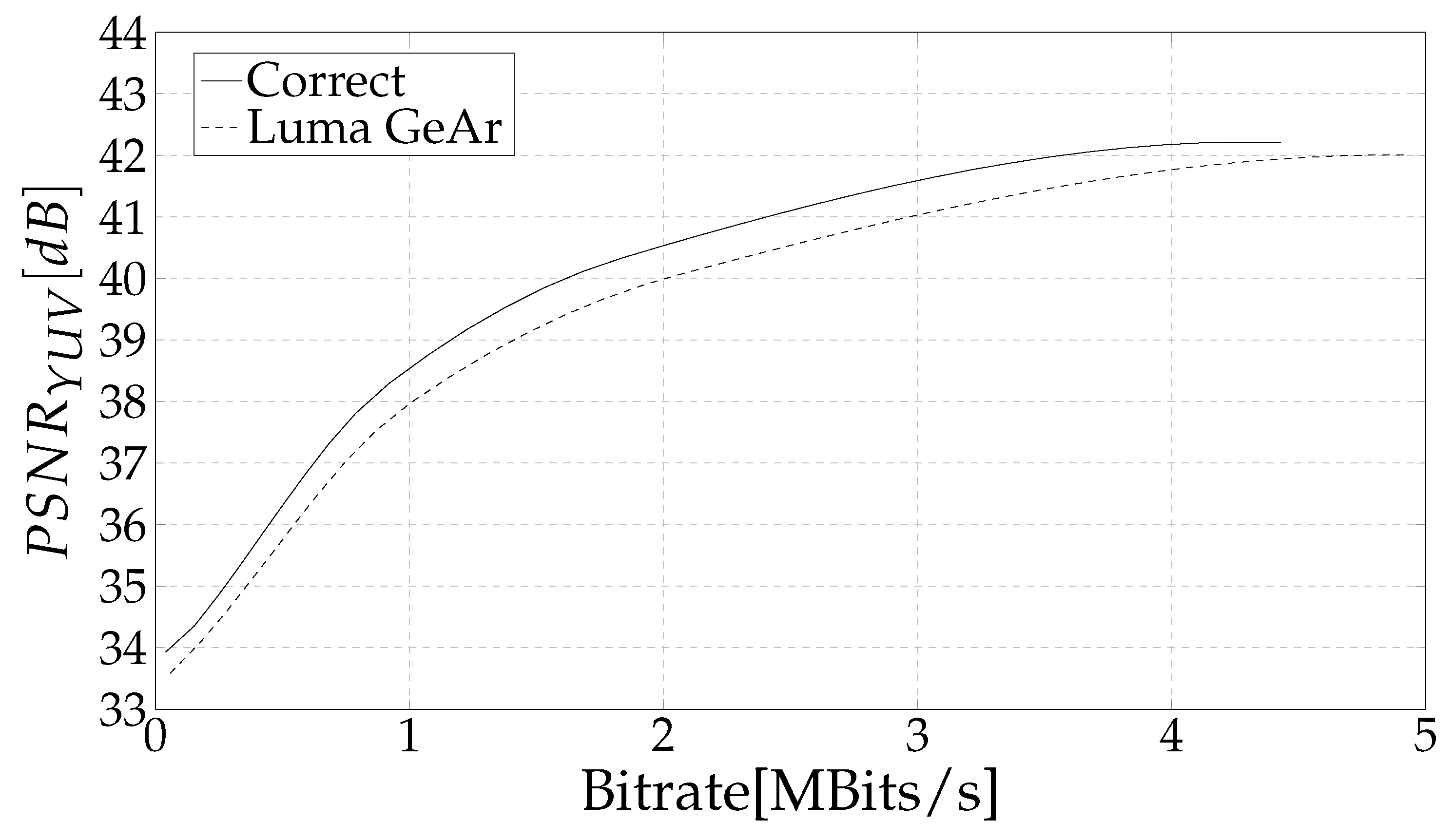
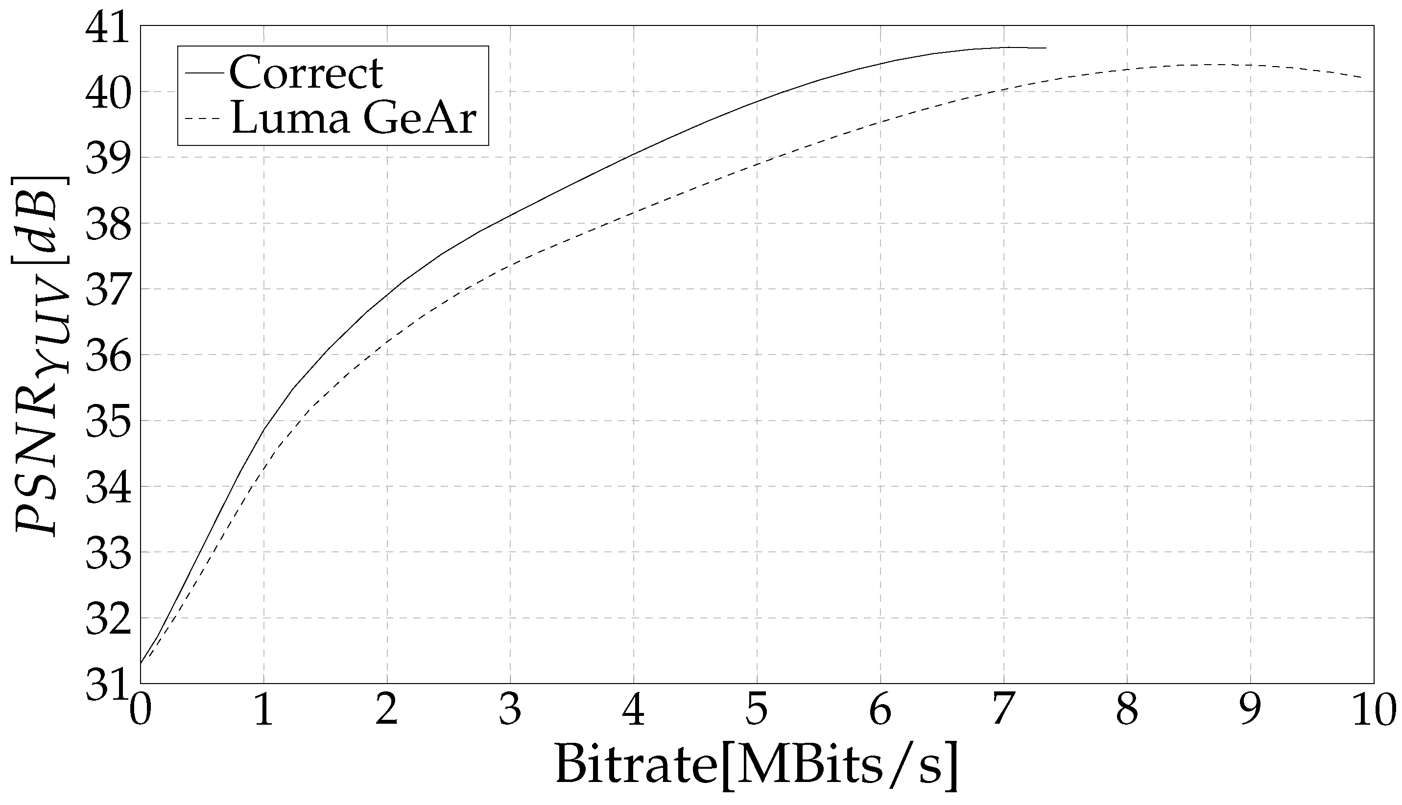
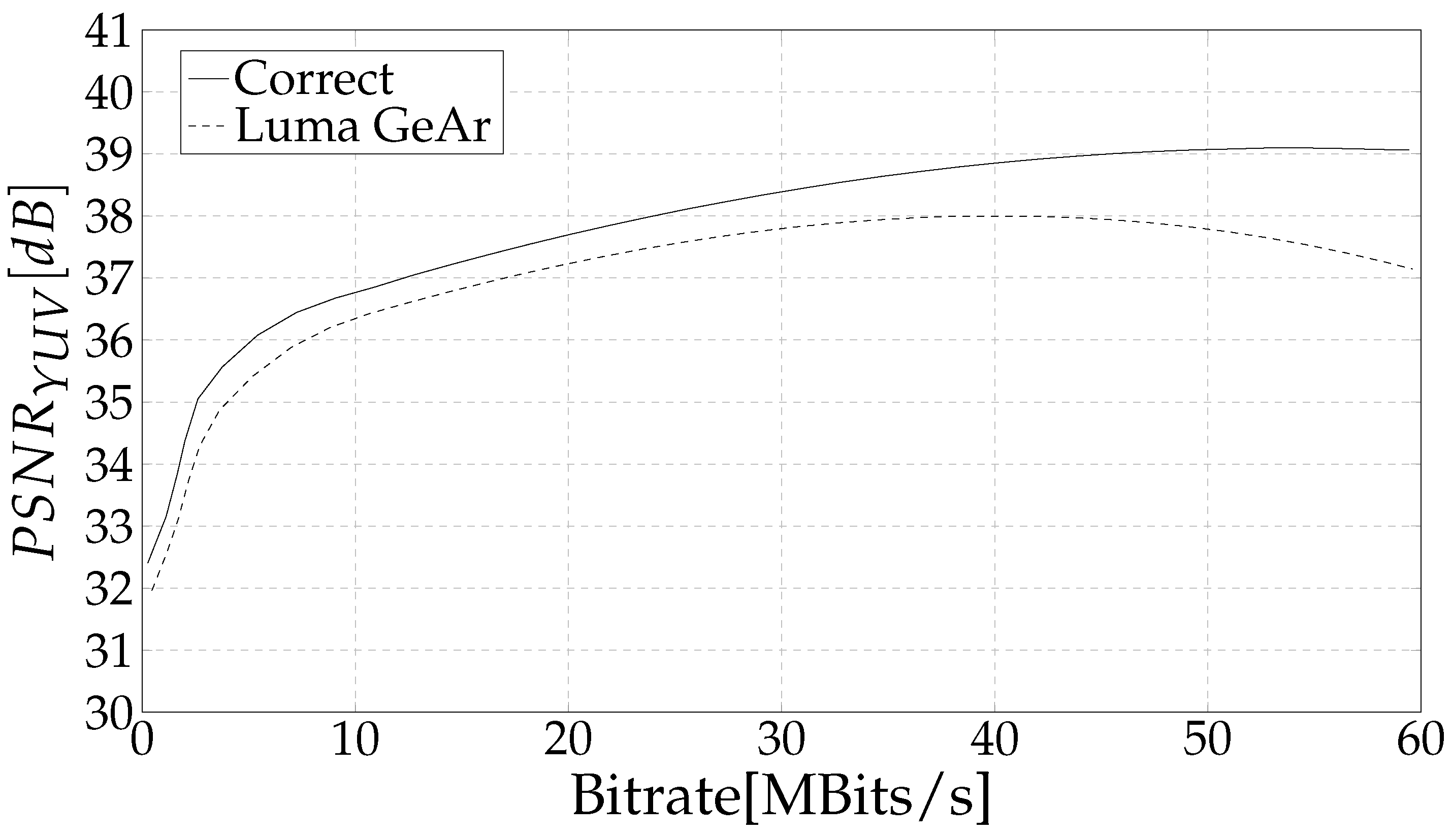
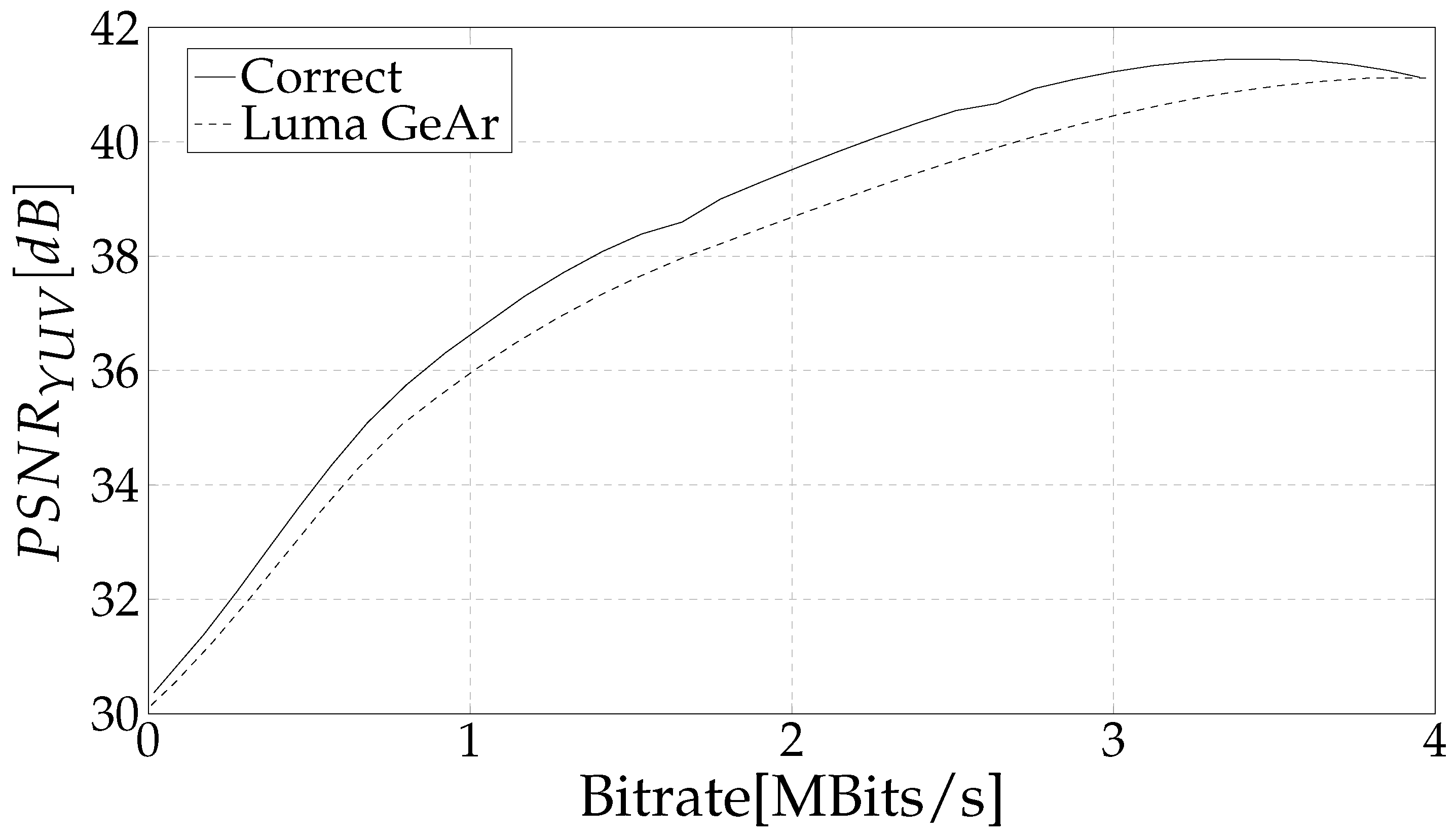
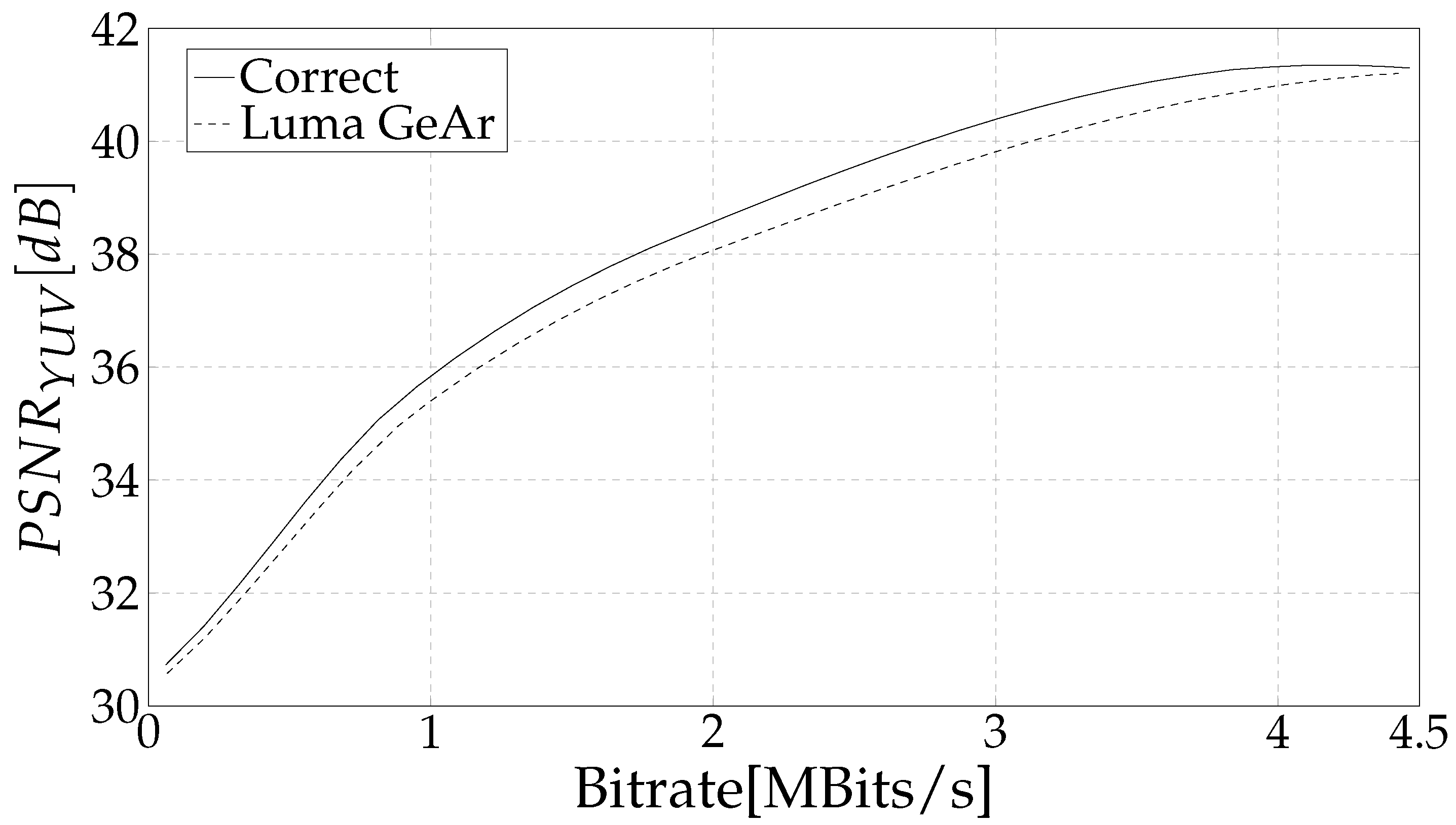
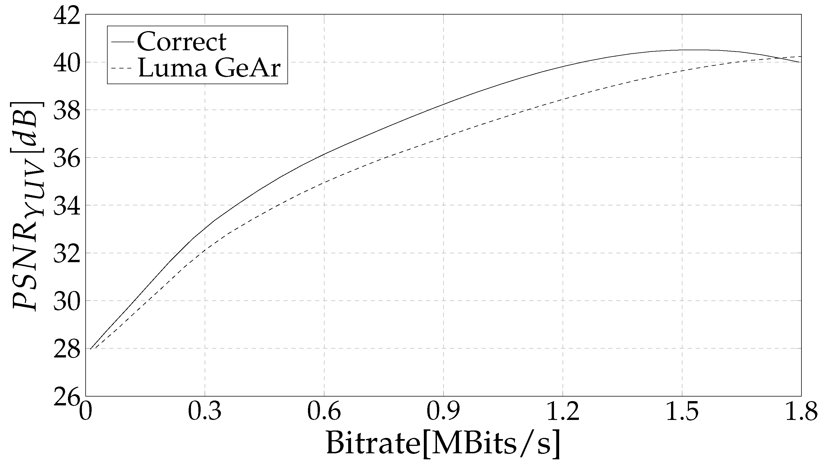
4. Results and Discussion
5. Conclusions
Author Contributions
Funding
Conflicts of Interest
Abbreviations
| HEVC | High Efficient Video Coding |
| AVC | Advanced Video Coding |
| RD | Rate Distorsion |
| RCA | Ripple-Carry Adder |
| PPAs | Parallel Prefix Adders |
| H.C. | Han–Carlson |
| L.F. | Ladner-Fischer |
| EDC | Error Detection and Correction |
| SAM | Standard Approximate Module |
| ED | Error Detection |
| CAM | Complementary Approximate Module |
| GeAr | Generic Accuracy |
| CGeAr | Complementary GeAr |
References
- Ohm, J.R.; Sullivan, G.J.; Schwarz, H.; Tan, T.K.; Wiegand, T. Comparison of the Coding Efficiency of Video Coding Standards-Including High Efficiency Video Coding (HEVC). IEEE Trans. Circuits Syst. Video Technol. 2012, 22, 1669–1684. [Google Scholar] [CrossRef]
- Sayood, K. Introduction to Data Compression, Third Edition (Morgan Kaufmann Series in Multimedia Information and Systems); Morgan Kaufmann Publishers Inc.: San Francisco, CA, USA, 2005; pp. 571–614. [Google Scholar]
- Sullivan, G.J.; Ohm, J.R.; Han, W.J.; Wiegand, T. Overview of the High Efficiency Video Coding (HEVC) Standard. IEEE Trans. Circuits Syst. Video Technol. 2012, 22, 1649–1668. [Google Scholar] [CrossRef]
- Aiyar, M.L.; Kenchappa, R. A high-performance and high-precision sub-pixel motion estimator-interpolator for real-time HDTV(8K) in MPEGH/HEVC coding. In Proceedings of the 2016 International Conference on Emerging Trends in Engineering, Technology and Science (ICETETS), Pudukkottai, India, 24–26 February 2016; pp. 1–8. [Google Scholar]
- Tikekar, M.; Huang, C.; Juvekar, C.; Sze, V.; Chandrakasan, A.P. A 249-Mpixel/s HEVC Video-Decoder Chip for 4K Ultra-HD Applications. IEEE J. Solid-State Circuits 2014, 49, 61–72. [Google Scholar] [CrossRef]
- Da Silva, R.; Siqueira, I.; Grellert, M. Approximate Interpolation Filters for the Fractional Motion Estimation in HEVC Encoders and their VLSI Design. In Proceedings of the 2019 32nd Symposium on Integrated Circuits and Systems Design (SBCCI), Sao Paulo, Brazil, 26–30 August 2019; pp. 1–6. [Google Scholar]
- Guo, Z.; Zhou, D.; Goto, S. An optimized MC interpolation architecture for HEVC. In Proceedings of the 2012 IEEE International Conference on Acoustics, Speech and Signal Processing (ICASSP), Kyoto, Japan, 25–30 March 2012; pp. 1117–1120. [Google Scholar] [CrossRef]
- Afonso, V.; Maich, H.; Agostini, L.; Franco, D. Low cost and high throughput FME interpolation for the HEVC emerging video coding standard. In Proceedings of the IEEE Latin America Symposium on Circuits and Systems, Cusco, Peru, 27 February–1 March 2013; pp. 1–4. [Google Scholar]
- Kalali, E.; Adibelli, Y.; Hamzaoglu, I. A Reconfigurable HEVC sub-pixel interpolation hardware. In Proceedings of the 2013 IEEE Third International Conference on Consumer Electronics, Berlin (ICCE-Berlin), Berlin, Germany, 9–11 September 2013; pp. 125–128. [Google Scholar] [CrossRef]
- Diniz, C.M.; Shafique, M.; Bampi, S.; Henkel, J. A Reconfigurable Hardware Architecture for Fractional Pixel Interpolation in High Efficiency Video Coding. IEEE Trans. Comput. Aided Des. Integr. Circuits Syst. 2015, 34, 238–251. [Google Scholar] [CrossRef]
- Diefy, A.; Shalaby, A.; Sayed, M.S. Low cost Luma interpolation filter for motion compensation in HEVC. In Proceedings of the 2016 IEEE 59th International Midwest Symposium on Circuits and Systems (MWSCAS), Abu Dhabi, UAE, 16–19 October 2016; pp. 1–4. [Google Scholar] [CrossRef]
- Ghani, A.; Kalali, E.; Hamzaoglu, I. FPGA implementations of HEVC sub-pixel interpolation using high-level synthesis. In Proceedings of the IEEE International Conference on Design and Technology of Integrated Systems in Nanoscale Era, Istanbul, Turkey, 12–14 April 2016; pp. 1–4. [Google Scholar]
- Sau, C.; Palumbo, F.; Pelcat, M.; Heulot, J.; Nogues, E.; Menard, D.; Meloni, P.; Raffo, L. Challenging the Best HEVC Fractional Pixel FPGA Interpolators With Reconfigurable and Multifrequency Approximate Computing. IEEE Embed. Syst. Lett. 2017, 9, 65–68. [Google Scholar] [CrossRef]
- Bossen, F.; Bross, B.; Suhring, K.; Flynn, D. HEVC Complexity and Implementation Analysis. IEEE Trans. Circuits Syst. Video Technol. 2012, 22, 1685–1696. [Google Scholar] [CrossRef]
- Nogues, E.; Menard, D.; Pelcat, M. Algorithmic-level Approximate Computing Applied to Energy Efficient HEVC Decoding. IEEE Trans. Emerg. Top. Comput. 2016, 1–12. [Google Scholar] [CrossRef]
- Esposito, D.; Caro, D.D.; Strollo, A.G.M. Variable Latency Speculative Parallel Prefix Adders for Unsigned and Signed Operands. IEEE Trans. Circuits Syst. 2016, 63, 1200–1209. [Google Scholar] [CrossRef]
- Mazahir, S.; Hasan, O.; Shafique, M. Adaptive Approximate Computing in Arithmetic Datapaths. IEEE Des. Test 2017, 35, 65–74. [Google Scholar]
- ITU-T Video Coding Experts Group; ISO/IEC Moving Picture Experts Group. HM16.15. Available online: https://hevc.hhi.fraunhofer.de/svn/svn_HEVCSoftware/tags/HM-16.15/ (accessed on 20 June 2020).
- Ugur, K.; Alshin, A.; Alshina, E.; Bossen, F.; Han, W.J.; Park, J.H.; Lainema, J. Motion Compensated Prediction and Interpolation Filter Design in H.265/HEVC. IEEE J. Sel. Top. Signal Process. 2013, 7, 946–956. [Google Scholar] [CrossRef]
- Bossen, F. Common test conditions and software reference configurations. In Proceedings of the Joint Collaborative Team on Video Coding (JCT-VC) of ITU-T SG 16 Wp 3 and ISO/IEC JTC 1/SC 29/WG 11, 12th Meeting, Geneva, Switzerland, 14–23 January 2013. [Google Scholar]
- Macedo, M.; Soares, L.; Silveira, B.; Diniz, C.M.; da Costa, E.A.C. Exploring the Use of Parallel Prefix Adder Topologies into Approximate Adder Circuits. In Proceedings of the IEEE Transactions on Circuits and Systems, Batumi, Georgia, 5–8 December 2017; pp. 298–301. [Google Scholar]
- Shafique, M.; Ahmad, W.; Hafiz, R.; Henkel, J. A low latency generic accuracy configurable adder. In Proceedings of the 52nd Annual Design Automation Conference, San Francisco, CA, USA, 8–12 June 2015; p. 86. [Google Scholar]
- UMC. 65 Nanometer. Available online: http://www.umc.com/english/pdf/UMC%2065nm.pdf (accessed on 1 September 2018).Now Available online: https://www.umc.com/en/Product/process_technologies/Detail/55_65_90nm (accessed on 10 June 2020).


| Legacy | ||
| 7 | ||
| 5 | ||
| 3 | ||
| 1 | 64 | 64 |
| Legacy | ||||
| 64 | 64 | 64 | 64 |
| Shift—Coeff | 1 | 2 | 4 | 5 | 6 | 7 | 9 | 14 | 20 | 23 | 32 | 40 | 41 | 48 | 50 | 54 | 57 |
|---|---|---|---|---|---|---|---|---|---|---|---|---|---|---|---|---|---|
| + | + | − | + | − | + | + | |||||||||||
| + | + | − | + | + | |||||||||||||
| + | + | + | + | + | |||||||||||||
| + | + | − | + | + | − | ||||||||||||
| + | + | + | + | + | |||||||||||||
| + | + | + | + | + | + | + | |||||||||||
| + |
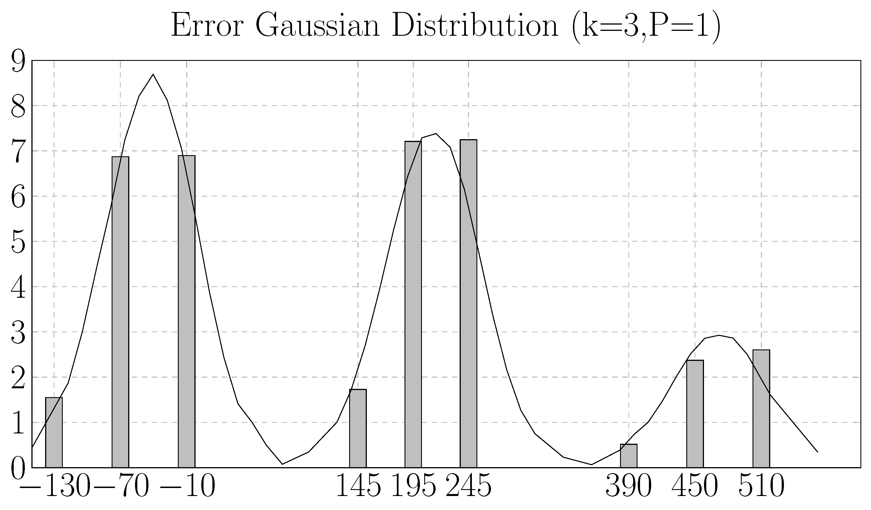
| Gaussian 1 | Gaussian 2 | Gaussian 3 | |
|---|---|---|---|
| –41.09 | 214.23 | 472.73 | |
| 41.98 | 42.51 | 41.63 |
| P [mW] | [MHz] | Technology | A [m] | [] | ||
|---|---|---|---|---|---|---|
| Luma Legacy [13] | 8 | 11 | 213 | Artix-7 28 nm FPGA | - | - |
| Luma Approximated [13] | 8 | 12 | 200 | Artix-7 28 nm FPGA | - | - |
| 7 | 11 | 200 | Artix-7 28 nm FPGA | - | - | |
| 5 | 10 | 200 | Artix-7 28 nm FPGA | - | - | |
| 3 | 10 | 200 | Artix-7 28 nm FPGA | - | - | |
| Luma Legacy [6] | 8 | - | 76.49 | Intel 60 nm FPGA | - | - |
| Luma Legacy [11] | 8 | - | 384 | 65 nm | - | - |
| Luma Legacy | 8 | 9.95 (+0%) | 435 | 65 nm | 60.28 | |
| Luma Legacy GeAr | 8 | 10.589 (+6.42%) | 450 | 65 nm | 65.04 | |
| Luma 5-tap | 5 | 9.062 (–8.92%) | 438 | 65 nm | 66.89 | |
| Luma 5-tap H.C. | 5 | 9.131 (–8.23%) | 427 | 65 nm | 65.31 | |
| Luma 3-tap | 3 | 7.384 (–25.8%) | 438 | 65 nm | 66.89 | |
| Luma 3-tap H.C | 3 | 7.057 (–29.1%) | 427 | 65 nm | 65.31 |
| 8 | 5 | 3 | |
|---|---|---|---|
| P [mW] | [MHz] | Technology | A [m] | [] | ||
|---|---|---|---|---|---|---|
| Chroma Legacy [13] | 4 | 9 | 217 | Artix-7 28 nm FPGA | - | - |
| Chroma | 4 | 9 | 200 | Artix-7 28 nm FPGA | - | - |
| Approximated | 3 | 8 | 200 | Artix-7 28 nm FPGA | - | - |
| [13] | 2 | 6 | 200 | Artix-7 28 nm FPGA | - | - |
| Chroma Legacy | 4 | 2.966 (+0%) | 501 | 65 nm | 21.99 | |
| Chroma Legacy | 4 | 3.013(+1.58%) | 479 | 65 nm | 15.75 | |
| Adder [16] | ||||||
| Chroma 2-tap | 2 | 2.157 (–27.3%) | - | 65 nm | - | - |
| 4 | 2 | |
|---|---|---|
© 2020 by the authors. Licensee MDPI, Basel, Switzerland. This article is an open access article distributed under the terms and conditions of the Creative Commons Attribution (CC BY) license (http://creativecommons.org/licenses/by/4.0/).
Share and Cite
Preatto, S.; Giannini, A.; Valente, L.; Masera, G.; Martina, M. Optimized VLSI Architecture of HEVC Fractional Pixel Interpolators with Approximate Computing. J. Low Power Electron. Appl. 2020, 10, 24. https://doi.org/10.3390/jlpea10030024
Preatto S, Giannini A, Valente L, Masera G, Martina M. Optimized VLSI Architecture of HEVC Fractional Pixel Interpolators with Approximate Computing. Journal of Low Power Electronics and Applications. 2020; 10(3):24. https://doi.org/10.3390/jlpea10030024
Chicago/Turabian StylePreatto, Stefania, Andrea Giannini, Luca Valente, Guido Masera, and Maurizio Martina. 2020. "Optimized VLSI Architecture of HEVC Fractional Pixel Interpolators with Approximate Computing" Journal of Low Power Electronics and Applications 10, no. 3: 24. https://doi.org/10.3390/jlpea10030024
APA StylePreatto, S., Giannini, A., Valente, L., Masera, G., & Martina, M. (2020). Optimized VLSI Architecture of HEVC Fractional Pixel Interpolators with Approximate Computing. Journal of Low Power Electronics and Applications, 10(3), 24. https://doi.org/10.3390/jlpea10030024