Low-Power Embedded System for Gait Classification Using Neural Networks

 ,
,  ,
,  and
and 
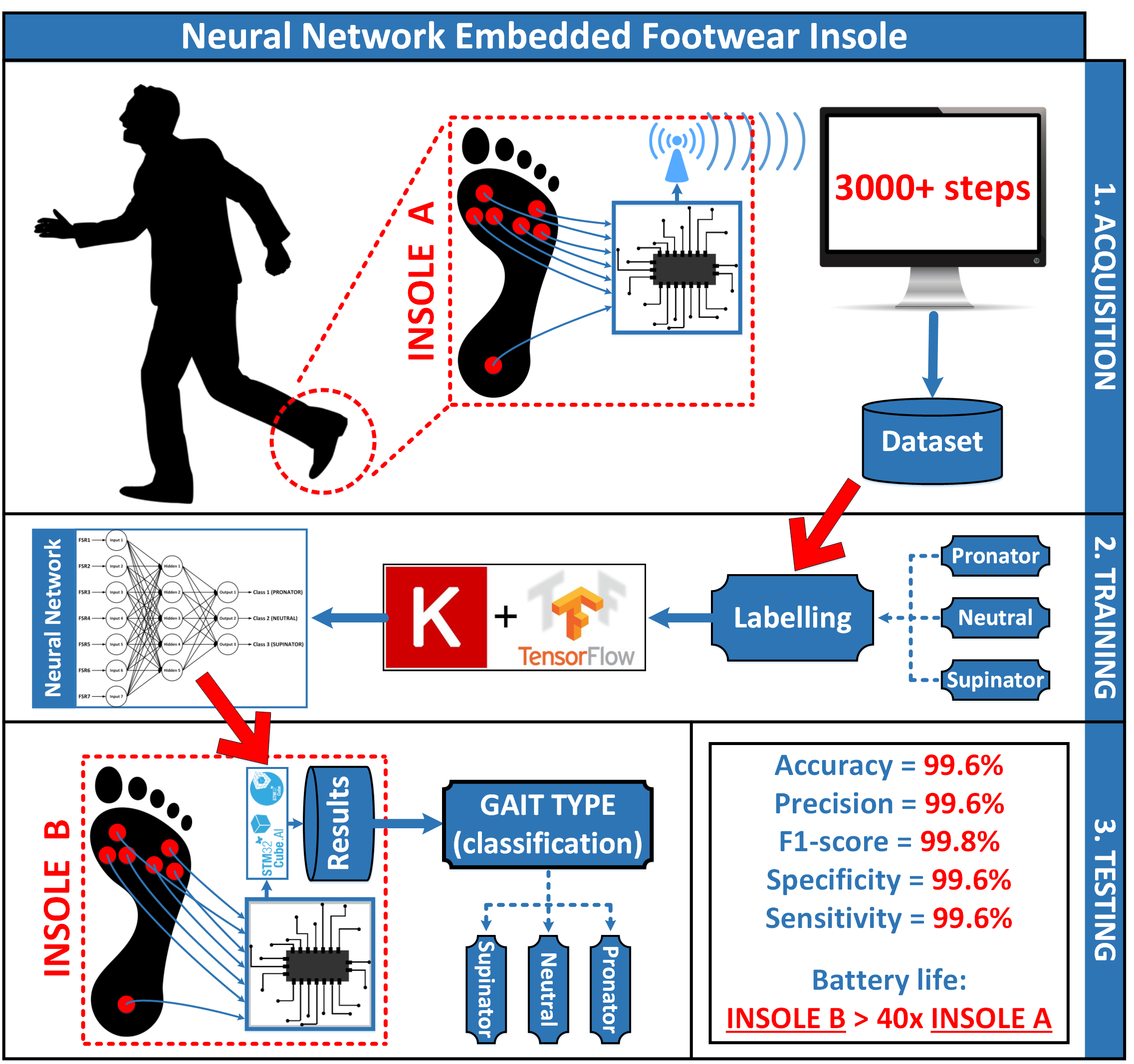
Abstract

1. Introduction
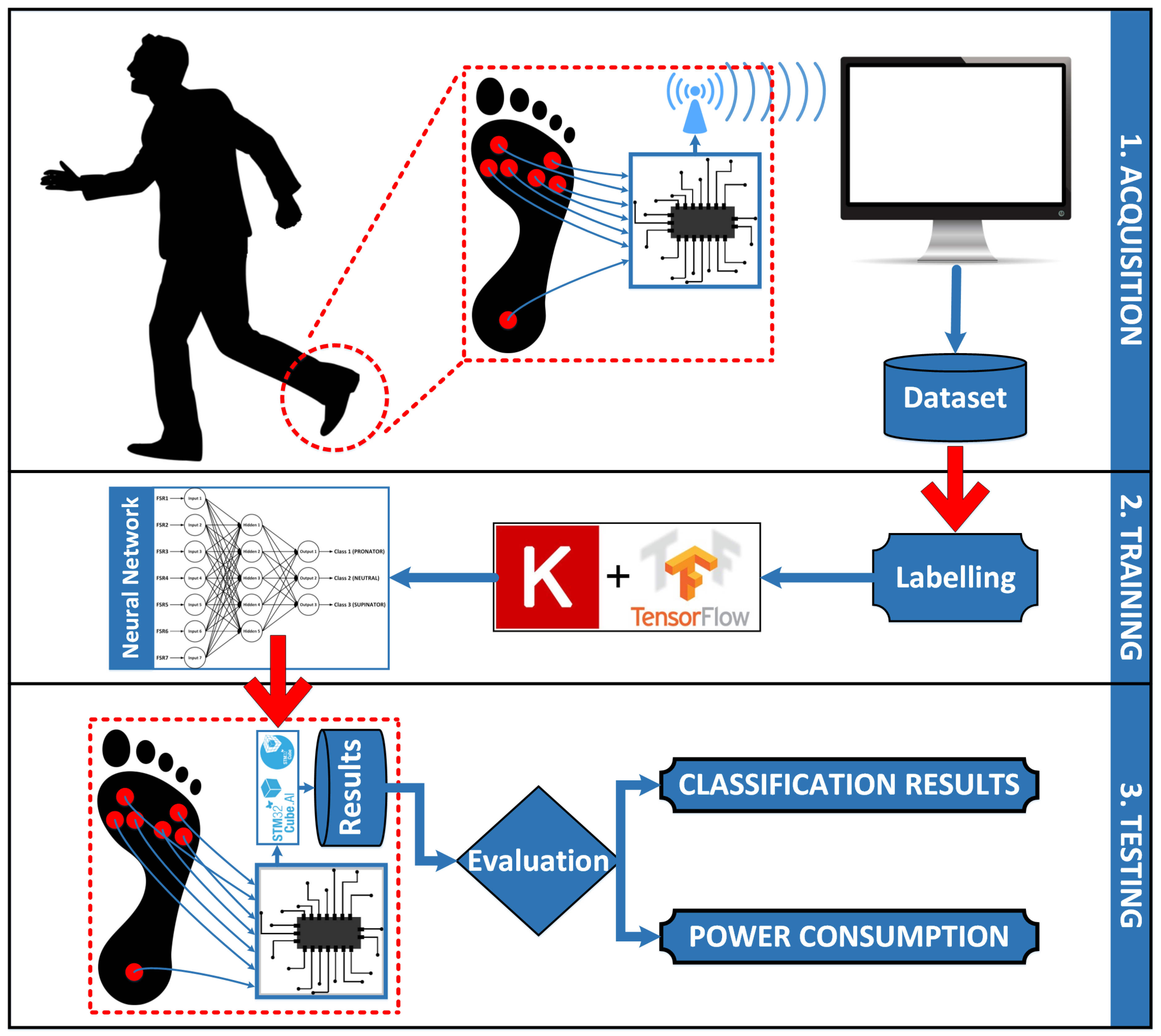
2. Materials and Methods
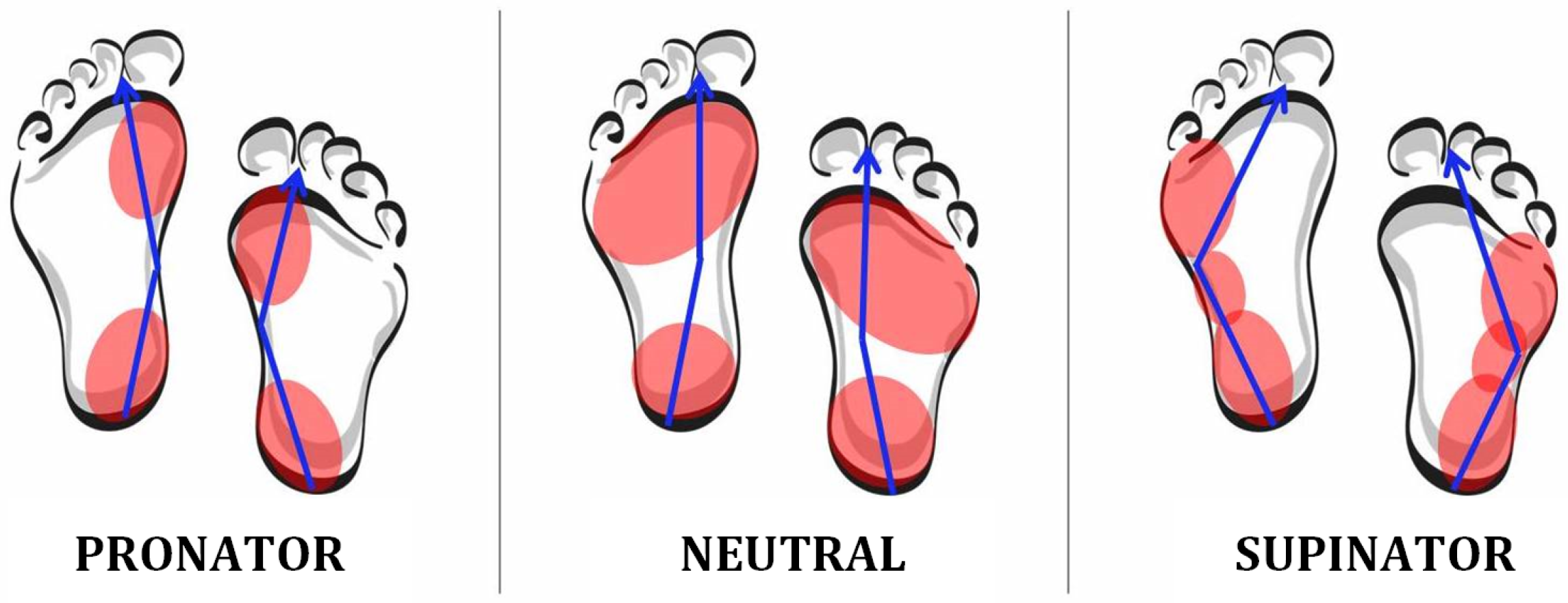
2.1. Data Acquisition
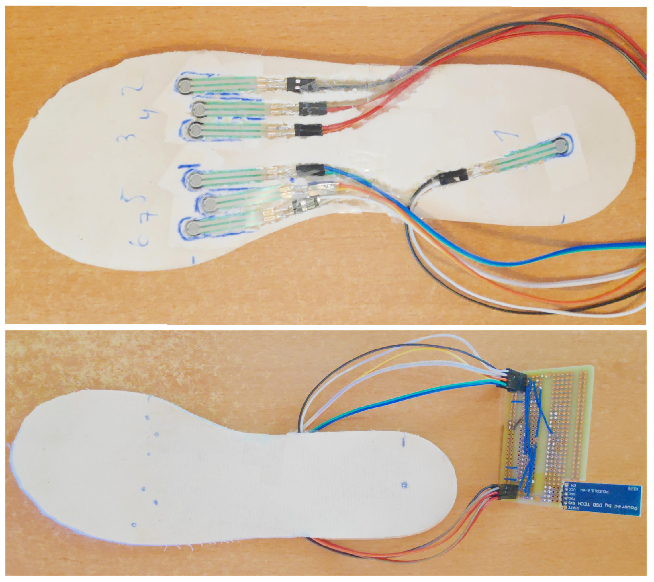
2.1.1. Footwear Insole
2.1.2. Dataset
2.2. Artificial Neural Network Classifier
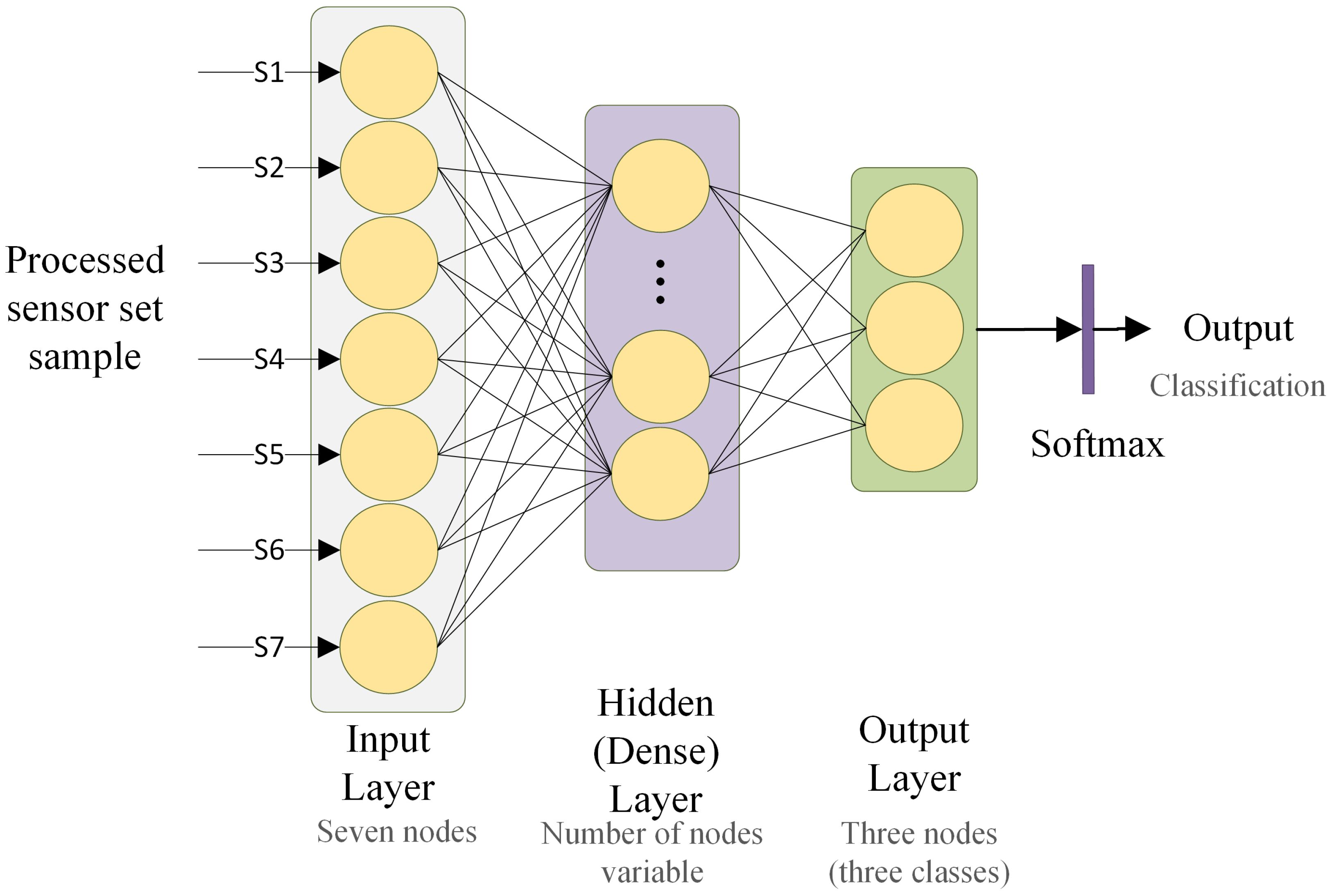
2.2.1. Architecture Design
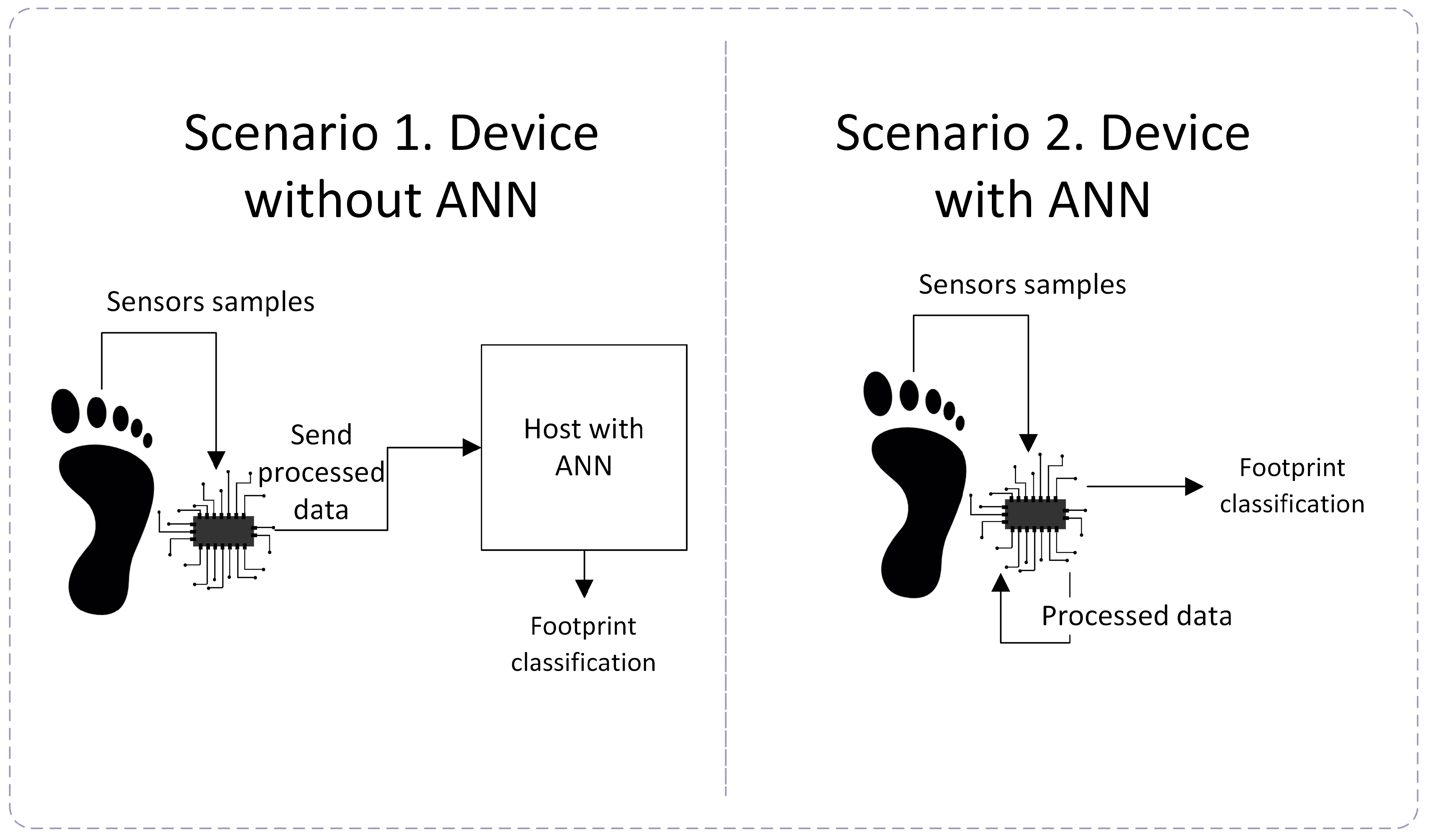
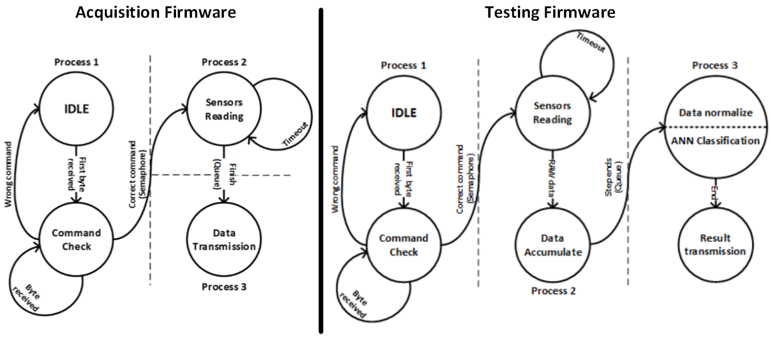
2.2.2. Embedded Model Analysis
3. Results and Discussion
3.1. Dataset
3.2. ANN Model Assessment
3.2.1. ANN Architectures and Parameters
3.2.2. Effectiveness Results
3.3. Embedded System Results
3.3.1. Embedded Model Accuracy
3.3.2. Execution Times
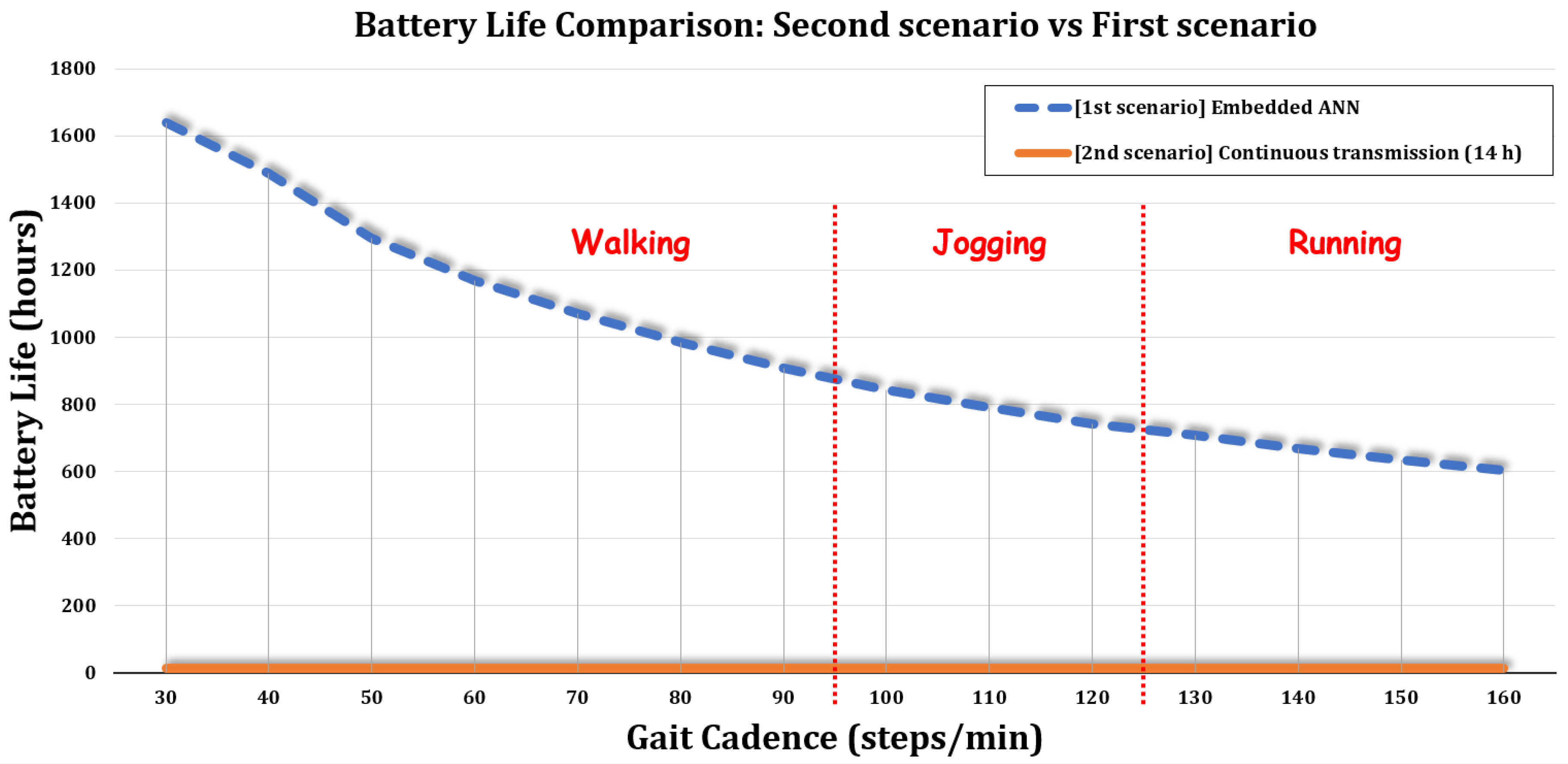
3.3.3. Power Consumption Analysis
4. Conclusions
Author Contributions
Funding
Acknowledgments
Conflicts of Interest
Abbreviations
| OS | Operating System |
| ANN | Artificial Neural Network |
| FSR | Force Sensitive Resistors |
| BLE | Bluetooth Low Energy |
| MCU | Microcontroller |
| ReLU | Rectified Linear Unit |
References
- Thomas, M.J.; Roddy, E.; Zhang, W.; Menz, H.B.; Hannan, M.T.; Peat, G.M. The population prevalence of foot and ankle pain in middle and old age: A systematic review. Pain 2011, 152, 2870–2880. [Google Scholar] [CrossRef]
- Menz, H.B. Chronic foot pain in older people. Maturitas 2016, 91, 110–114. [Google Scholar] [CrossRef] [PubMed]
- Menz, H.B.; Dufour, A.B.; Riskowski, J.L.; Hillstrom, H.J.; Hannan, M.T. Association of planus foot posture and pronated foot function with foot pain: The Framingham foot study. Arthritis Care Res. 2013, 65, 1991–1999. [Google Scholar] [CrossRef]
- Buldt, A.K.; Allan, J.J.; Landorf, K.B.; Menz, H.B. The relationship between foot posture and plantar pressure during walking in adults: A systematic review. Gait Posture 2018, 62, 56–67. [Google Scholar] [CrossRef] [PubMed]
- Perry, J.; Davids, J.R. Gait analysis: Normal and pathological function. J. Pediatr. Orthop. 1992, 12, 815. [Google Scholar] [CrossRef]
- Buldt, A.K.; Forghany, S.; Landorf, K.B.; Levinger, P.; Murley, G.S.; Menz, H.B. Foot posture is associated with plantar pressure during gait: A comparison of normal, planus and cavus feet. Gait Posture 2018, 62, 235–240. [Google Scholar] [CrossRef]
- Razeghi, M.; Batt, M.E. Foot type classification: A critical review of current methods. Gait Posture 2002, 15, 282–291. [Google Scholar] [CrossRef]
- Frelih, N.G.; Podlesek, A.; Babič, J.; Geršak, G. Evaluation of psychological effects on human postural stability. Measurement 2017, 98, 186–191. [Google Scholar] [CrossRef]
- Morris, S.J.; Paradiso, J.A. Shoe-integrated sensor system for wireless gait analysis and real-time feedback. In Proceedings of the Second Joint 24th Annual Conference and the Annual Fall Meeting of the Biomedical Engineering Society, Houston, TX, USA, 23–26 October 2002; Volume 3, pp. 2468–2469. [Google Scholar]
- Bamberg, S.J.M.; Benbasat, A.Y.; Scarborough, D.M.; Krebs, D.E.; Paradiso, J.A. Gait analysis using a shoe-integrated wireless sensor system. IEEE Trans. Inf. Technol. Biomed. 2008, 12, 413–423. [Google Scholar] [CrossRef]
- Shu, L.; Hua, T.; Wang, Y.; Li, Q.; Feng, D.D.; Tao, X. In-shoe plantar pressure measurement and analysis system based on fabric pressure sensing array. IEEE Trans. Inf. Technol. Biomed. 2010, 14, 767–775. [Google Scholar]
- Wahab, Y.; Mazalan, M.; Bakar, N.; Anuar, A.; Zainol, M.; Hamzah, F. Low power shoe integrated intelligent wireless gait measurement system. J. Phys. Conf. Ser. IOP Publ. 2014, 495, 13–14. [Google Scholar] [CrossRef]
- Crea, S.; Donati, M.; De Rossi, S.M.M.; Oddo, C.M.; Vitiello, N. A wireless flexible sensorized insole for gait analysis. Sensors 2014, 14, 1073–1093. [Google Scholar] [CrossRef] [PubMed]
- Talib, N.; Rahman, M.; Najib, A.; Noor, M. Implementation of Piezoelectric Sensor in Gait Measurement System. In Proceedings of the 2018 8th IEEE International Conference on Control System, Computing and Engineering (ICCSCE), Penang, Malaysia, 23–25 November 2018; pp. 20–25. [Google Scholar]
- Oshimoto, T.; Abe, I.; Kikuchi, T.; Chijiwa, N.; Yabuta, T.; Tanaka, K.; Asaumi, Y. Gait Measurement for Walking Support Shoes with Elastomer-Embedded Flexible Joint. In Proceedings of the 2019 IEEE/SICE International Symposium on System Integration (SII), Paris, France, 14–16 January 2019; pp. 537–542. [Google Scholar]
- Ngamsuriyaroj, S.; Chira-Adisai, W.; Somnuk, S.; Leksunthorn, C.; Saiphim, K. Walking gait measurement and analysis via knee angle movement and foot plantar pressures. In Proceedings of the 2018 15th International Joint Conference on Computer Science and Software Engineering (JCSSE), Nakhonpathom, Thailand, 11–13 July 2018; pp. 1–6. [Google Scholar]
- Dominguez-Morales, J.P.; Rios-Navarro, A.; Dominguez-Morales, M.; Tapiador-Morales, R.; Gutierrez-Galan, D.; Cascado-Caballero, D.; Jimenez-Fernandez, A.; Linares-Barranco, A. Wireless sensor network for wildlife tracking and behavior classification of animals in Doñana. IEEE Commun. Lett. 2016, 20, 2534–2537. [Google Scholar] [CrossRef]
- Henkel, J.; Pagani, S.; Amrouch, H.; Bauer, L.; Samie, F. Ultra-low power and dependability for IoT devices (Invited paper for IoT technologies). In Proceedings of the Design, Automation & Test in Europe Conference & Exhibition (DATE), Lausanne, Switzerland, 27–31 March 2017; pp. 954–959. [Google Scholar]
- Andres-Maldonado, P.; Ameigeiras, P.; Prados-Garzon, J.; Ramos-Munoz, J.J.; Lopez-Soler, J.M. Optimized LTE data transmission procedures for IoT: Device side energy consumption analysis. In Proceedings of the 2017 IEEE International Conference on Communications Workshops (ICC Workshops), Paris, France, 21–25 May 2017; pp. 540–545. [Google Scholar]
- Deepu, C.J.; Heng, C.H.; Lian, Y. A hybrid data compression scheme for power reduction in wireless sensors for IoT. IEEE Trans. Biomed. Circuits Syst. 2016, 11, 245–254. [Google Scholar] [CrossRef]
- Domínguez-Morales, M.J.; Luna-Perejón, F.; Miró-Amarante, L.; Hernández-Velázquez, M.; Sevillano-Ramos, J.L. Smart Footwear Insole for Recognition of Foot Pronation and Supination Using Neural Networks. Appl. Sci. 2019, 9, 3970. [Google Scholar] [CrossRef]
- Pineda-Gutiérrez, J.; Miró-Amarante, L.; Hernández-Velázquez, M.; Sivianes-Castillo, F.; Domínguez-Morales, M. Designing a Wearable Device for Step Analyzing. In Proceedings of the 2019 IEEE 32nd International Symposium on Computer-Based Medical Systems (CBMS), Cordoba, Spain, 5–7 June 2019; pp. 259–262. [Google Scholar]
- Anderson, D.; McNeill, G. Artificial neural networks technology. Kaman Sci. Corp. 1992, 258, 1–83. [Google Scholar]
- Luna-Perejón, F.; Domínguez-Morales, M.J.; Civit-Balcells, A. Wearable Fall Detector Using Recurrent Neural Networks. Sensors 2019, 19, 4885. [Google Scholar] [CrossRef]
- Nasser, I.M.; Abu-Naser, S.S. Lung Cancer Detection Using Artificial Neural Network. Int. J. Eng. Inf. Syst. 2019, 3, 17–23. [Google Scholar]
- Sadek, R.M.; Mohammed, S.A.; Abunbehan, A.R.K.; Ghattas, A.K.H.A.; Badawi, M.R.; Mortaja, M.N.; Abu-Nasser, B.S.; Abu-Naser, S.S. Parkinson’s Disease Prediction Using Artificial Neural Network. Int. J. Acad. Health Med. Res. 2019, 3, 1–8. [Google Scholar]
- Gutierrez-Galan, D.; Dominguez-Morales, J.P.; Cerezuela-Escudero, E.; Rios-Navarro, A.; Tapiador-Morales, R.; Rivas-Perez, M.; Dominguez-Morales, M.; Jimenez-Fernandez, A.; Linares-Barranco, A. Embedded neural network for real-time animal behavior classification. Neurocomputing 2018, 272, 17–26. [Google Scholar] [CrossRef]
- Sheela, K.G.; Deepa, S.N. Review on methods to fix number of hidden neurons in neural networks. Math. Probl. Eng. 2013, 2013, 425740. [Google Scholar] [CrossRef]
- Sokolova, M.; Lapalme, G. A systematic analysis of performance measures for classification tasks. Inf. Process. Manag. 2009, 45, 427–437. [Google Scholar] [CrossRef]
- Finnoff, W.; Hergert, F.; Zimmermann, H.G. Improving model selection by nonconvergent methods. Neural Netw. 1993, 6, 771–783. [Google Scholar] [CrossRef]
- Tudor-Locke, C.; Aguiar, E.J.; Han, H.; Ducharme, S.W.; Schuna, J.M.; Barreira, T.V.; Moore, C.C.; Busa, M.A.; Lim, J.; Sirard, J.R.; et al. Walking cadence (steps/min) and intensity in 21–40 year olds: CADENCE-adults. Int. J. Behav. Nutr. Phys. Act. 2019, 16, 1–11. [Google Scholar] [CrossRef]


| Subset | Neutral | Pronator | Supinator | Total |
|---|---|---|---|---|
| Total | 1067 | 1129 | 928 | 3124 |
| Training | 917 | 955 | 784 | 2656 |
| Test | 150 | 174 | 144 | 468 |
| Nodes in Hidden Layer | Accuracy | Precision | F1-Score | Specificity | Sensitivity |
|---|---|---|---|---|---|
| Five nodes | 0.987 | 0.987 | 0.994 | 0.987 | 0.987 |
| Four nodes | 0.994 | 0.994 | 0.997 | 0.994 | 0.994 |
| Three nodes | 0.996 | 0.996 | 0.998 | 0.996 | 0.996 |
| Two nodes | 0.991 | 0.992 | 0.996 | 0.992 | 0.992 |
| One node | 0.678 | 0.653 | 0.842 | - | - |
| Nodes in Hidden Layer | Not-Compressed | ×4 Compression | ×8 Compression |
|---|---|---|---|
| Five nodes | 6.816 | ||
| Four nodes | |||
| Three nodes | |||
| Two nodes | |||
| One node |
| Nodes in Hidden Layer | Not-Compressed | Compression | Compression |
|---|---|---|---|
| Five nodes | 0.071 | 0.071 | 0.075 |
| Four nodes | 0.067 | 0.067 | 0.070 |
| Three nodes | 0.061 | 0.061 | 0.061 |
| Two nodes | 0.056 | 0.056 | 0.056 |
| One node | 0.052 | 0.052 | 0.052 |
| Cadence (Steps/min) | Sec. Spent for Each Step | # Samples for Each Step (1 foot) | Tx Power Consumption for Each Reading (A) | System Average Consumption (A) | Battery Life (h) |
|---|---|---|---|---|---|
| 30 | 2.00 | 50.00 | 0.86 | 75.11 | 1639 |
| 40 | 1.50 | 37.50 | 1.15 | 85.26 | 1488 |
| 50 | 1.20 | 30.00 | 1.44 | 95.41 | 1297 |
| 60 | 1.00 | 25.00 | 1.73 | 105.57 | 1171 |
| 70 | 0.86 | 21.43 | 2.01 | 115.37 | 1071 |
| 80 | 0.75 | 18.75 | 2.30 | 125.53 | 984 |
| 90 | 0.67 | 16.67 | 2.59 | 135.68 | 909 |
| 100 | 0.60 | 15.00 | 2.88 | 145.84 | 845 |
| 110 | 0.55 | 13.64 | 3.17 | 155.64 | 792 |
| 120 | 0.50 | 12.50 | 3.45 | 165.80 | 743 |
| 130 | 0.46 | 11.54 | 3.74 | 175.95 | 709 |
| 140 | 0.43 | 10.71 | 4.03 | 186.11 | 670 |
| 150 | 0.40 | 10.00 | 4.32 | 196.26 | 636 |
| 160 | 0.38 | 9.38 | 4.60 | 206.06 | 605 |
© 2020 by the authors. Licensee MDPI, Basel, Switzerland. This article is an open access article distributed under the terms and conditions of the Creative Commons Attribution (CC BY) license (http://creativecommons.org/licenses/by/4.0/).
Share and Cite
Luna-Perejón, F.; Domínguez-Morales, M.; Gutiérrez-Galán, D.; Civit-Balcells, A. Low-Power Embedded System for Gait Classification Using Neural Networks. J. Low Power Electron. Appl. 2020, 10, 14. https://doi.org/10.3390/jlpea10020014
Luna-Perejón F, Domínguez-Morales M, Gutiérrez-Galán D, Civit-Balcells A. Low-Power Embedded System for Gait Classification Using Neural Networks. Journal of Low Power Electronics and Applications. 2020; 10(2):14. https://doi.org/10.3390/jlpea10020014
Chicago/Turabian StyleLuna-Perejón, Francisco, Manuel Domínguez-Morales, Daniel Gutiérrez-Galán, and Antón Civit-Balcells. 2020. "Low-Power Embedded System for Gait Classification Using Neural Networks" Journal of Low Power Electronics and Applications 10, no. 2: 14. https://doi.org/10.3390/jlpea10020014
APA StyleLuna-Perejón, F., Domínguez-Morales, M., Gutiérrez-Galán, D., & Civit-Balcells, A. (2020). Low-Power Embedded System for Gait Classification Using Neural Networks. Journal of Low Power Electronics and Applications, 10(2), 14. https://doi.org/10.3390/jlpea10020014