Efficient and Equitable Climate Change Policies

Abstract

This report describes the Integrated Assessment Model TIAM-MACRO, which is a Ramsey-type macroeconomic growth model linked with a technology-rich engineering model of the energy-system and with a stylized sub-model of climate change. TIAM-MACRO contributes to coherent and consistent policy analyses at both the world and regional level and correlates demand for energy services to macro-economic developments across regions and time until the end of the 21st century. With the help of this model, two contrasting scenarios are defined related to the reference development (BASE) case and the 2 °C (2DS) case that follow long-term policies on climatic change mitigation in the spirit of the Paris agreement. Finally, we define ex-post market and non-market damages together with the damages related to Local Atmospheric Pollutants (LAP). The stringency of the 2DS case requires the complete restructuring of the energy and transport systems to be relying on carbon-free technologies and fuels together with technologies of negative emissions, at high costs. The study concludes that carbon policies not only consist of an insurance against the risk of climate change but also improve the ambient air quality, as they have secondary benefits that compensate for part of the cost of carbon control. However, the stringency of the 2DS case is so demanding that the cost of climate policies is above benefits.

1. Introduction

The energy oil crisis of the last century has inspired the development of different modelling schools and their energy-related specific software tools for policy analysis (such as Agent-Based models, Applied General Equilibrium models, System Dynamics models, Integrated Assessment Models based on Mathematical Programming (MP), Game theoretical models, and Multi Criteria Decision Making Analysis approaches). TIAM-MACRO represents one such development that has taken place in the course of the last 50 years under the aegis of the International Energy Agency, Energy Technology Systems Analysis Program (IEA-ETSAP). Based on MP and general equilibrium methods, it has a consistent analytical capability in the fields of energy, economy, environment, and engineering (4E). The development of the energy systems resources described in TIAM-MACRO and their transformation to different forms of final energy commodities satisfying end-use sectors demands is a key determinant of sustainability as it prescribes energy and economic efficiency and local and global environmental emissions and damages, drives economic development, and has consequences on the social wellbeing of humanity. Furthermore, the sustainability dimension in economic growth is further pronounced in some versions of the model, where the sectors of Agriculture, Forestry, and Land Use are either expanded directly in TIAM to assess water, energy, and land use and include food, biomass, and forest products [1]. Alternatively, the energy models are integrated with global biomass/biosphere management systems, such as MESSAGE-GLOBIOM [2], REMIND-MAgPIE [3], and WITCH-GLOBIOM [4]. The different aspects of resource assessment processes modelled by the IEA-ETSAP consortium address actual policy questions that need a holistic approach and integration in the same framework.

This general equilibrium growth modelling platform of TIAM-MACRO [5] is consistent with other global energy modelling tools based on mathematical programming [6,7,8,9] and extends the geographical coverage of the 4E methodology at the national, regional, and global level with 15 world regions. The model evaluations support decision-making analysis and the formulation of suitable operative strategies. It integrates the most important LAP externalities and damage functions, together with the damages of climate change, and allows for the performance of cost/benefit (CBA) and second best analysis (SBA) identifying appropriate technological options and prioritizing measures for cost-efficient energy systems. The model is applied either directly for the assessment of economic efficiency and equity considerations in its deterministic version or is extended to consider stochastic and/or probabilistic risk assessment principles related to climate change and other policies.

The previous studies done with the global TIAM model were partial equilibrium applications not able to define macroeconomic consumption (and gross domestic product, GDP) losses or the primary and secondary benefits of climate policy. Therefore, the assessment of burden sharing rules done in the past with TIAM were incomplete.

Overall, this paper: (a) analyses the global energy system under economically efficient policies; (b) incorporates an evaluation of climate benefits (reduction of climate change damages) together with the co-benefits of improved ambient air quality; (c) describes a unique methodology for the regionalization of external cost valuation of local air pollution; and (d) applies burden sharing rules under efficiency and equity considerations and proposes a rule balancing the interest of North and South for the implementation of the Paris agreement. This article describes first in Section 2 the techno-economic model TIAM-MACRO and continues with the scenario specification (Section 3). Then, some recent applications related to climate change and local atmospheric pollution are described (Section 4 and Section 5). Section 6 performs ex-post analysis for efficient and equitable scenarios, while Section 7 derives the main conclusions of the study and highlights future modelling directions for the assessment of climate change.

2. The Energy Model TIAM

2.1. The Reference Energy System (RES)

The definition of RES is the first decision concerning the level of detail and the structure of model specifications. The RES in TIAM includes the followings sectors: Residential, Commercial, Agriculture, Industry, Transportation, Electricity/Heat production, and Energy Supply. In particular, the structure of the RES identifies the demand categories energy carriers, emissions, and materials, in brief:

Transportation includes road and rail for passengers and freight, navigation, and aviation. In road transport, there are five demand categories for passenger travel (cars: short distance, cars: long distance, buses: urban, buses: intercity, and two and three-wheelers/off road) and trucking. In rail transport, there are three demand categories (passengers: light trains (metros), passengers: heavy trains, and rail freight). The aviation and navigation sectors are modelled using a single generic technology each and a single generic demand each that reproduces the energy consumption. In Residential, there are different end-uses (Space heating, Space Cooling, Water heating, Cooking, Lighting, Refrigeration, Cloth washing, Cloth drying, Dish Washing, Other electric, and Other energy), and the first three are differentiated by building categories (Single house: rural, Single house: urban, and Multi Apartment). Similarly, the RES structure of the Commercial sector has nine end-uses (Space heating, Space Cooling, Water heating, Cooking, Refrigeration, Lighting, Public Lighting, Other electric, and Other Energy Uses), with the first three being differentiated by building categories (Small/Large). Agriculture is modelled as a single generic technology with a mix of fuels as input and an aggregated useful energy demand as output, while in some applications the sector is expanded to include food, biomass, and forestry. Industry is divided into two different sets: energy-intensive industries and other industries. For the energy-intensive industries (steel, cement, chemical, and non-ferrous metals), explicit existing and alternative processes have been modeled, i.e., using data at regional level, whereas for other industries a standard structure consisting in a mix of five main energy uses (Steam, Process heat, Machine drive, Electrochemical, and Other processes) was adopted.

In order to start moving in the direction of Life Cycle Assessment (LCA), different material demands of the industrial sector (as for example steel or limestone) were modelled separately. Electricity and Heat production: this sector regroups public power plants, auto production of electricity, and Combined Power and Heat (CHP). In the RES, three types of electricity (High voltage, Medium voltage, and Low voltage) and two separated (not connected) grids for long distance (high temperature) and short distance (low temperature) heat are distinguished. Supply: Each primary resource (Crude Oil, Natural Gas, Hard coal, and Lignite) is modelled by a supply curve with several cost steps. There are three categories of sources: located reserves (or producing pools), reserves growth (or enhanced recovery), and new discovery. In addition, five types of biomass are modelled: wood products, biogas, municipal waste, industrial waste-sludge, and biofuels. Energy carriers were chosen starting from those reported in the IEA energy balances [10] and then aggregating some of them to adapt the list to the modelling objectives of the project. Only energy-intensive processes (e.g., scrap steel) are explicitly modeled. Other materials are implicitly modelled as part of the variable costs and their related emissions accounted for in the process emissions. The air emissions modelled are Carbon Dioxide (CO₂), Methane (CH₄), Sulphur dioxide (SO₂), Nitrogen Oxides (NOx), Nitrous Oxide (N₂O), Particulate Matter (PM2.5 and PM10), and Volatile Organic Compounds (VOC).

The model describes the time evolution of the energy systems, from primary energy resources to end-use devices, by sector. Energy, material, and emissions balances as well as operation and maintenance cost together with investment costs are generated for each scenario, region, and time. This information is processed in the report generator to define different indicators, such as energy efficiency, energy intensity, carbon intensity, and emissions per capita.

2.2. Technology Data

Energy commodities include a full spectrum of resource potentials and their costs for fossil fuels, nuclear, bioenergy, and both traditional and modern renewable technologies. Since the TIAM model is an integrated techno-economic energy model, its database includes technologies in all transformation sectors of the economy, namely: primary energy extraction, energy processing and conversion, energy transport, and end-uses. Thus, the TIMES database presented in the homepage of the IEA/ETSAP project [11] will concern more than a thousand technologies in each country/region model. In addition, the global model represents the main energy exchanges between world regions, where each energy trade is modelled via a trade technology (pipeline, trucking, shipping, transmission grid). TIAM independently calculates a dynamic inter-temporal partial equilibrium on global energy and emissions markets based on a minimization of the total discounted energy system cost with perfect foresight to 2100 [12,13].

2.3. LAP Emissions and External Costs

The difference in the approach applied in TIAM, in relation to other studies considering LAP emissions and externalities [14,15,16],1 is that TIAM includes a direct valuation of externalities in its database that defines the specific damages per unit of pollutant while the other studies follow the causality chain, e.g., they start from emissions sources to atmospheric dispersion and chemistry models to define concentrations of pollutants and perform the economic valuation of damages.

The TIAM methodology developed for deriving specific external-cost factors of LAP emissions for all of the world’s regions is presented in [17] and is based on the initial specific external cost factors evaluated for each pollutant for Europe in the “New Energy Externalities Developments for Sustainability” (NEEDS) [18] project. The method adjusts the NEEDS values for Europe to the rest of the 14 world regions (regionalization) and projects them into the future. The regionalization follows the willingness-to-pay (WTP) principle for clean air and the population density, with different elasticities for the industrialized world and the developing countries. Then, the GDP uplift factor takes into account the development of the WTP in the TIAM regions that follow GDP growth with an elasticity and an urbanization factor related to the growth in population density. The four factors, i.e., WTP, population density, GDP uplift, and urbanization, are multiplied to find the total (combined) adjustment factor per region and time.

Furthermore, the regional calibration of specific emissions for the year 2005 follows the emissions inventory guidebook [19], the regional LAP emissions balances given by activity in the European database EDGAR [20], and the IEA energy statistics by region, sector, and demand category. Future emissions for new technologies by sector are partially exogenous assumptions:

• Power Sector. Emissions for each technology follow either the NEEDS data with end-of-pipe measures included in the cost, or the U.S. Environmental Protection Agency (EPA) data [21] for the missing NEEDS technologies.
• Transport. The transport sector is quite detailed and is based on NEEDS for each technology, explicitly following model activities rather than being on a fuel-consumption basis.
• In all other sectors, the calibrated emission coefficients for the base year take into account exogenous future improvement via policies and end-of-pipe technologies and are generic. In the reference development (BASE) scenario presented in this report, emission coefficients in 2020 are lower by 10% relative to 2005, by 20% in 2030, by 30% in 2050, and by 55% in 2100. In addition, extra desulfurization measures in the industrial sectors of China and India are implemented. This approach simulates emission standards following technological change without extra investment costs in the model (see also [15] for scenario PROG, where specific emission reductions are defined between stabilization in the levels of 2010 and the best possible available technology).

2.4. Macro Stand Alone (MSA)

Before going to the description of the Macroeconomic module, we introduce the demand equation for energy services of TIAM. The ETSAP family of models defines first demands that reflect past trends and exogenous assumptions on population, GDP, and energy intensity based on the evolution of demand drivers and their elasticities. As most of the efficiency improvement options are included in the engineering model explicitly, and are selected if they make economic sense, the autonomous efficiency improvement factors (aeeif) applied below could be introduced to reflect mainly lifestyle changes. The relation for demand projections is the following:

$$\frac{D_{it}}{D_{i0}}={\left[\frac{d{r}_{it}}{d{r}_{io}}\right]}^{{\alpha }_i}\cdot {\left[\frac{P_{it}}{P_{i0}}\right]}^{-{\sigma }_i}\cdot {\displaystyle \prod _{\tau =1,t}{(1-aeei{f}_{i\tau })}^{yp{p}_{\tau }}}.$$

(1)

Here, Dit/Di₀ is the relative demand projection for sector i and period t normalized to the demand for the starting year, which is calibrated to energy statistics in line with the efficiencies of the end-use devices valid in the starting year of analysis; dr_it is the demand driver; α_it the driver elasticity; σ_t the price elasticity; aeeif_it the autonomous efficiency improvement factor per demand category; ypp_τ the years per period; and Pit/Pi₀ the index of relative demand prices. TIAM (the global and multiregional version of TIMES) assumes different growth rates and elasticities of demand drivers for each individual demand category. Usually, some consistency checks of economic assumptions and the projections generated based on the equation above must be completed. IIASA, for example, adjusts projections to the results of MERGE [22], while ETSAP uses GEM-E3 [23]. The model calibration starts with the year 2005 and reproduces the energy balances of the IEA. Calibration extends to the future for the Baseline and reproduces the demands for energy services by region and time (Equation (1)). This over-time calibration of TIAM is obtained with the specification of the demand decoupling factors (ddf) of Equation (10).

The macroeconomic module MSA is a Ramsey-type growth model and defines the demand for energy services of TIAM. Total economic production is determined as a constant elasticity of substitution function of the energy construct and the value-added pair of capital and labor, where energy substitutes with the capital–labor composite via an elasticity of substitution, Equation (4) decomposing the energy system solution into a quadratic cost function (Equation (8)) and to price responsive demand decoupling factors (Equations (1) and (7)) that establish the coupling link between TIAM and MSA.

MSA supports multiple regions maximizing the Negishi-weighted sum of regional utilities (Equation (2)), while TIAM-MACRO is solved iteratively in a sequence of optimizations starting with the solution of the standard TIAM model. This defines a quadratic cost function of the energy system (Equation (8)) for use in the stand-alone MSA model, which is then solved by maximizing utility (Equation (2)) and redefines the demand for energy services (Equations (4) and (7)). At the end of the iterations, and when equilibrium is obtained (within a 10^–5 error margin), the climate module is called to define concentrations of greenhouse gases (GHGs), climate forcing, and temperature change.2

The MSA model considers only the trade of the numéraire good (Equation (9)), as all other traded energy products are established in TIAM. Equation (3) distributes the economic output (Y) to consumption (C) and capital investments (INV) and supports the energy system costs (EC) while Equation (5) defines the depreciation of capital. Finally, Equation (11) reflects the exogenous development of the labor force index that follows the economic growth rate.

The basic formulation of MSA in period t and region r follows Equations (2)–(11):

$$MaxU={\displaystyle \sum _{t=1}^T{\displaystyle \sum _{r}nw{t}_r\cdot pw{t}_t\cdot dfac{t}_{r,t}\cdot \ln (C_{r,t})}}$$

(2)

$$Y_{r,t}=C_{r,t}+IN{V}_{r,t}+E{C}_{r,t}+NTX{(nmr)}_{r,t}$$

(3)

$$Y_{r,t}={\left(ak{l}_r\cdot K_{r,t}^{kpv{s}_r\cdot {\rho }_r}\cdot l_{r,t}^{(1-kpv{s}_r){\rho }_r}+{\displaystyle \sum _k{b}_{r,k}\cdot DE{M}_{r,t,k}^{{\rho }_r}}\right)}^{\frac{1}{{\rho }_r}}$$

(4)

$$K_{r,t+1}=tsr{v}_{r,t}\cdot K_{r,t}+\frac{1}{2}(d_t\cdot tsr{v}_{r,t}\cdot IN{V}_{r,t}+d_{t+1}\cdot IN{V}_{r,t+1})$$

(5)

$$K_{r,T}\cdot (grow{v}_{r,T}+dep{r}_r)\le IN{V}_{r,T}$$

(6)

$$DE{T}_{r,t,k}=aeeifa{c}_{r,t,k}\cdot DE{M}_{r,t,k}$$

(7)

$$E{C}_{r,t}=q{a}_{r,t}+{\displaystyle \sum _{k}q{b}_{r,t,k}\cdot {(DE{T}_{r,t,k})}^2}+am{p}_{r,t}$$

(8)

$${\displaystyle \sum _{r}NTX{(trd)}_{r,t}=0\hspace{1em}}\forall \{t,trd\}$$

(9)

$$aeeifa{c}_{r,t,k}={\displaystyle \prod _{\tau =1}^t{(1-dd{f}_{r,\tau ,k})}^{\frac{d_t+d_{t+1}}{2}}}$$

(10)

$$l_{r,1}=1\hspace{1em}\mathrm{and}\hspace{1em}{l}_{r,t+1}=l_{r,t}\cdot {(1+grow{v}_{r,t})}^{\frac{d_t+d_{t+1}}{2}}$$

(11)

where

• C_r,t: annual consumption (variable)
• Y_r,t: annual production (variable)
• K_r,t: total capital (variable)
• INV_r,t: annual investments (variable)
• DEM_r,t,k: annual demand in Macro for commodity k (variable)
• DET_r,t,k: annual demand in TIMES for commodity k (variable)
• EC_r,t: annual energy system costs in Macro (variable)
• Akl_r: production function constant
• amp_r,t: constant term to account for the full annualized investment cost of existing capacities in the starting period.
• B_r,k: demand coefficient for demand commodity k
• aeeifac_r,t,k: autonomous energy efficiency improvement
• d_t: duration of period t in years
• ddf_r,t,k demand decoupling factor (calibration parameter)
• depr_r: depreciation rate
• dfact_r,t: utility discount factor
• growv_r,t: growth rate (calibration parameter)
• kpvs: capital value share
• l_r,t: annual labor growth index
• nwt_r: Negishi weight for region r
• pwt: period-length-dependent weights in the utility function (these multipliers are introduced to in cases where the period lengths are not equal)
• qa_r,t: constant term of the quadratic supply cost function
• qb_r,t,k: coefficient for demand k in the quadratic supply cost function
• tsrv_r,t: capital survival factor between periods t and t + 1
• ρ_r: substitution constant
• T: number of periods in the model horizon

3. Scenarios Analyzed

The general idea for scenario analysis is to first build a Reference Scenario where all demand drivers are consistent with the assumptions used in similar projects by international organizations (IEA, EIA, and IIASA). Then, the model solves for the Reference development defining the evolution of the energy systems and the traded products to satisfy the exogenous demands for energy services while maximizing the global welfare. In all other scenarios, the initial macroeconomic assumptions, such as population and potential economic growth, are those of the reference scenario and are adjusted when the utility function is maximized under the CO₂ budget constraint. Thus, we conclude that the reference development is a reflection of the socioeconomic and energy intensity assumptions, while the policy development, which is the main model output, defines all needed changes to satisfy the imposed constraint.

In a study that demonstrates key characteristics of the model, we investigate two basic scenarios with TIAM-MACRO:

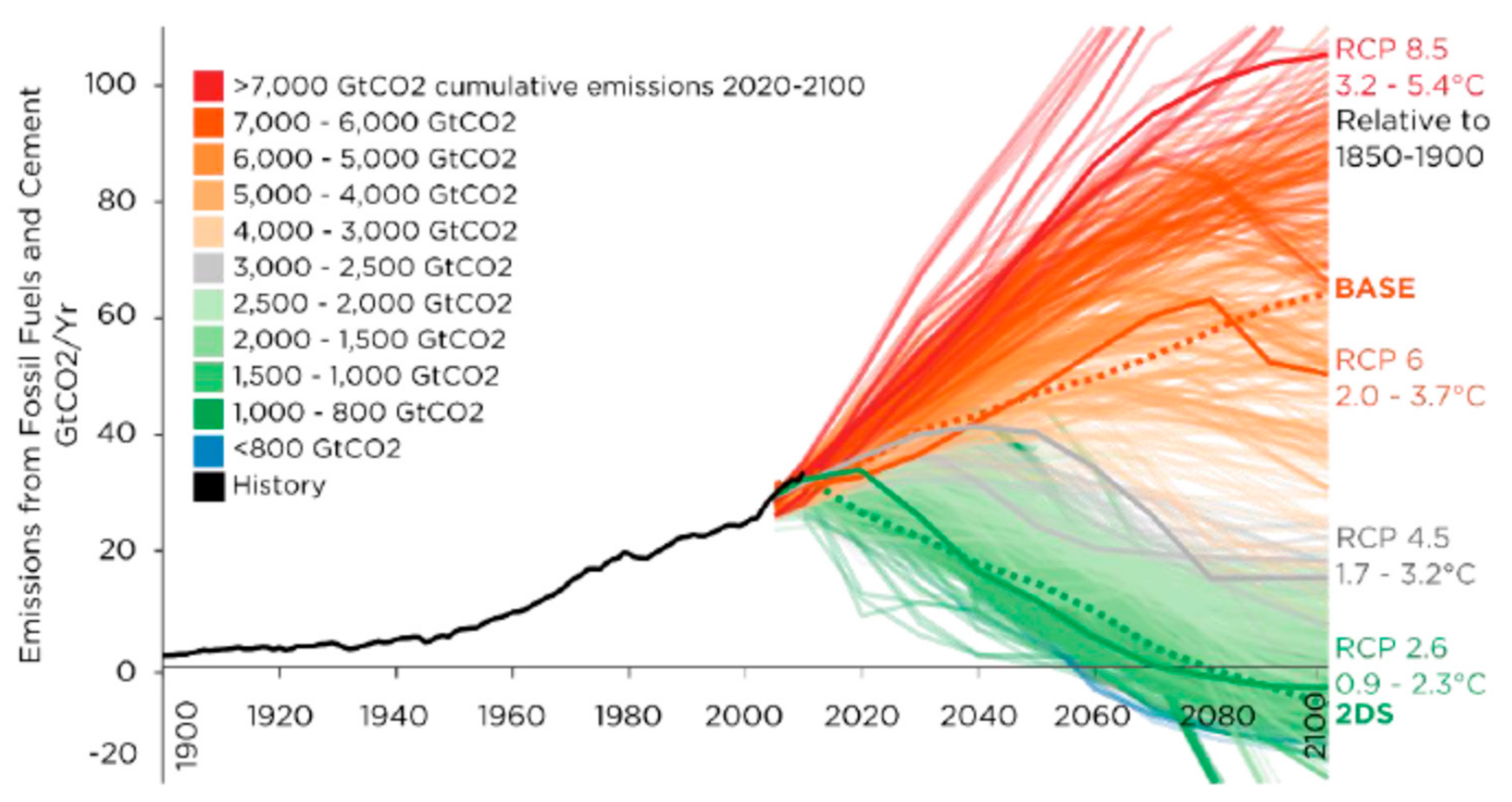
• The reference scenario (BASE) generated in the ETSAP project refers to the calibration year of 2005, describes the development of the global energy system in agreement with all other valid policies (including the nuclear phase out where it has been decided), and provides a baseline for comparing policy scenarios. The “BASE” scenario solves for least cost predicated on available resources and technologies under existing macroeconomic projections, which are consistent with the projections of the GEM-E3 [23] growth model. Total CO₂ emissions related to energy and cement production are similar to the short-term reductions resulting from the National Determined Contributions (NDCs) and follow the pathways of the Representative Concentration Pathways (RCP) 4.5 scenario up to 2030 (Figure 1). The BASE case economic projection does not take into account environmental damage costs to ecosystem services in the global economy due to climate change or health and other damages related to local atmospheric pollutants (LAP).
• Then, we assess the 2 °C (2DS) climate policy postulating a global cumulative CO₂eq budget compatible with the long-term target of 2 °C. The 2DS scenario begins with the same macroeconomic structure as the BASE scenario and a cumulative GHG budget of 1850 GtCO₂eq applied between 2020 and 2100 with a 50% confidence level to remain below 2 °C [24]. The emissions of the 2DS case, shown in Figure 1, are initially below those of the RCP2.6 case, which are starting to fall in 2020. The 2DS trajectory intercepts the RCP2.6 case in 2040, and follows a higher path afterwards to join again this trajectory at the end of the time horizon such that both integrals of emissions are quite the same.
• Finally, we define ex-post damages related to climate change and to the ambient air pollution for each scenario such that their differences (reduction of climate damages) and co-benefits (reduction of LAP damages) induced by climate policies are defined as the net benefits of the 2DS case over the BASE case. The cost of such policy (GDP losses of the 2DS scenario relative to BASE) is also evaluated, while this ex-post assessment presents a kind of alternative cost/benefit analysis.

4. Main Results and Discussion

The scenario analysis reflects the importance of utilizing an integrated modeling framework for climate and energy policy that includes the whole energy system and takes into account the trade-offs in a consistent way. Some of the most representative results derived from scenario analysis are presented in the following sections. The first results of this work were presented at the International Energy Workshop in Cork, Ireland in 2016 [25]. The present article presents revised scenarios and burden sharing results together with the contribution of emission sources not included in the first study, such as International Bunkers and industrial processes. In addition, we assume moderate but effective policies for controlling SO₂ emissions in the industrial processes of China and India.

4.1. Emission Pathways

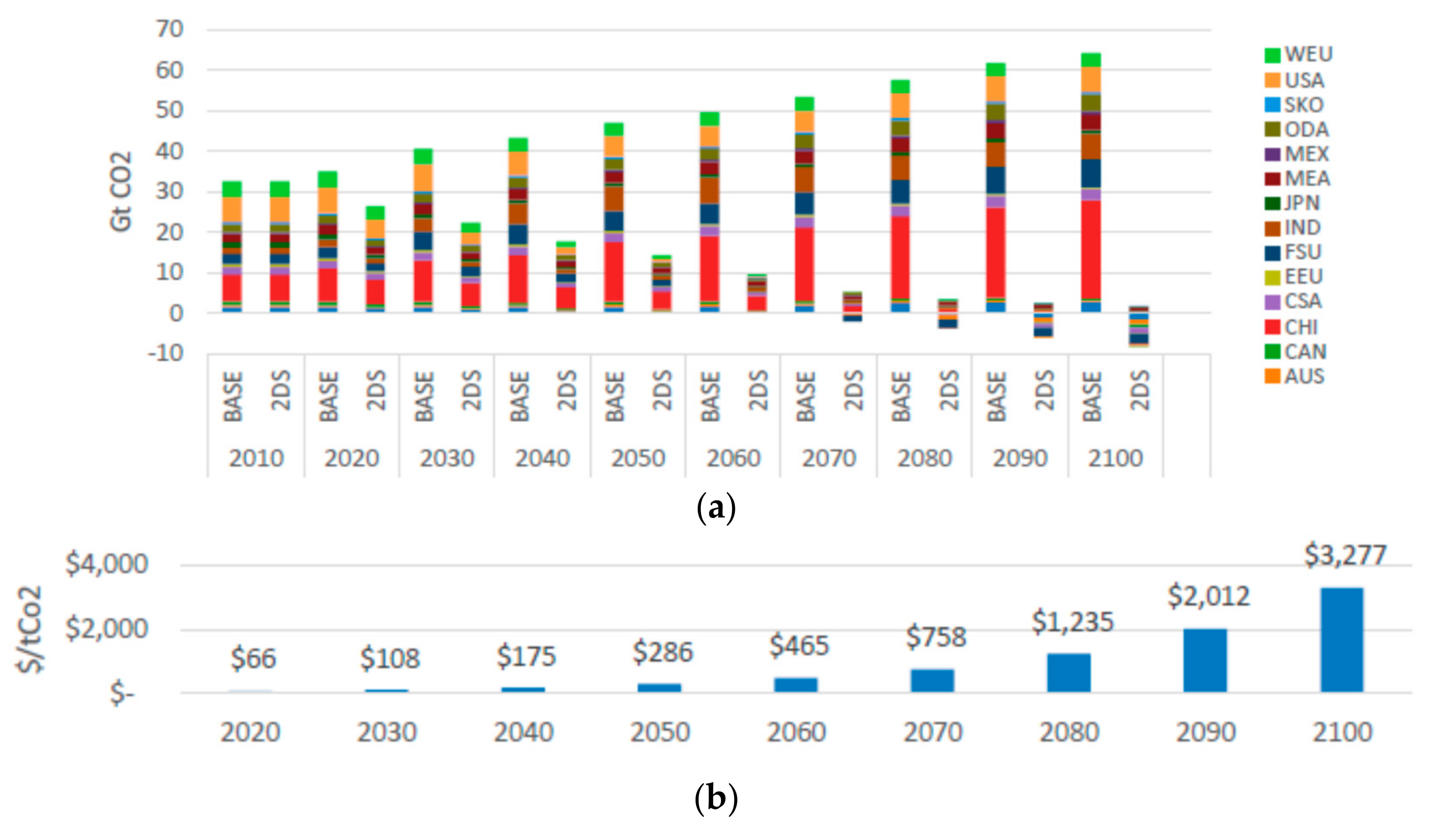
The emission pathways for the reference development (BASE) and the 2 °C cases are given in Figure 2a. Emissions in the BASE case are continuously increasing to reach a level of 64.2 GtCO₂ by the end of the century. In the 2 °C scenario (2DS), emission trajectories are reversed immediately with annual emission to be halved by 2030 and remain below 15 GtCO₂ beyond 2050. This is a consequence of the budget constraint applied between 2020 and 2100. Delayed action to after 2020 makes solving for a feasible solution increasingly difficult and at a larger abatement cost, considerably so towards the end of the horizon [26]. Significant long-term growth in capacity for renewable electricity and bioenergy, combined with the removal and storage of CO₂ (BECCS), enables the required reductions in global emissions with regional negative emissions starting in 2070 and net negative global emissions from 2080 (Figure 2a). The marginal cost of the cumulative carbon constraint is between 0.1 and 3.5 USD per kg of CO₂ (Figure 2b) following an exponential growth rate.3

4.2. Primary Energy Consumption

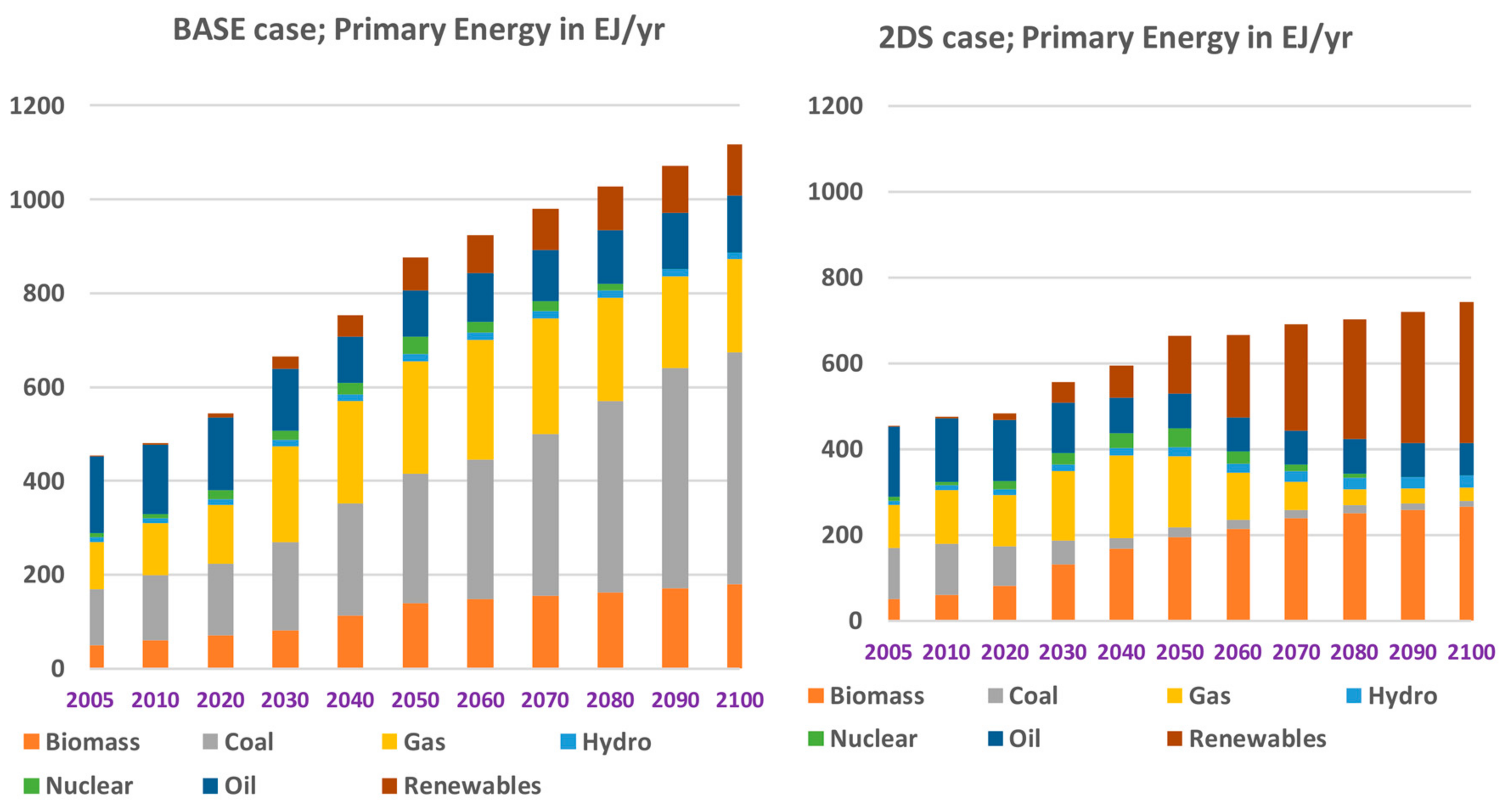
Primary energy consumption (Figure 3) in the BASE case increases from 544 EJ in 2020 to 924 and 1118 EJ/year by 2060 and 2100, respectively. Significant also is the reduction of Primary energy in the 2DS case, which attains levels of around 483, 665, and 743 EJ/year for the same periods. Most important is the fuel substitution that takes place in the 2DS case, where the carbon constraint shifts production to renewables, biomass, and nuclear while it limits the use of oil and gas.

4.3. Electricity Generation

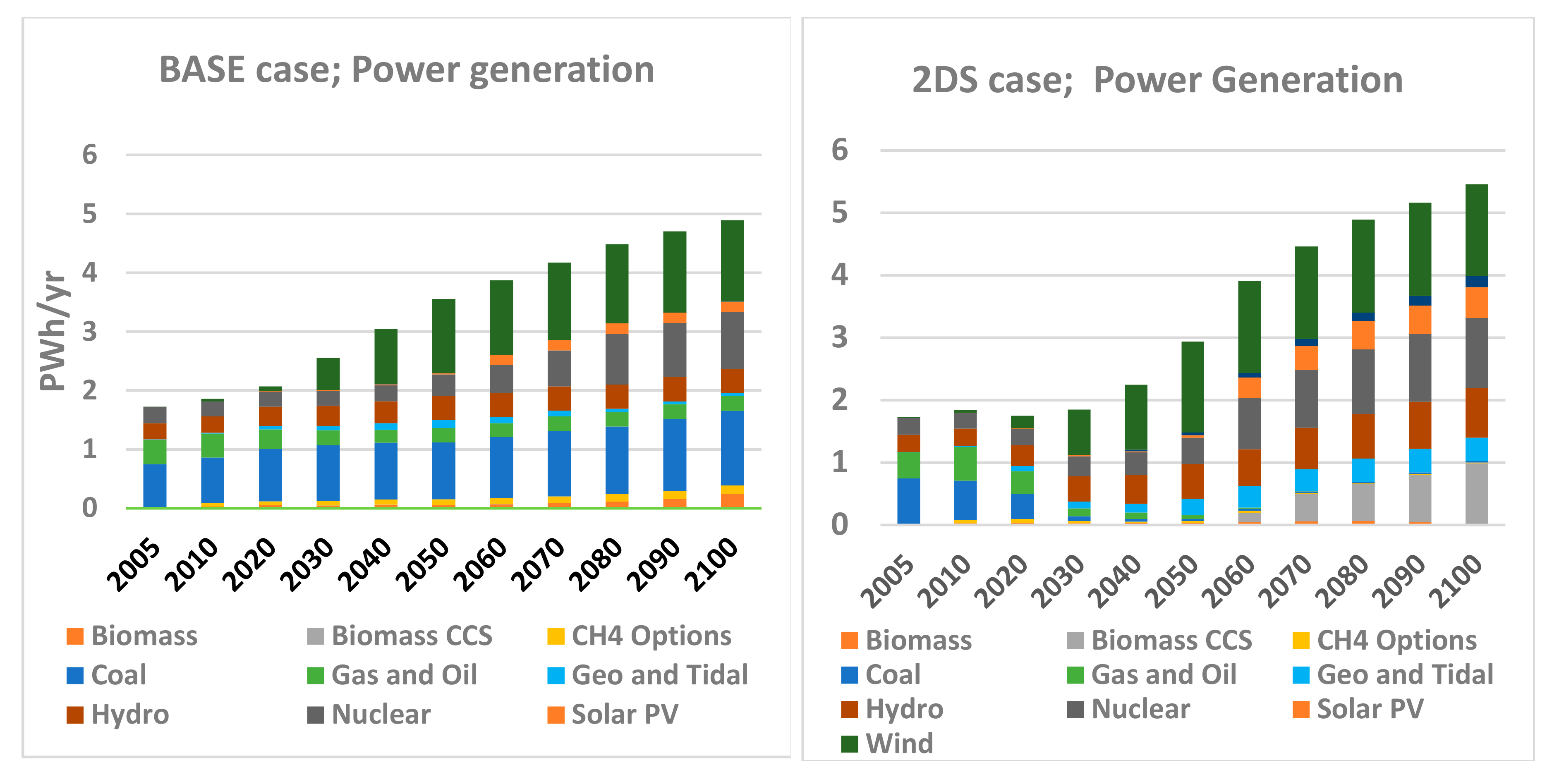
The carbon budget switches power generation technologies towards carbon-free systems, such as renewables (wind and solar), biomass, and nuclear (Figure 4). Due to the limited biomass resources, the use of BECCS technology for power generation is restricted to less than 8 PWh/year while the rest of the biomass is used for the production of biofuels. Interesting is that in the second half of the century (i.e., after 2060), the 2DS electricity generation is above the levels of the BASE case as the stringency of the carbon constraint forces electricity to substitute for fossil fuels in the end-use markets.

4.4. LAP Emissions

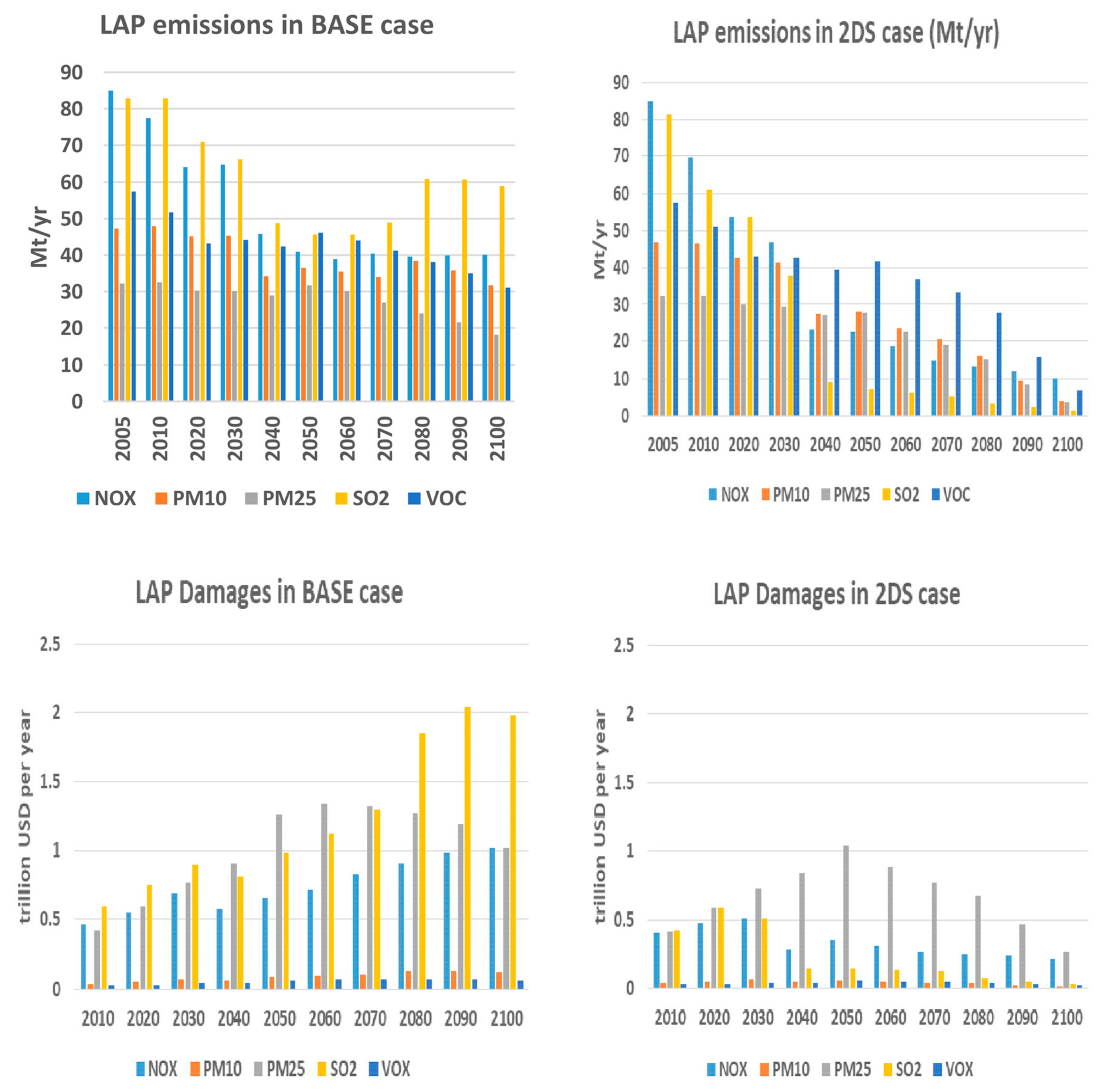
LAP emissions of the BASE case are successfully reduced under the carbon 2DS policy as shown in the upper part of Figure 5. Multiplying ex-post emissions balances with the specific cost per unit of pollutant, we estimate the damages per pollutant and region for the BASE and 2DS cases. The reduction of damages in the 2DS case, relative to the BASE case, defines the secondary benefits of the 2DS policy (Figure 5, below). While in the BASE case damages are dominated by SO₂ and PM2.5 emissions, the 2DS case indicates that PM2.5 is the most significant source of damages.

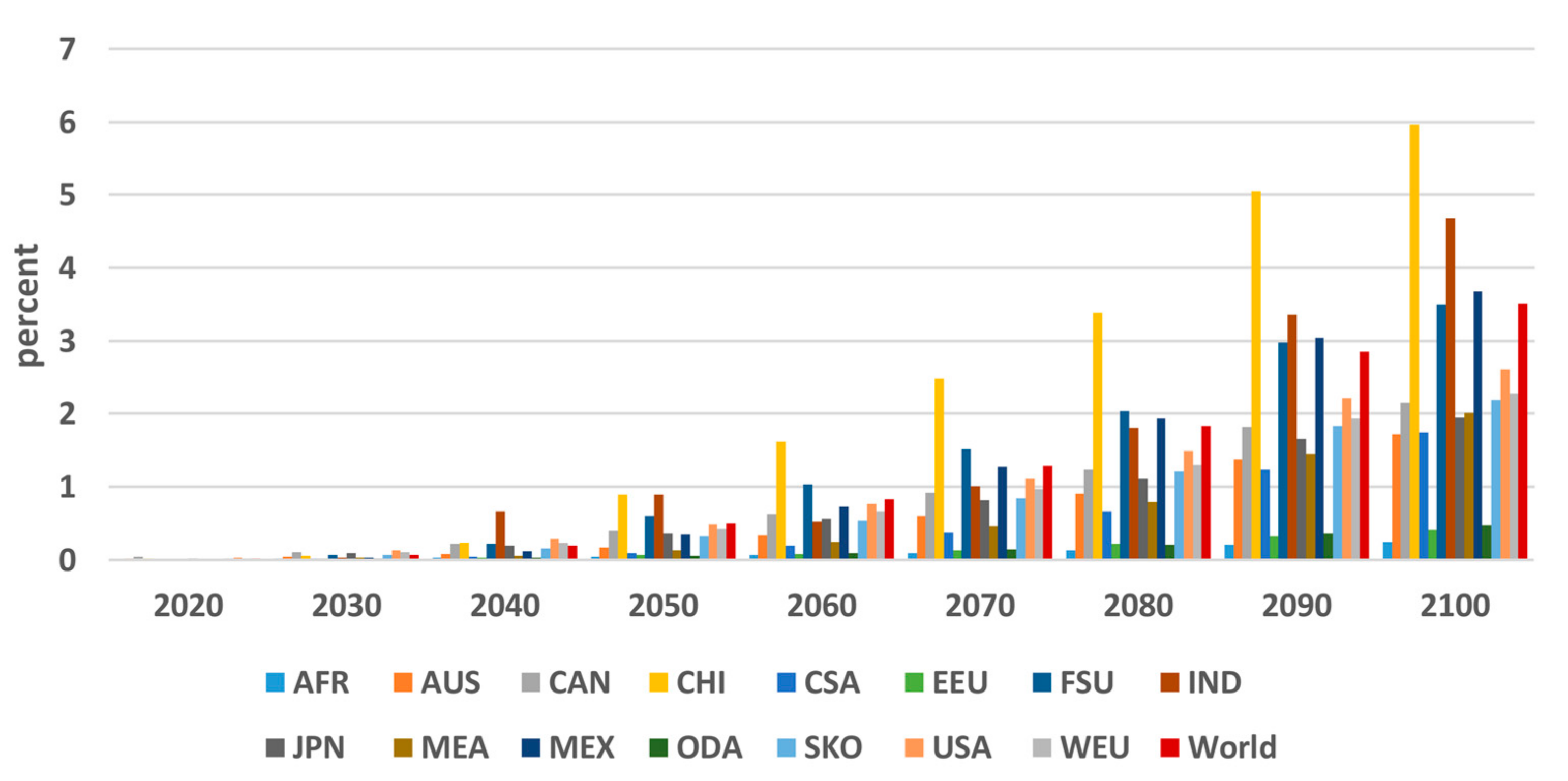
Furthermore, there are primary benefits due to the reduction of market and non-market damages of climate change. These damages can be identified ex-post based on the same relations that define damages in MERGE. For MERGE, market damages are proportional to temperature change while non-market damages depend on the willingness-to-pay to mitigate climate change and are quadratic (or even higher) to post-industrial temperature change. This ex-post assessment of benefits is an alternative evaluation of a Cost and Benefit Analysis (CBA) for the imposed carbon quotas (but not a formal CBA that takes into account damages directly in the utility function of the model). Such formal CBA analysis is technically feasible with TIAM-MACRO, but the equilibrium emissions are expected to be far above those required for the 2DS scenario. The 2DS policy case reduces the risk of climate change associated with the reference development scenario, such as temperature change, sea level rise, and biodiversity. Putting together the cumulated primary and secondary benefits, we obtain the regional, global, and time-dependent development of benefits (Figure 6). In addition, the cumulative undiscounted net benefits (of the 2DS policy) are 1.97% of the cumulative GDP of the BASE case while the relative GDP losses of the mitigation policy are 5.15%. These benefits correspond by 1.04% to the primary benefits of climate policy and by 0.93% to ancillary co-benefits. As shown in Figure 7, China, India, Mexico, and the Former Soviet Union (FSU) benefit above the global average. This is due to the size of the countries and their high emissions in the BASE case.

5. Burden Sharing (BS)

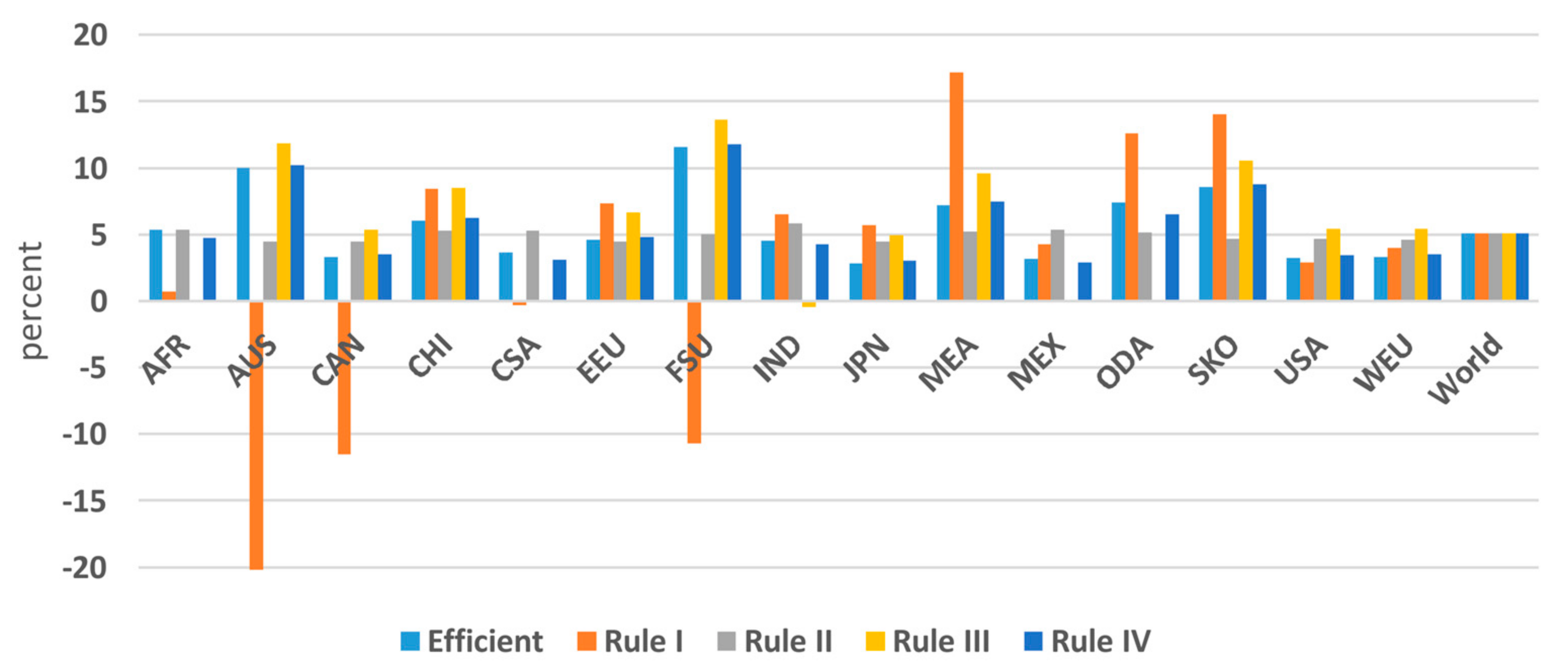
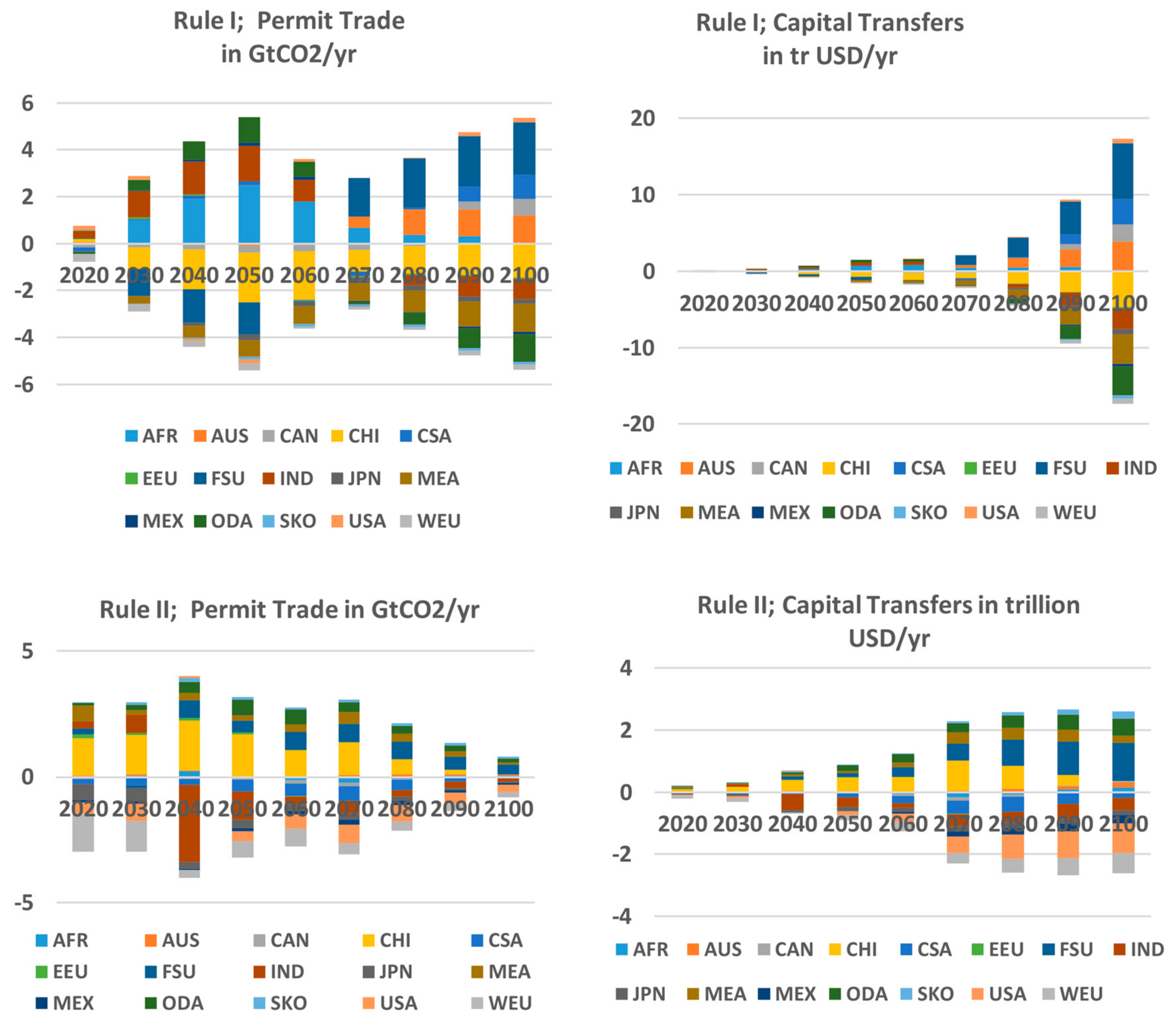
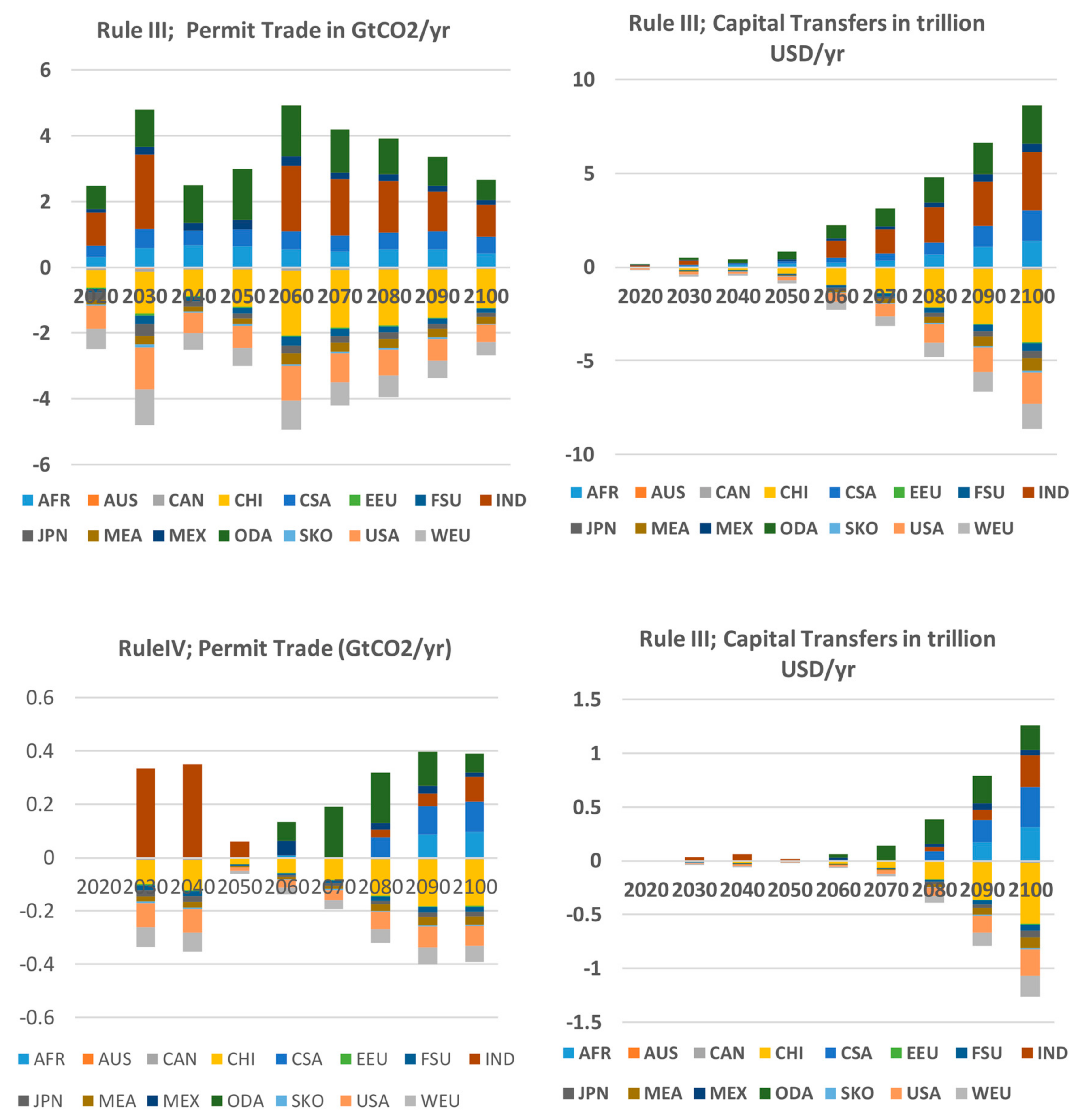
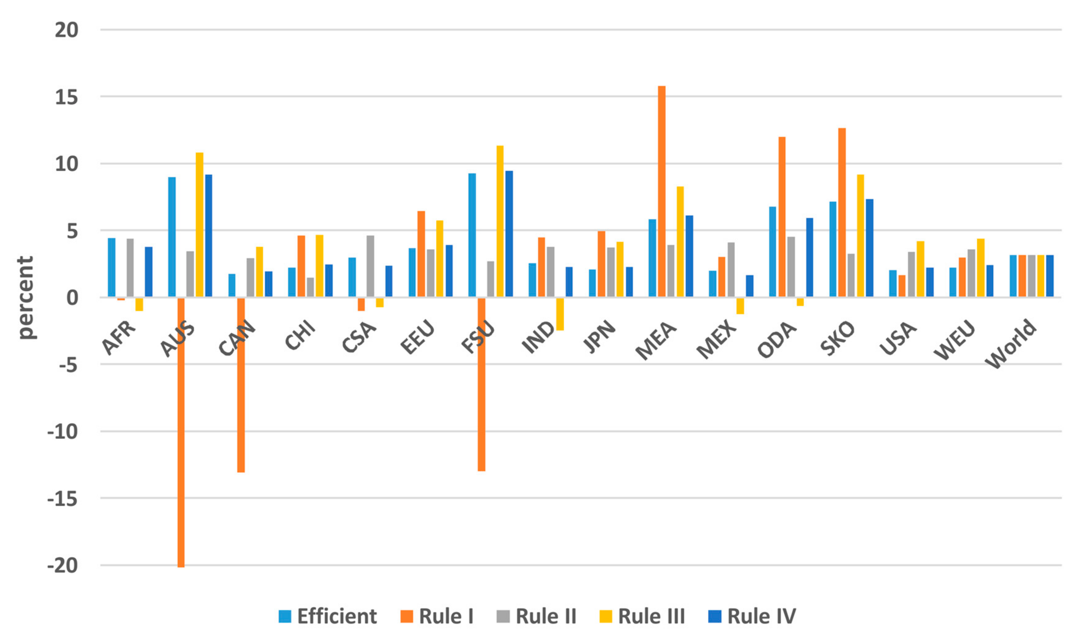
Burden sharing is a market-based mechanism to establish equity, as less-developed countries (LDCs) are not able to finance the transition to a carbon-free economy. However, a distribution of the initial endowment of their emission permits based on equity principles (rules) allows them to trade their emission surpluses and profit from trade. While the average global and undiscounted GDP loss is in the range of 5.15% cumulatively over the model horizon, there is considerable disparity in regional GDP losses in the least cost-efficient solution (Figure 7). For the Efficient solution, United States of America (USA), Japan (JPN), Canada (CAN), and Western Europe (WEU) have cumulative GDP losses of 2.9–3.3%, whereas the Former Soviet Union (FSU), China (CHI), Other Developing Asian Countries (ODA), India (IND), and Africa (AFR) have cumulative GDP losses between 3.7 and 11.6%. Figure 8 explains in detail the trade of permits across regions and the capital transfers for each rule. Rule I assumes equal emissions per capita (egalitarian) in 2050 after a period between 2020 and 2050 where a grandfathering rule applies. Regions such as Australia (highest profit), Canada, and the Former Soviet Union with a large biomass and renewable energy potential stand to gain significantly from this rule. The Middle East energy export countries suffer the largest economic losses relative to the Baseline as the world economy is decarbonized. In the long term, most of the emerging economies have GDP loss that is less in the efficient scenario as opposed to the equal emissions per capita scenario. China, Developing Asia, and India are seen to have unexpected larger economic losses as a result of high growth starting from a low economic level of high carbon intensity. Central and South America and Africa reduce their losses to above or near zero as a result of having slower growth than their emerging economy counterparts.

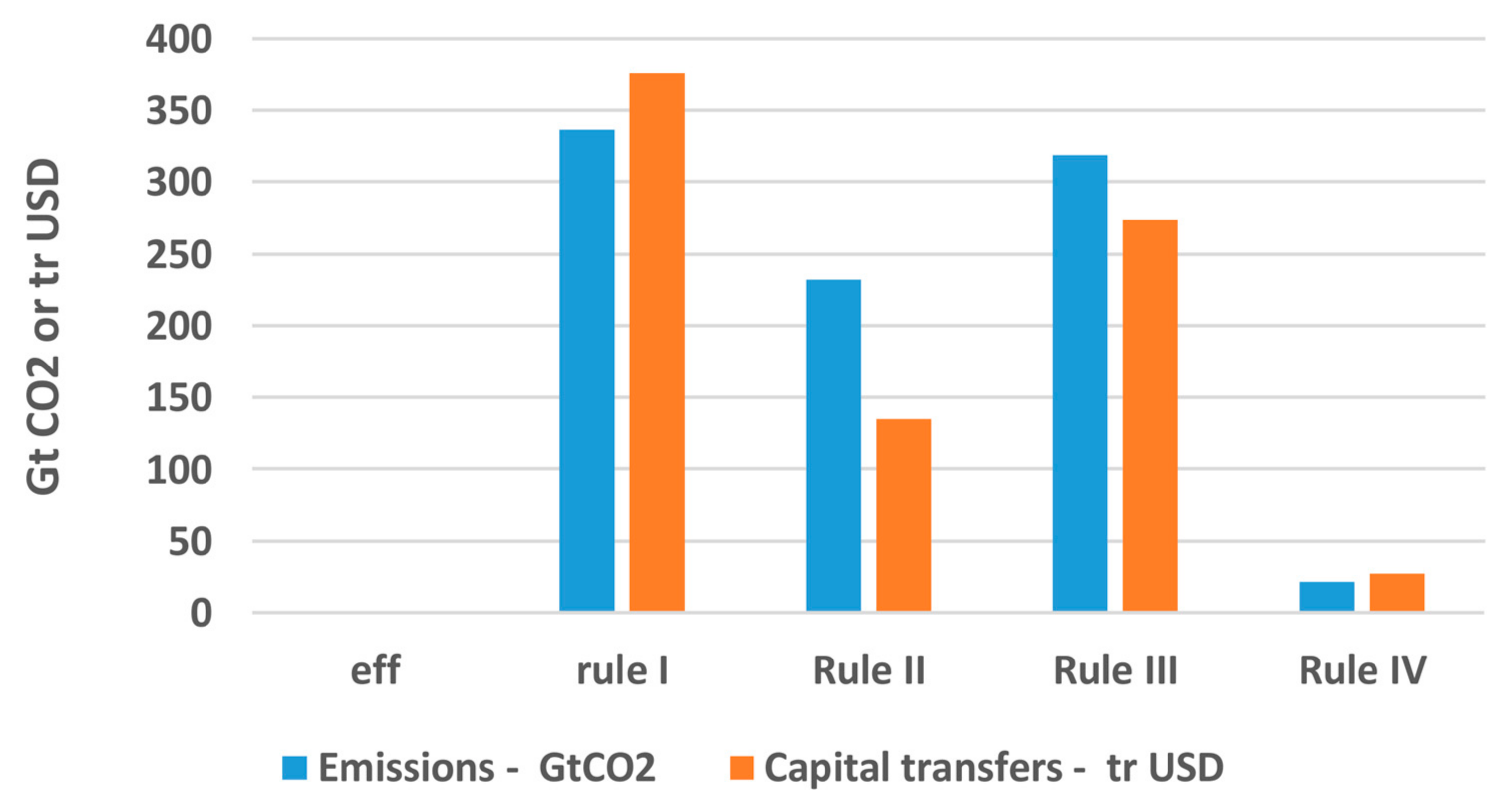
Rules II to IV equalize GDP losses across all regions, compensate LDCs (AFR = Africa, CSA = Central and South America, IND = India, MEX = Mexico, and ODA = Other Developing Asian Countries) for GDP losses or fully compensate the same set of LDCs for their energy cost losses. The redistribution of losses by rule is given in Figure 7. The Burden Sharing rule, which requires the least amount of capital transfers, is the one compensating LDCs for energy cost increases. High income countries, by definition, see GDP losses rise in Rules III and IV, while LDC countries see their GDP losses drop to between 6.5% and 0% over the horizon. Each burden sharing rule presents different winners and losers. Regions that may benefit in the short term do not necessarily gain in the long term nor cumulatively over the model horizon to 2100. This observation points out the difficulties in reaching an agreement, as each region is in favor of the rule that maximizes their profit.

Figure 9 presents the integrals of capital transfers shown on the right-hand side (RHS) of Figure 8 for the different BS rules and the integrals of traded CO₂ emissions on the left-hand side (LHS) of Figure 8. Notice also that the world GDP in 2100 is 314 trillion USD and the world CO₂ emissions for the BASE case are 64.2 GtCO₂ while the GDP integral from 2020 to 2100 is 14,272 trillion USD and the CO₂ emissions 3785 GtCO₂.

Rule IV with the lowest capital transfer requirements compensates LDCs for their extra energy systems costs to decarbonize their economy. Such a compromise has the chance to be accepted as it consists of a win-win situation for both parts. Actually, the transfers required for this rule are so low that one should think about and discuss a technology transfer protocol where the industrialized regions fully undertake the financing of investment for a technology switch towards a decarbonized economy.

6. BS Net of Global Climate Change (GCC) Damages and LAP Externalities

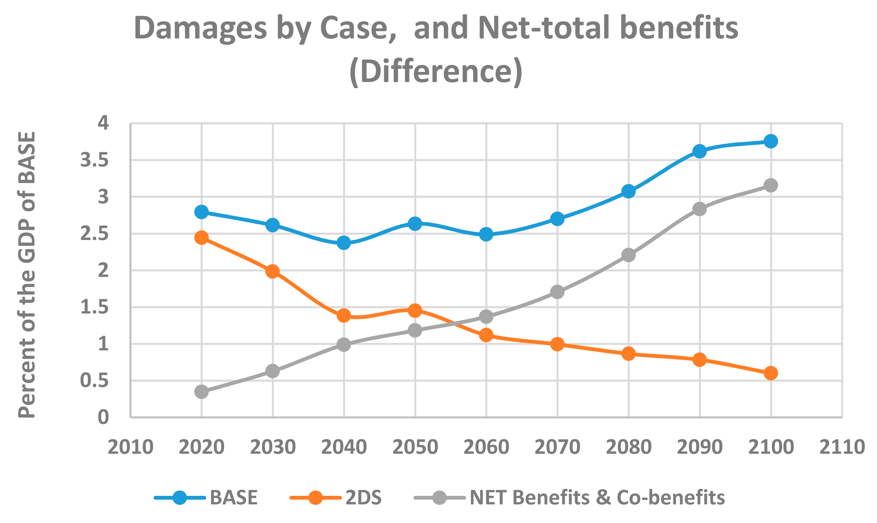
Finally, we proceed to defining the GDP losses net of benefits of climate change mitigation and net of co-benefits due to the reduction of LAP externalities. Figure 10 quantifies the difference of the percentage damages of the 2DS case and the BASE case, which defines the overall net-benefit of the 2DS policy. The BASE case and 2DS start almost at the same level of damages in 2020 as the CO₂ policy constraint is imposed from 2020 onwards. The 2DS damages are at a minimum at the end of the time horizon as temperature is implicitly constrained and simultaneously LAP damages become low. Damages in 2020 are dictated by LAP externalities with climate damages being not yet significant. Taking into consideration the regional representation of the overall net-benefits by region and time, (Figure 6) we estimate the undiscounted world GDP losses (relative to the GDP integral of the BASE case) to be reduced from 5.14% to 3.18% (Figure 11). However, the benefits are again less than the control cost for the 2DS case.

Figure 11 re-defines the regional and global GDP losses relative to the BASE case for the efficient solution, the different BS rules, net of benefits and co-benefits, indicating a significant but partial GDP reduction in losses. This will also reduce the required capital transfers across regions for compensating LDCs.

7. Conclusions

The scope of the article was to demonstrate the analytical capabilities of TIAM-MACRO with some basic examples discussing issues related to climate change. Therefore, we have analyzed the reference development and a case that corresponds to 2 degrees of maximum global warming above pre-industrial levels. The search for an efficient 2 °C scenario is elaborated by imposing appropriate cumulative global CO₂ quotas from 2020 to 2100. We have completed a Second Best analysis, not a Cost Benefit one, but we have evaluated ex-post benefits, such as the reduction of expected climate damages and the expected benefits of improved ambient air quality. Then, we applied burden sharing rules and capital transfers aiming to present arguments that might convince LDCs to participate in a global commitment (potential extension of the present NDCs pledges).

The main methodological achievement of the modelling work carried out for the ETSAP project is the development of a global integrated framework of 15 regional energy system models reflecting all of the details in the energy systems’ restructuring under a climate change constraint. Moreover, based on this model, we perform a ‘full cost’ analysis of the global energy system demonstrating the possibilities of such a tool in evaluating a few key socio-economic-energy-environment scenarios. This integrated framework provides an important platform for future refinements and enhancements of full-cost analyses. However, there is an enormous uncertainty associated with the climate change issue that requires probabilistic risk assessment methods (or stochastic analysis) to complete the picture of climate change assessment. Such studies are technically feasible with the present stage of development of the TIAM family of models, especially when using new high-performance computers with about 100 processors. We also propose a soft link with a model such as GLOBIOM to integrate aspects of land use, land-use change, biomass, food and water uses, and the specification of biomass potential for BECCS, taking into consideration the competition for food production. Another recent model enhancement in TIMES is addressing the extended use of stochastic electricity supply options based on renewables related to de-carbonization policies together with constraints representing enhanced storage options, load management, and the grid topology in Switzerland [27].

The main policy conclusions based on TIAM-MACRO evaluations are as follows:

• The 2 °C policy is technically feasible and accepting burden sharing redistribution rules can be equitable. However, total cumulative (2020–2100) and undiscounted GDP losses are high (5.15% compared to the GDP integral of the BASE case). This cost is within the economy and the energy system exclusive of the side benefits, i.e., it is an economically efficient second best solution.
• However, the pre-conditions of technical feasibility for the 2DS case are related to the assumptions underlying the calculations, such as a universal determination of industrialized nations to proceed first with their own commitments, second with assisting LDCs to materialize the transition of their energy systems, and finally with increasing Research & Development & Demonstration (R&D&D) spending of public and private resources for the development of advanced technology, such as BECCS, and for supporting related infrastructures.
• The climate policy brings also ancillary benefits that reduce damage from local pollutants (SO₂, NOx, PM, VOC) by exploiting synergies. Carbon mitigation policies reduce global climate change damages and improve ambient air quality; therefore, they compensate for part of the cost of mitigating climate change.
• The analysis quantifies the avoided climate damages and the co-benefits of LAP control always under the reservation of uncertainties in the climate science, in the ambient air quality and damages, and in the economics of climate change. Both benefits result in a net benefit of about two percentage points (p. p.) of the BASE case’s GDP integral. Nevertheless, the mitigation cost of climate change for the 2DS policy case is not fully balanced and remains higher than the benefits by three percentage points.
• These benefits address part of all of the potential benefits of climate policies. Co-benefits in TIAM do not account for indoor pollution and ecosystem services nor for natural capital conserved via climate mitigation policy. We do not consider also the improvement of air quality as a consequence of climate change control that could significantly reduce health impacts [16].
• The consideration of burden sharing between regions defines equitable scenarios. Equal relative GDP losses is a balanced burden sharing allocation rule but is less appropriate for LDCs. The full compensation of the energy system cost increase requires low capital transfers to LDCs for their investments in favor of a carbon-free technology switch. The capital transfers of Rule IV in favor of LDCs are low and therefore one could argue to fully support investments via technology transfer protocols towards a decarbonized economy.

References

1. Chiodi, A.; Donnellan, T.; Breen, J.; Deane, P.; Hanrahan, K.; Gargiulo, M.; Ó Gallachóir, B.P. Integrating agriculture and energy to assess GHG emissions reduction: A methodological approach. Clim. Policy 2015, 16, 215–236. [Google Scholar] [CrossRef]
2. Fricko, O.; Havlik, P.; Rogelj, J.; Klimont, Z.; Gusti, M.; Johnson, N.; Ermolieva, T. The marker quantification of the Shared Socioeconomic Pathway 2: A middle-of-the-road scenario for the 21st century. Glob. Environ. Chang. 2017, 42, 251–267. [Google Scholar] [CrossRef] [Green Version]
3. Kriegler, E.; Bauer, N.; Popp, A.; Humpenöder, F.; Leimbach, M.; Strefler, J.; Mouratiadou, I. Fossil-fueled development (SSP5): An energy and resource intensive scenario for the 21st century. Glob. Environ. Chang. 2017, 42, 297–315. [Google Scholar] [CrossRef]
4. Emmerling, J.; Drouet, L.; Reis, L.A.; Bevione, M.; Berger, L.; Bosetti, V.; Malpede, M. The WITCH 2016 Model-Documentation and Implementation of the Shared Socioeconomic Pathways. FEEM Working Paper 42. 2016. Available online: http://www.feem.it/getpage.aspx?id=8521 (accessed on 11 April 2018).
5. Kypreos, S.; Lehtilä, A. Decomposing TIAM-MACRO to Assess Climatic Change Mitigation. Environ. Model. Assess. 2015, 20, 1–11. [Google Scholar] [CrossRef]
6. International Energy Agency (IEA). Energy Technology Perspectives-Scenarios & Strategies to 2050; International Energy Agency: Paris, France, 2006. [Google Scholar]
7. US-EIA. Energy Outlook; International Energy Agency: Paris, France, 2007. [Google Scholar]
8. Howells, M.; Rogner, H.; Strachan, N.; Heaps, C.; Huntington, H.; Kypreos, S.; Roehrl, A. OSeMOSYS: The Open Source Energy Modeling System: An introduction to its ethos, structure and development. Energy Policy 2011, 39, 5850–5870. [Google Scholar] [CrossRef]
9. PRIMES. 2016. Available online: www.e3mlab.ntua.gr (accessed on 11 April 2018).
10. IEA Statistics. Available online: https://www.iea.org/statistics/ (accessed on 11 March 2018).
11. IEA/ETSAP Project. Available online: https://iea-etsap.org/ (accessed on 8 March 2018).
12. Loulou, R.; Labriet, M. ETSAP-TIAM: The TIMES integrated assessment model Part I: Model structure. Comput. Manag. Sci. 2008, 5, 7–40. [Google Scholar] [CrossRef]
13. Loulou, R. ETSAP-TIAM: The TIMES integrated assessment model, part II: Mathematical formulation. Comput. Manag. Sci. 2008, 5, 41–66. [Google Scholar] [CrossRef]
14. IEA-WEO. Special Issue on Energy and Air Pollution; International Energy Agency: Paris, France, 2016. [Google Scholar]
15. Kitous, A.; Keramidas, K.; Vandyck, T.; Saveyn, B.; Van Dingenen, R.; Spadaro, J.; Holland, M. Global Energy and Climate Outlook 2017: How Climate Policies Improve Air Quality; JRC107944, EUR 28798 EN; European Commission, Joint Research Centre: Seville, Spain, 2017; pp. 71–72. [Google Scholar]
16. Garcia-Menendez, F.; Saari, R.K.; Monier, E.; Selin, N.E. US Air Quality and Health Benefits from Avoided Climate Change under Greenhouse Gas Mitigation. Environ. Sci. Technol. 2015, 49, 7580–7588. [Google Scholar] [CrossRef] [PubMed]
17. Volkart, Integration of Energy-Economic System Modelling and Multi-Criteria Analysis. Ph.D. Thesis, ETH Zurich/Paul Scherrer Institute, Switzerland, Europe, 2016.
18. NEEDS. New Energy Externalities Developments for Sustainability. 2009. Available online: http://www.needs-project.org (accessed on 11 April 2018).
19. EMEP/EEA. Air Pollutant Emission Inventory Guidebook. 2013. Available online: https://www.eea.europa.eu/themes/air/emep-eea-air-pollutant-emission-inventory-guidebook (accessed on 11 April 2018).
20. EDGAR. Emission Database for Global Atmospheric Research (EDGAR) for the Year 2005. Available online: http://edgar.jrc.ec.europa.eu/overview.php?v=42 (accessed on 11 April 2018).
21. Shay, C.; DeCarolis, J.; Loughlin, D.; Gage, C.; Yeh, S.; Vijay, S.; Wright, E.L. EPA U.S. National MARKAL Database: Database Documentation; EPA-600/R-06/057; Environmental Protection Agency: Washington, DC, USA, 2006.
22. Manne, A.; Mendelsohn, R.; Richels, R. MERGE: A model for evaluating regional and global effects of GHG reduction policies. Energy Policy 1995, 23, 17–34. [Google Scholar] [CrossRef]
23. GEM-E3. Manual and Documentation of the GEM-E3 Model. 2016. Available online: https://ec.europa.eu/jrc/en/gem-e3/model (accessed on 11 April 2018).
24. Kriegler, E.; Tavoni, M.; Aboumahboub, T.; Luderer, G.; Calvin, K.; Demaere, G.; Van Vuuren, D.P. What does the 2 °C target imply for a global climate agreement in 2020? The limits study on Durban platform scenarios. Clim. Chang. Econ. 2013, 4, 1340008. [Google Scholar] [CrossRef]
25. Socrates Kypreos: Equitable Burden Sharing: Modelling the Macroeconomic Impacts of the Carbon Constrained Energy System in ETSAP-TIAM-MACRO, International Energy Workshop in Cork, Ireland in 2016. Available online: https://www.ucc.ie/en/iew2016/presentations/ (accessed on 8 March 2018).
26. Tavoni, M.; Kriegler, E.; Riahi, K.; Van Vuuren, D.P.; Aboumahboub, T.; Bowen, A.; Luderer, G. Post-2020 climate agreements in the major economies assessed in the light of global models. Nat. Clim. Chang. 2015, 5, 119–126. [Google Scholar] [CrossRef] [Green Version]
27. ISCHESS—Integration of Stochastic Renewables in the Swiss Electricity Supply System. Available online: https://www.psi.ch/lea/HomeEN/Final-Report-ISCHESS-Project.pdf (accessed on 11 March 2018).
1
Naturally, the methodology followed in TIAM-MACRO for the cost of local pollutants is simple as it is based on emission inventories only. On the contrary, the approach described in [16] follows the causality chain and concludes about the atmospheric quality of each scenario. According to [16], climate change, exclusive of changes in air pollutant emissions, can significantly impact ozone (O3) and fine particulate matter (PM2.5) pollution across the U.S. and increases the associated health effects. Clearly, by excluding such analysis concerning the impacts of climate change to air quality, we underestimate health impacts. Figure 3, page 7585, in [16] indicates that such improved air quality could offset the cost of climate policy by 11–14.5%, which for our case corresponds roughly to another 0.8 p.p. of the estimated climate change mitigation cost.
2
It is quite easy to integrate in TIAM the MACRO Stand-Alone (MSA) module. One has to just include Equations (2)–(11) (excluding Equation (8)) into the set of equations modelling TIAM and to solve the overall model maximizing Equation (2). The result will be a non-linear model with about a million linear equations that is not tractable even with the best available personal computer.
3
The values shown in Figure 2b correspond to an exponential growth factor of 1.6289 = (1.05)10 per decade, induced by the cumulative CO2 constraint, and start from 66 $/tCO2 in 2020. 5% per year is the discount factor applied in TIMES.
Figure 1. Positioning the reference development (BASE) and the 2 °C scenario (2DS) cases within the published emission trajectories. RCP: representative concentration pathways.
Systems 06 00010 g001
Figure 2. (a) Regional emissions for BASE and 2DS scenarios; (b) Undiscounted shadow prices for the 2DS mitigation scenario.
Systems 06 00010 g002
Figure 3. Primary energy production by fuel for the BASE and 2DS cases.
Systems 06 00010 g003
Figure 4. Electricity generation by technology for the BASE and the 2DS cases.
Systems 06 00010 g004
Figure 5. Local atmospheric pollutant (LAP) emissions and damages (external costs) estimated ex-post for the BASE and the 2DS cases. NOX = Nitrogen Oxides; PM = Particulate Matter; VOX = Volatile Organic Compounds.
Systems 06 00010 g005
Figure 6. Annual and regional relative Net Benefits and Co-Benefits of the 2DS case relative to the gross domestic product (GDP) of the BASE case.
Systems 06 00010 g006
Figure 7. Regional cumulative and undiscounted GDP losses (positive) relative to the BASE case, from 2020 to 2100, for the Efficient 2 °C scenario and under different burden sharing (BS) rules.
Systems 06 00010 g007
Figure 8. Equitable Burden Sharing Rules I–IV (top to bottom); Carbon Permits GtCO2 (Left), Undiscounted Capital Transfers in trillions of U.S. Dollars (Right). Rule (I) Egalitarian with equal emissions per capita after 2050, Rule (II) Capital Transfers to Equalize relative regional GDP losses, Rule (III) Full Compensation of GDP Losses for developing countries, Rule (IV) Full Compensation of energy system costs increase for less-developed countries (LDCs).
Systems 06 00010 g008aSystems 06 00010 g008b
Figure 9. World CO2 cumulative emissions trade and the associated undiscounted Capital Transfers for purchasing permits under different BS Rules.
Systems 06 00010 g009
Figure 10. Benefits and co-benefits for the BASE and 2DS cases and the Net Benefits and Co-Benefits of the 2DS case relative to the GDP of the BASE case.
Systems 06 00010 g010
Figure 11. Regional cumulative GDP losses (positive) net of benefits and co-benefits relative to the Base scenario for the Efficient 2 °C scenario and the different BS rules.
Systems 06 00010 g011