
Exploring Intra-Urban Accessibility and Impacts of Pollution Policies with an Agent-Based Simulation Platform: GaMiroD

 , , , and
Abstract
:1. Introduction
2. Modeling and Simulation of Urban Daily Mobility
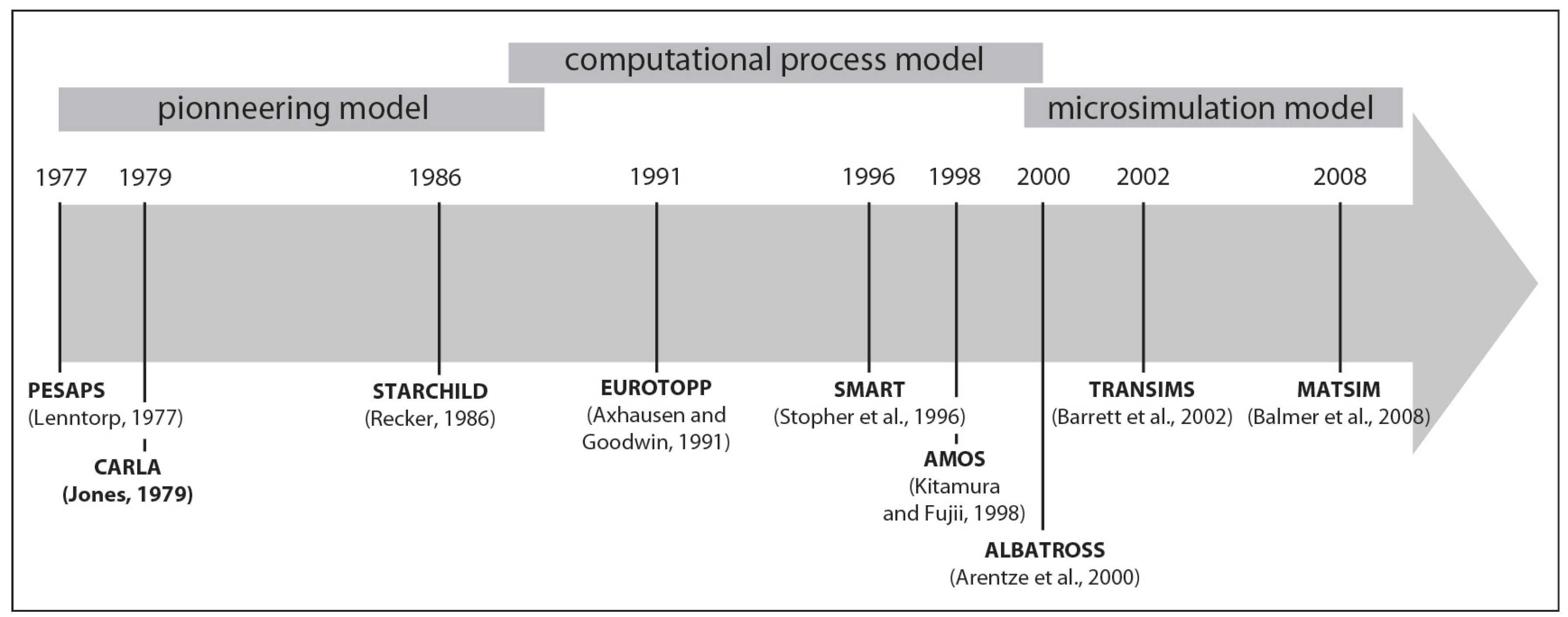
2.1. State of the Art of Activity Based Approach
- No consideration is made of the linked sequence of activities in the course of one trip;
- Movements are not situated in a specific space and/or time;
- The portrayal of behavior is oversimplified. Efficiency is over-emphasized in explaining individual choice of transportation mode, to the detriment of studying many kinds of factors that might influence the choice;
- There is no specification of the relationships between trips, with limitations associated with modes of transportation, or with activity-plans or personal obligations;
- The decision-making process studied in aggregates does not take into account the interactions among individuals and other household members, notably in the context of resource sharing (a car, for example).

- Agent to introduce individual behavior;
- Activity in order to address a schedule and trip;
- Actors to consider policy for forecasting real case studies.
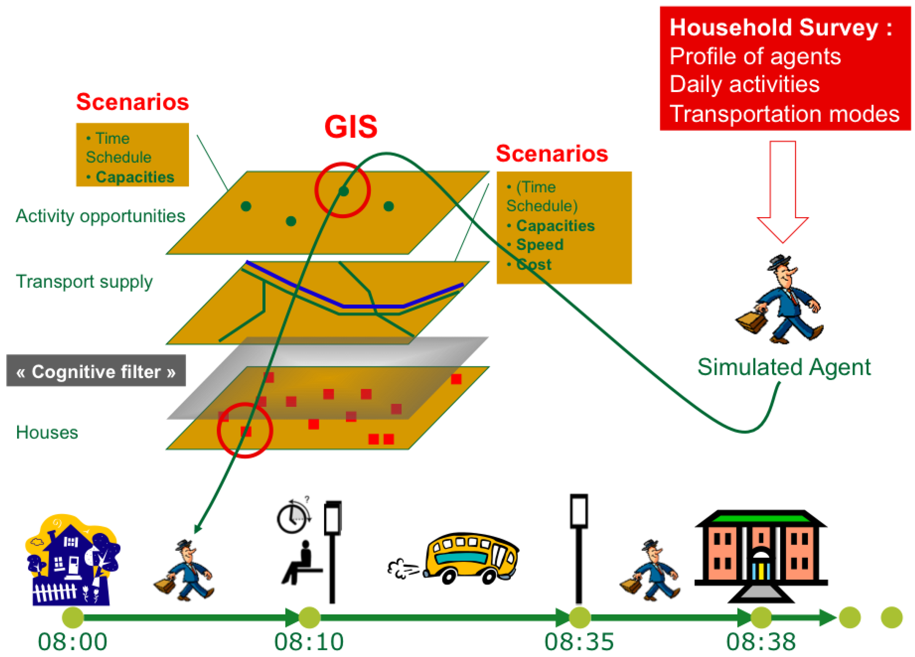
2.2. The MIRO Approach

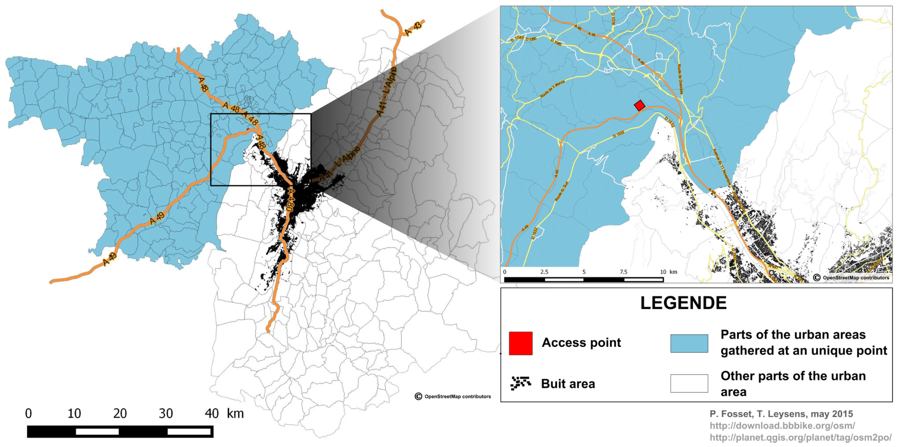
3. Defining a Virtual City
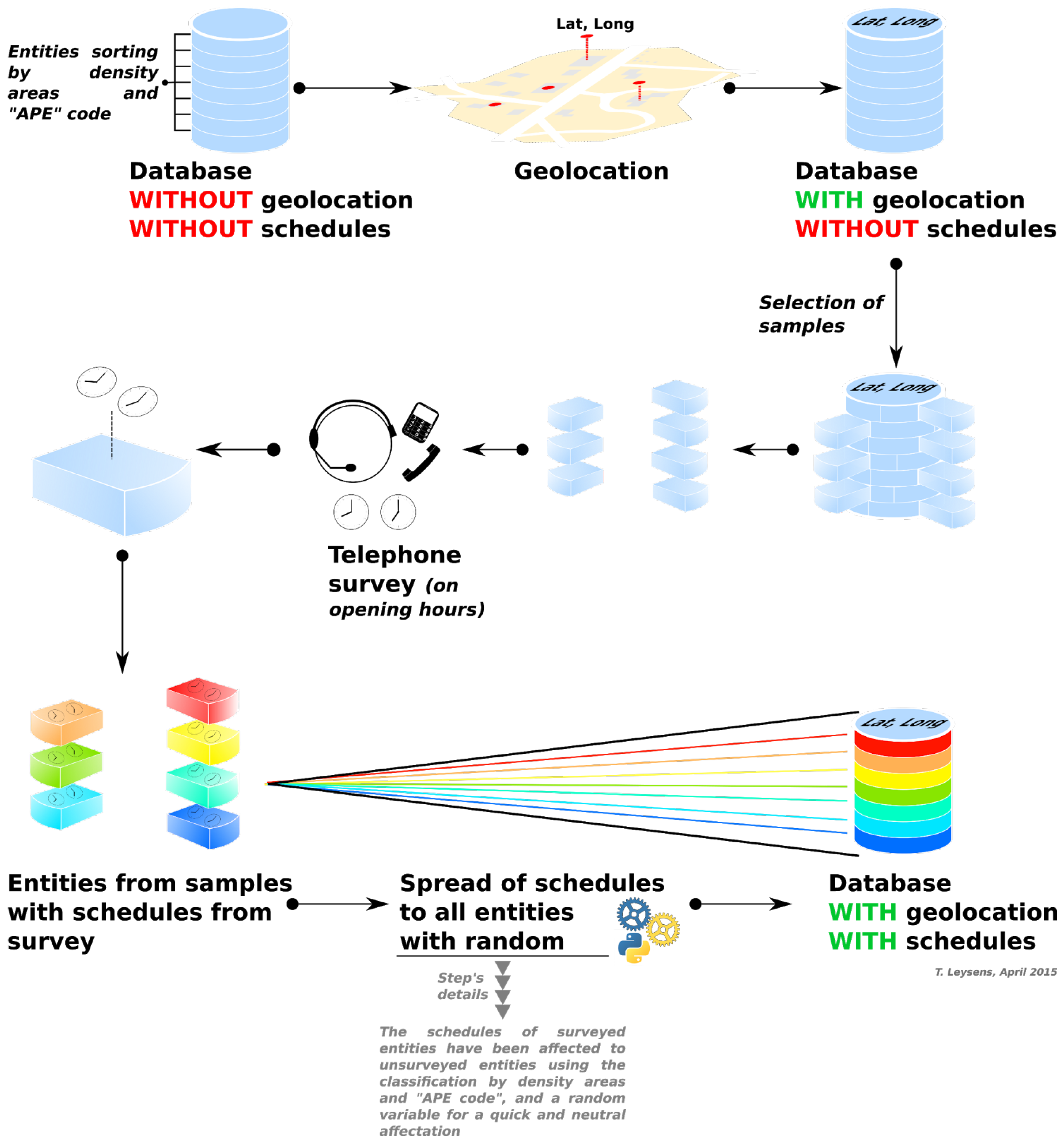
3.1. Constitution of the Spatio-Temporal Database of Opening Hours of Grenoble Urban Resources

3.2. Generating the Synthetic Population
3.2.1. Survey Data as an Input

| Category | Headcount |
|---|---|
| 1: Active people | 3914 |
| 2: Single mothers/Part-time workers | 1313 |
| 3: Unemployed | 577 |
| 4: Active and unemployed 40–64 years old people | 2706 |
| 5: Students | 1283 |
| 6: Retired people | 2131 |
| 7: Young people (going to school) | 2897 |
3.2.2. Data Process and Validation of the Results
| Attribute | Dependencies | Levels |
|---|---|---|
| Category | age | [1,2,3,4,5,6,7] |
| Age | category | 5:17, 18:24, 25:34, 35:49, 50:64, 65:100 |
| Gender | category | man, woman |
| Area | category | One of the 97 area |
| Main Activity | category | Work, Study, Shopping, etc. (8 possibilities) |
| Vehicle type | age, area | No vehicle, authorized vehicle (registred after 2001), un authorized vehicle (registred before 2001) |
| Category | Gender | Frequency |
|---|---|---|
| 0 | 1 | 1992 |
| 1 | 1 | 183 |
| 2 | 1 | 273 |
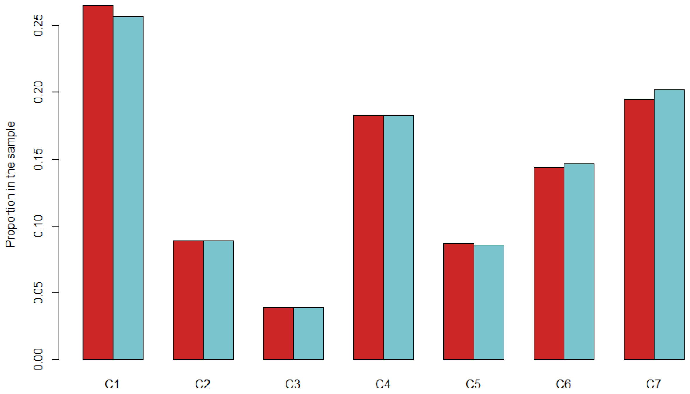
| Attribute | Value | Relative Error |
|---|---|---|
| Category | 0 | 0.007 |
| 1 | 0.012 | |
| 2 | 0.008 | |
| 3 | 0.006 | |
| 4 | 0.016 | |
| 5 | 0.002 | |
| 6 | 0.001 | |
| Gender | Man | 0.001 |
| Woman | 0.001 | |
| Age groups | [5;17] | 0.001 |
| [18;24] | 0.011 | |
| [25;34] | 0.001 | |
| [35;49] | 0.011 | |
| [50;64] | 0.006 | |
| [65+] | 0.002 | |
| Area | [100;199] | 0.002 |
| [200;299] | 0.011 | |
| [300;399] | 0.004 | |
| [400;499] | 0.008 | |
| [500;599] | 0.005 | |
| [600;699] | 0.019 | |
| [700;799] | 0.036 | |
| [800;899] | 0.013 | |
| [900;999] | 0.006 |
3.2.3. Localization of Agents

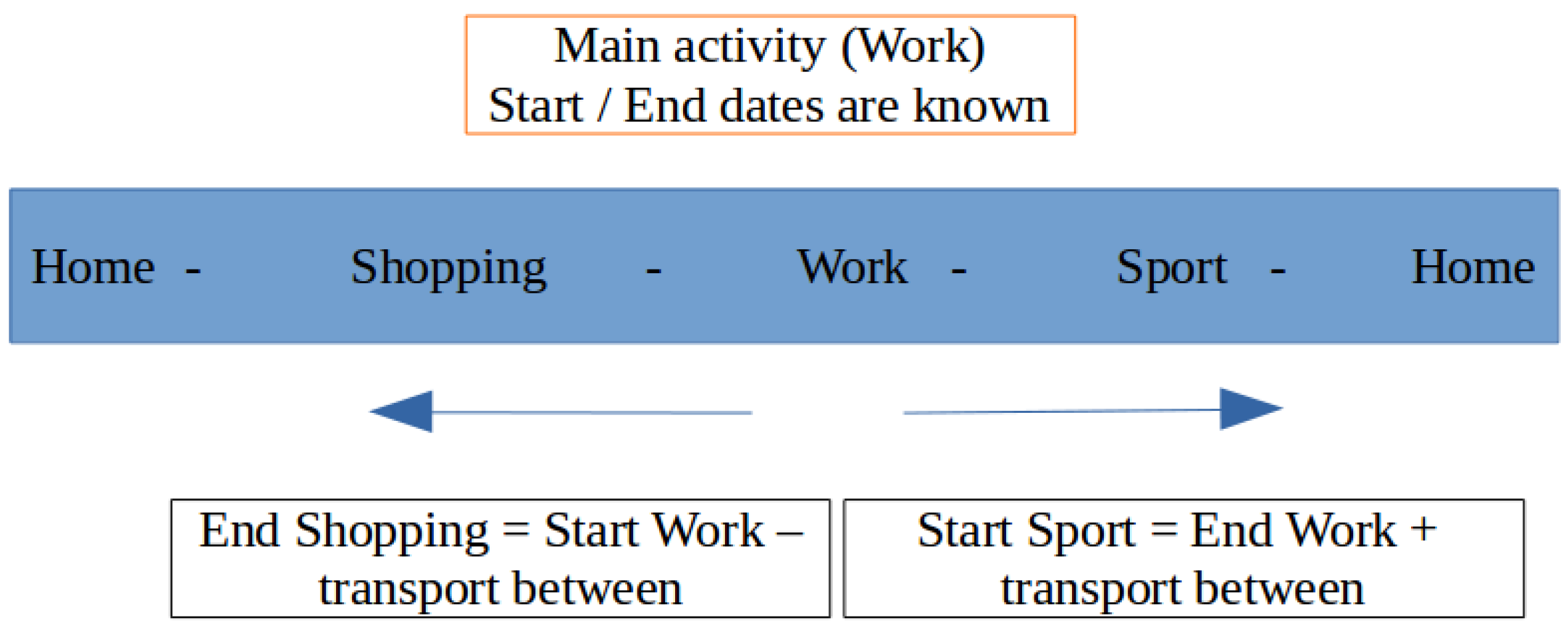
3.2.4. Generation of Agent’s Schedule
| ID_Pers | ID_Schedule | ID_ACT | ACTIVITY | DATE_BEGINNING | DATE_ENDING |
|---|---|---|---|---|---|
| 0 | 0 | 0 | Home | 0 | 49,440 |
| 0 | 0 | 1 | Work | 49,500 | 62,233 |
| 0 | 0 | 2 | Sport | 62,533 | 65,206 |
| 0 | 0 | 3 | Work | 65,326 | 78,059 |
| 0 | 0 | 4 | Home | 78,119 | 86,400 |
| 0 | 0 | 0 | Home | 0 | 29,091 |
| 0 | 0 | 1 | Study | 29,151 | 33,701 |
| 0 | 0 | 2 | Work | 33,881 | 60,751 |
| 0 | 0 | 3 | Study | 60,931 | 74,579 |
| 0 | 0 | 4 | Home | 74,369 | 86,400 |
3.2.5. Utility Function and Decision Process
| Active People | Single Mothers/Part-Time Workers | Unemployed | Active and Unemployed 50–64 Years Old People | Students | Retired People | Young People (Going to School) | |
|---|---|---|---|---|---|---|---|
| Working time | 0.584*** | 0.358*** | 0.312*** | 0.152*** | |||
| Travel time to work | |||||||
| Study time | 0.118*** | 0.135*** | |||||
| Travel time to place of study | −0.124*** | −0.166*** | |||||
| Purshasing time | 1.36** | 5.12*** | 2.18*** | 0.236*** | 2.26** | ||
| Travel time to purshase | −0.242*** | −0.257*** | −0.286*** | −0.127*** | |||
| Health time | 0.811*** | 0.5*** | |||||
| Travel time to health facilities | −0.167*** | −0.268*** | |||||
| Administrative procedures time | 0.307*** | ||||||
| Travel time to administrative procedures | −0.303*** | ||||||
| Leisure time | 1.77*** | 2.0*** | 3.16*** | 6.18*** | 0.313*** | 2.13*** | 0.39*** |
| Travel time to leisure activity | |||||||
| Accompanying time | 2.58*** | 4.0*** | 4.48*** | 0.25* | |||
| Lunch time | −0.191*** | 0.231*** | |||||
| Travel time to lunch | −0.078 | −0.087 |
4. The GaMiroD Model
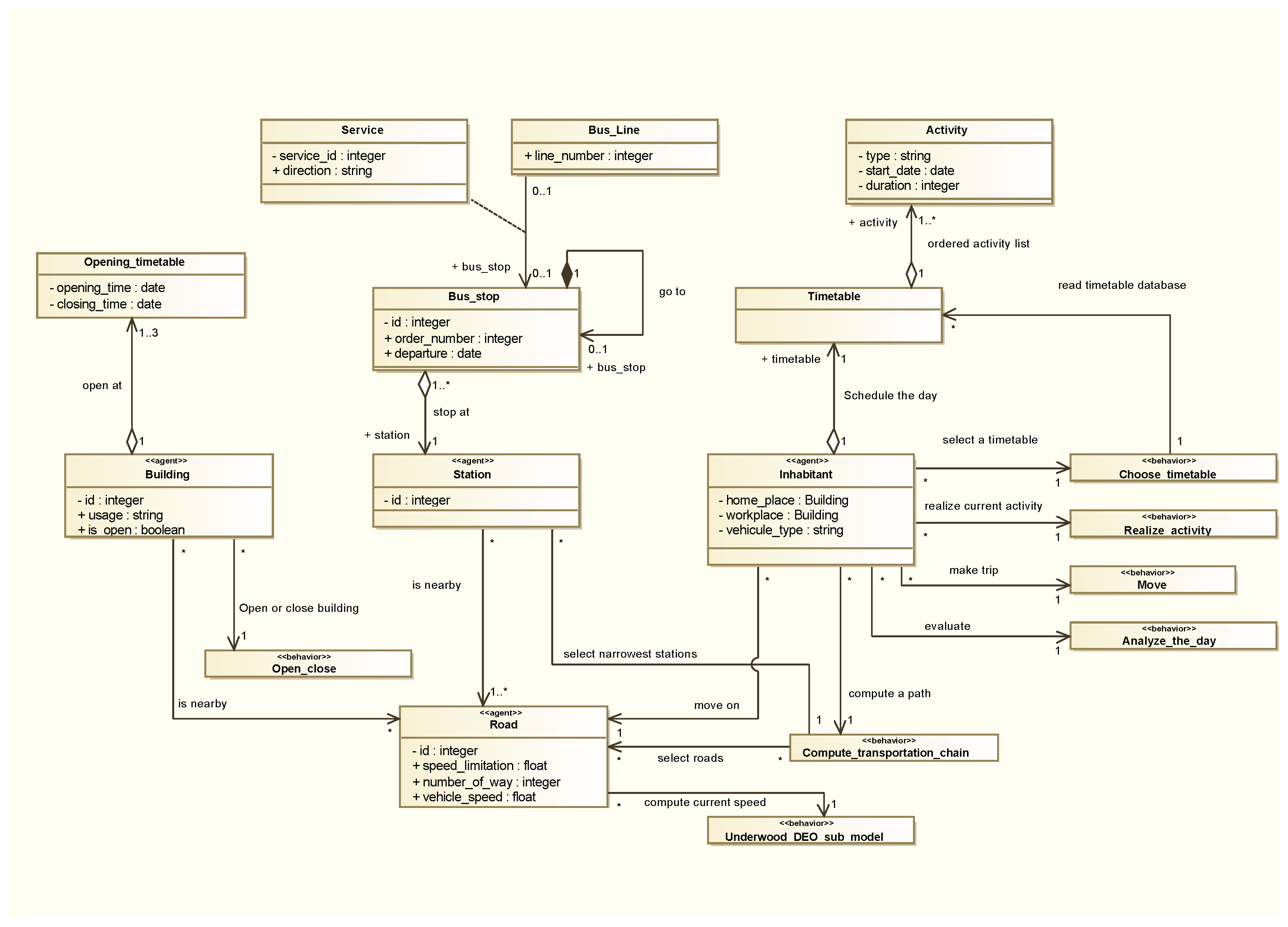
4.1. Model Composition
- “Inhabitants” represent people living in the city and moving along the day to achieve their scheduled activities. The population of “inhabitant” agents is initialized following the synthetic population generation process described in previous sections.
- “Buildings” (~70,000 elements) are generated as agents from a shape file, identifying for each building in Grenoble the main associated services with their opening and closing times.
- “Stations” corresponds to the whole set of bus stations (750 in Grenoble), defined as agents holding informations regarding bus lines and their time schedules.
- “Roads” agents (~80,000) are defined by their capacity, speed limitation, and number of lanes. They are organised as a street network from which travelling paths can be computed.
4.2. Design Model
4.2.1. A Descriptive Multi-Agent-System Based on Data
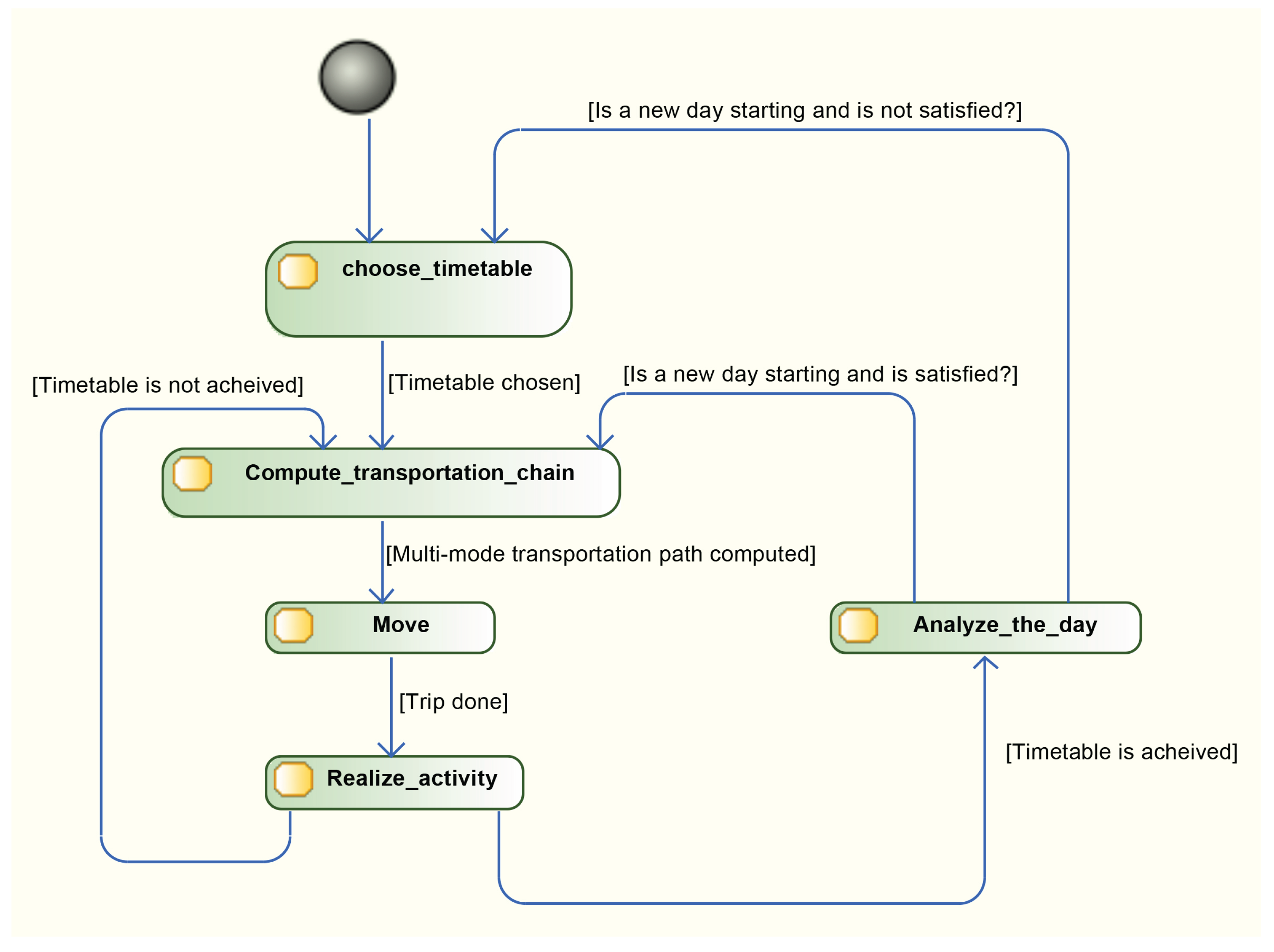
4.2.2. A Highly Dynamic Multi-Agent System
- “choose_timetable” Ten timetable are associated to inhabitant during the population generation. One of them is selected according to agent state and utility function;
- “compute_transportation_chain” Before moving, each agent computes and chooses (based on the time estimation from the Dijkstra shortest path algorithm) its trip from its current location to the next activity location. Multi-modal chains are allowed, for example 3 km by car to go to the bus station, then 2 km by bus to another station and finally 500 m walking to the destination. Transportation mode choice depends on social characteristics of agents, and particularly whether they possess a car or not;
- “move” Realize the journey between two activities according to the transportation chain computed in the previous task;
- “realize_activity” Realize an activity until it is finished;
- “analyze_the_day” The timetable is achieved. Agents analyze their performance of the day and compute a satisfaction rate. They keep their current timetable if it is acceptable or select a new one if needed.
4.2.3. A Macroscopic Traffic Model Applied at a Microscopic Level
- the speed of vehicles driving on edge i;
- the free-flow speed (speed limitation) of edge i;
- the maximum traffic capacity of edge i, that takes into account the number of lanes and the length;
- the number of vehicles driving of edge i, and
- α a congestion impact factor.
4.2.4. The Particulate Matter (PM10) Emission
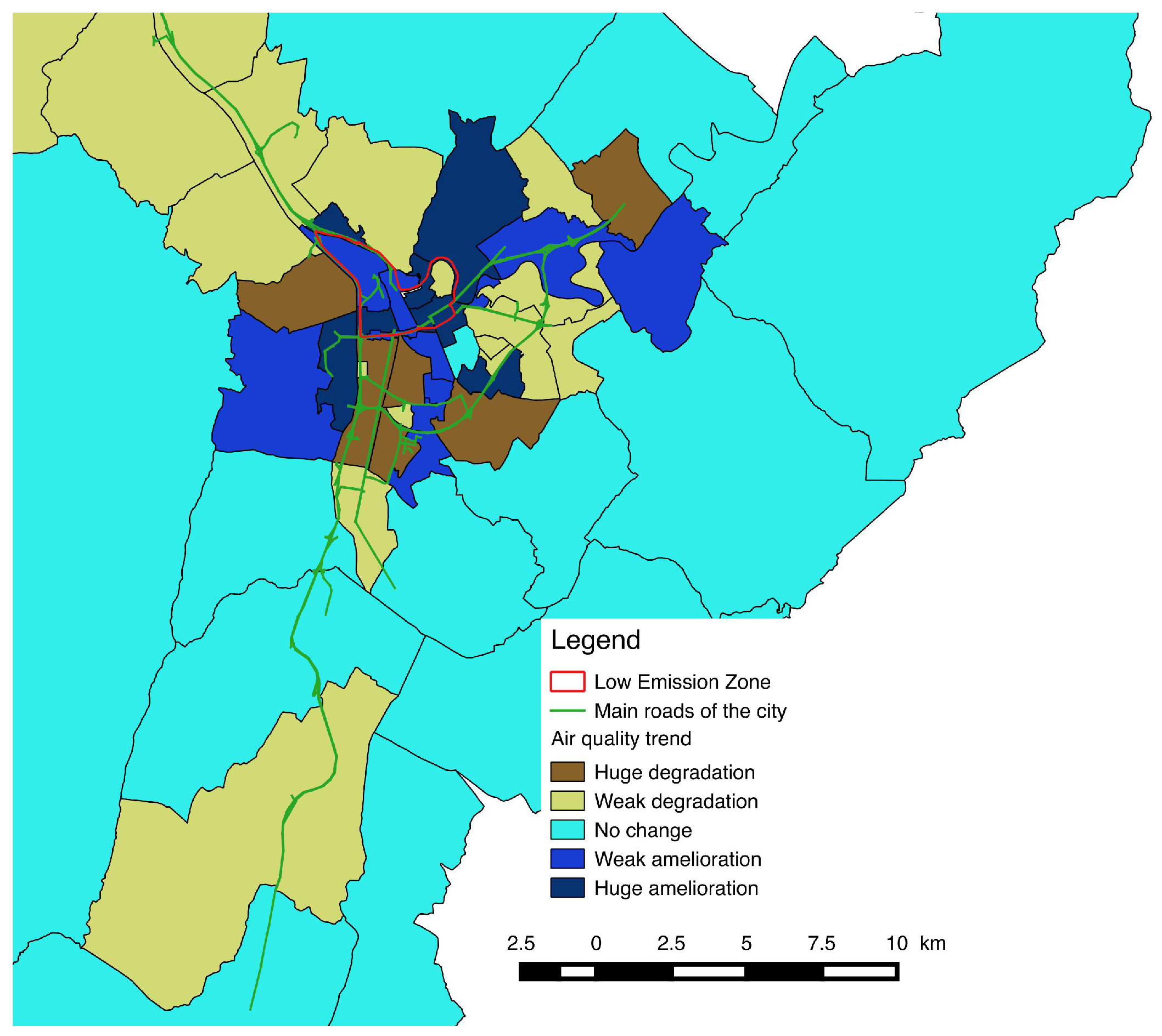
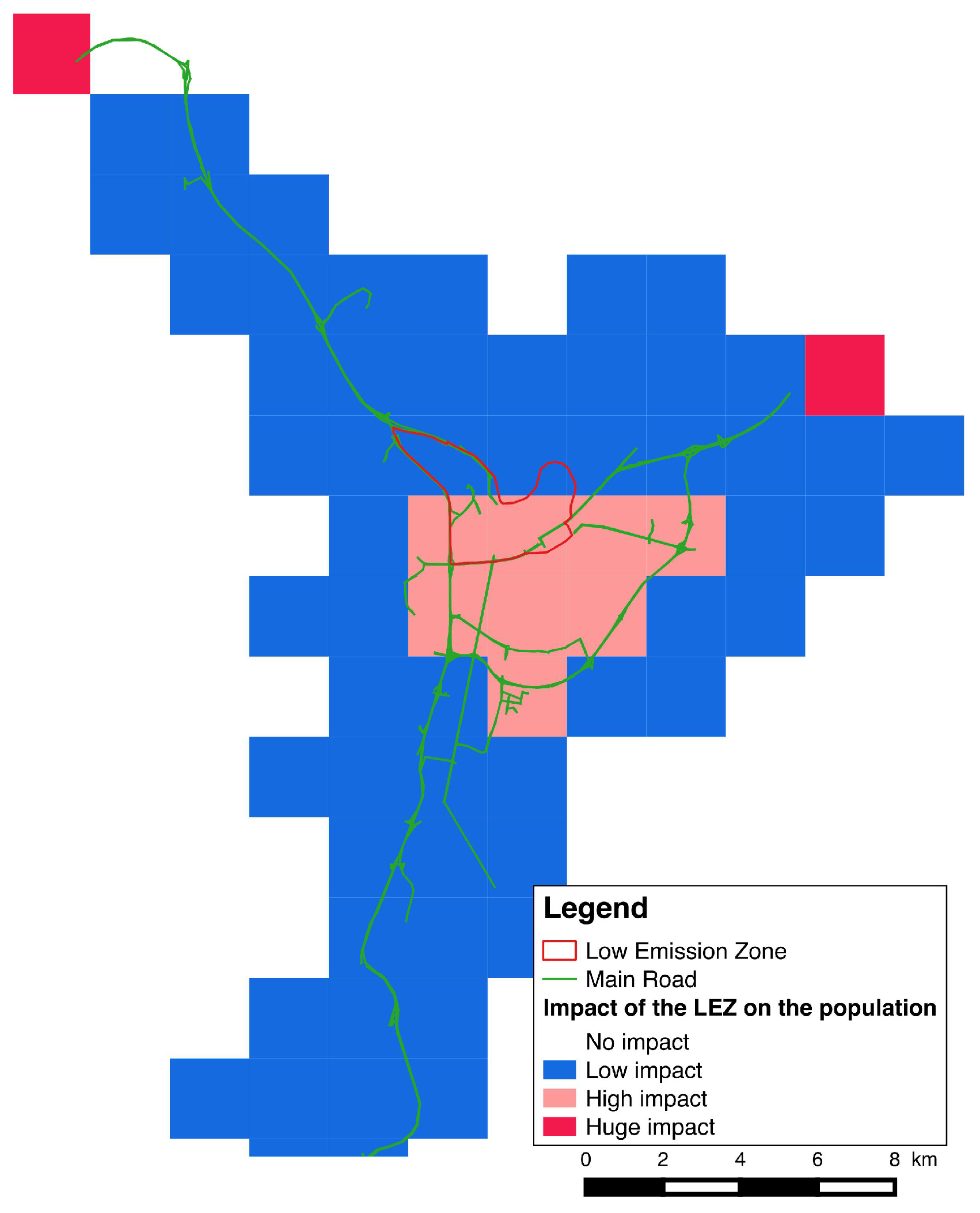
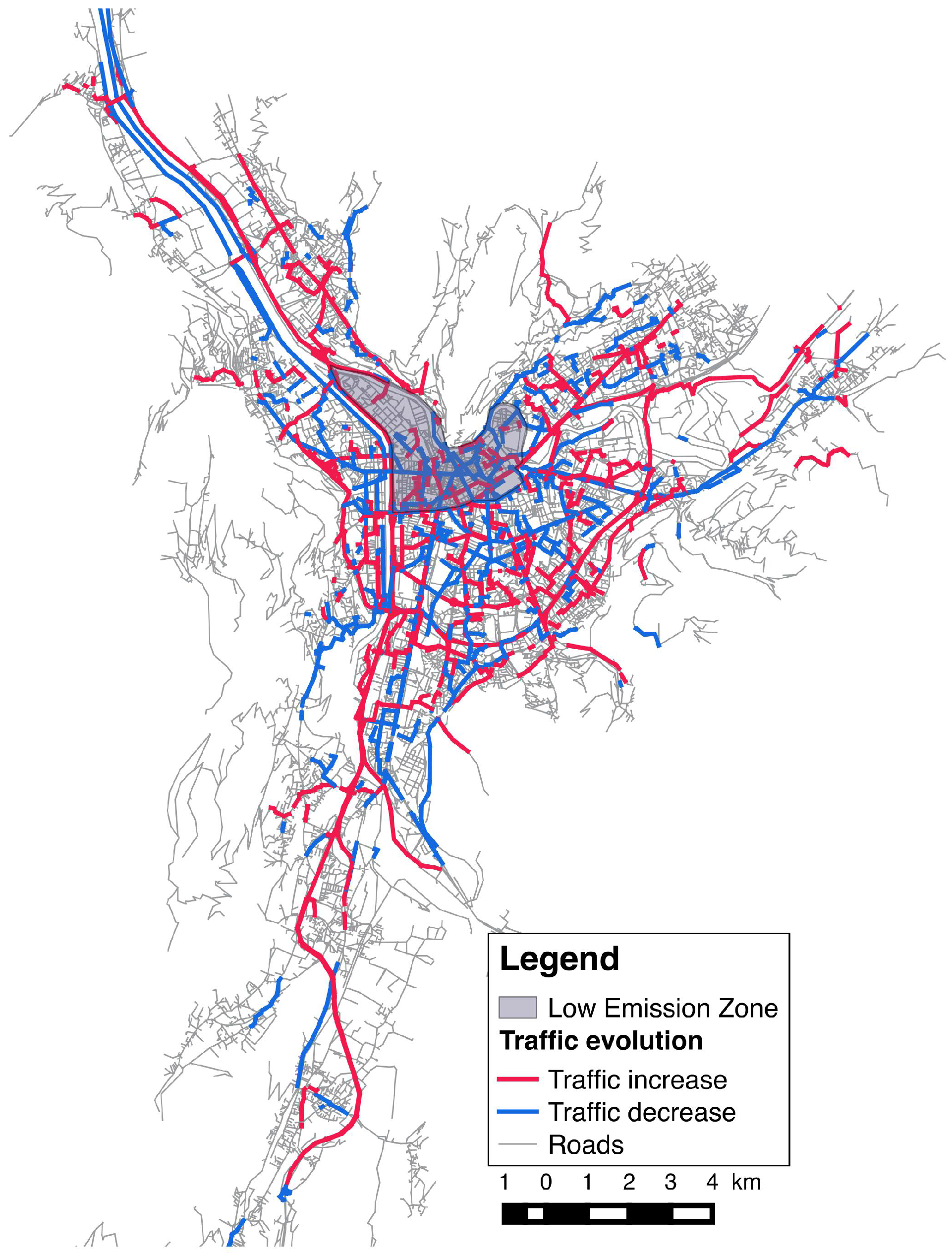
5. Simulation and Results
- in which extent the LEZ area impact the traffic and the air quality in the different zones of the city;
- how the population will be impacted considering their capacity to maintain their daily programs and mobility.


6. Conclusions
Acknowledgments
Author Contributions
Conflicts of Interest
References
- Chapin, F.S. Human Activity Patterns in the City: Things People Do in Time and in Space; John Wiley & Sons: New York, NY, USA, 1974; p. 272. [Google Scholar]
- Hägerstrand, T. What about people in regional science? Pap. Reg. Sci. Assoc. 1970, 24, 7–21. [Google Scholar] [CrossRef]
- Nally Mc, M.G.; Rindt, C. The Activity-Based Approach. In Handbook of Transport Modelling, 2nd ed.; Elsevier: London, UK, 2008. [Google Scholar]
- Greaves, S.; Stopher, P. A Synthesis of GIS and Activity-Based Travel-Forecasting. Geogr. Syst. 1998, 5, 59–90. [Google Scholar]
- Lenntorp, B. Paths in space-time environments: A time geographic study of movement possibilities of indviduals. Environ. Plan. A 1977, 9, 961–972. [Google Scholar]
- Jones, P.M. New Approaches to Understanding Travel Behaviour: The Human Activity Approach; Redwood Burn Ltd.: London, UK, 1979; pp. 55–80. [Google Scholar]
- Recker, M.G. A Model of Complex Travel Behavior: Part I—Theoretical Development. Transp. Res. A Gen. 1986, 20, 307–318. [Google Scholar] [CrossRef]
- Gärling, T.; Kwan, M.-P.; Golledge, R. Computational process modeling of household activity scheduling. Trans. Res. B 1994, 28, 355–364. [Google Scholar] [CrossRef]
- Axhausen, K.W.; Goodwin, P.B. EUROTOPP, towards a Dynamic and Activity-Based Modelling Framework. Adv. Telemat. Road Transp. 1991, 2, 1020–1039. [Google Scholar]
- Stopher, P.R.; Hartgen, D.T.; Li, Y. SMART: Simulation Model for Activities, Resources and Travel. Transportation 1996, 23, 293–312. [Google Scholar] [CrossRef]
- Kitamura, R.; Fujii, S. Two Computational Process Models of Activity-Travel Behavior. In Theoretical Foundations of Travel Choice Modeling; Emerald Group Publishing Limited: Oxford, UK, 1998; pp. 251–279. [Google Scholar]
- Arentze, T.; Timmermans, H. Albatross: A Learning Based Transportation Oriented Simulation System; Eindhoven: Eirass, The Netherlands, 2000. [Google Scholar]
- Benenson, I.; Torrens, P. Geographic Automata Systems. Int. J. Geogr. Inf. Sci. 2005, 19, 385–412. [Google Scholar]
- Barrett, C.; Bisset, K.; Jacob, R.; Konjevod, G.; Marathe, M. Classical and Contemporary Shortest Path Problems in Road Networks: Implementation and Experimental Analysis of the TRANSIMS Router. In Proceedings of the Algorithms-ESA, Rome, Italy, 17–21 September 2002; pp. 313–319.
- Balmer, M.; Nagel, K.; Raney, B. Large-Scale Multi-Agent Simulations for Transportation Applications. J. Intell. Transp. Syst. 2004, 8, 205–221. [Google Scholar] [CrossRef]
- Huynh, N.; Perez, P.; Berryman, M.; Barthelemy, J. Simulating Transport and Land Use Interdependencies for Strategic Urban Planning—An Agent Based Modelling Approach. Systems 2015, 3, 177–210. [Google Scholar] [CrossRef]
- Ferber, J. Multi-Agent System: An Introduction to Distributed Artificial Intelligence; Addison Wesley Longman: Harlow, UK, 1999. [Google Scholar]
- Chu, Y.; Wassick, J.M.; You, F. Efficient scheduling method of complex batch processes with general network structure via agent-based modeling. AIChe J. 2013, 59, 2884–2906. [Google Scholar] [CrossRef]
- Irit GenStar. Available online: http://www.irit.fr/genstar/ (accessed on 14 January 2016).
- Tversky, A. Elimination by aspects: A theory of choice. Psychol. Rev. 1972, 79, 281–299. [Google Scholar] [CrossRef]
- Train, K. Discrete Choice Methods with Simulation, 2nd ed.; Cambridge University Press: Cambridge, UK, 2009. [Google Scholar]
- Ben-Akiva, M.; Bierlaire, M. Discrete choice methods and their applications to short term travel decisions. In Handbook of Transportation Science; Hall, R., Ed.; Kluwer: Boston, MA, USA, 1999; pp. 5–34. [Google Scholar]
- Ben-Akiva, M.; Lerman, S.R. Discrete Choice Analysis: Theory and Application to Travel Demand; MIT Press: Cambridge, MA, USA, 1985. [Google Scholar]
- Gama Platform on Github. Available online: https://github.com/gama-platform/gama/wiki (accessed on 14 January 2016).
- Grignard, A.; Taillandier, P.; Gaudou, B.; Vo, D.-A.; Huynh, N.-Q.; Drogoul, A. GAMA 1.6: Advancing the Art of Complex Agent-Based Modeling and Simulation. In PRIMA’2013: Principles and Practice of Multi-Agent Systems, Lecture Notes in Computer Science; Springer: Berlin Heidelberg, Germany, 2013; Volume 8291, pp. 117–131. [Google Scholar]
- Nagel, K.; Schrekenberg, M. A cellular automaton model for freeway traffic. J. Phys. I 1992, 2, 2221–2229. [Google Scholar] [CrossRef]
- Lighthill, M.J.; Whitham, G.B. On kinematic waves II: A theory of traffic flow on long, crowded roads. Proc. R. Soc. Lond. Ser. A 1955, 229, 317–345. [Google Scholar] [CrossRef]
- Richards, P.I. Shock waves on the highway. Oper. Res. 1956, 4, 42–51. [Google Scholar] [CrossRef]
- Underwood, R. Speed, Volume, and Density Relationship Quality and Theory of Trac Flow; Yale Bureau of Highway Traffic: New Haven, CT, USA, 1961. [Google Scholar]
- UK Ministry of Transport. Available online: https://www.gov.uk/government/uploads/system/uploads/attachment_data/file/4258/viewer.xls (accessed on 15 January 2016).
- WHO air quality guidelines. Available online: http://www.who.int/mediacentre/news/releases/2014/air-quality/en/ (accessed on 15 January 2016).
- Charleux, L. Contingencies of environmental justice: The case of individual mobility and Grenoble’s low-emission zone. In Urban Geography; Taylor & Francis: London, UK, 2014; pp. 1938–2847. [Google Scholar]
© 2016 by the authors; licensee MDPI, Basel, Switzerland. This article is an open access article distributed under the terms and conditions of the Creative Commons by Attribution (CC-BY) license (http://creativecommons.org/licenses/by/4.0/).
Share and Cite
Fosset, P.; Banos, A.; Beck, E.; Chardonnel, S.; Lang, C.; Marilleau, N.; Piombini, A.; Leysens, T.; Conesa, A.; Andre-Poyaud, I.; et al. Exploring Intra-Urban Accessibility and Impacts of Pollution Policies with an Agent-Based Simulation Platform: GaMiroD. Systems 2016, 4, 5. https://doi.org/10.3390/systems4010005
Fosset P, Banos A, Beck E, Chardonnel S, Lang C, Marilleau N, Piombini A, Leysens T, Conesa A, Andre-Poyaud I, et al. Exploring Intra-Urban Accessibility and Impacts of Pollution Policies with an Agent-Based Simulation Platform: GaMiroD. Systems. 2016; 4(1):5. https://doi.org/10.3390/systems4010005
Chicago/Turabian StyleFosset, Pierre, Arnaud Banos, Elise Beck, Sonia Chardonnel, Christophe Lang, Nicolas Marilleau, Arnaud Piombini, Thomas Leysens, Alexis Conesa, Isabelle Andre-Poyaud, and et al. 2016. "Exploring Intra-Urban Accessibility and Impacts of Pollution Policies with an Agent-Based Simulation Platform: GaMiroD" Systems 4, no. 1: 5. https://doi.org/10.3390/systems4010005
APA StyleFosset, P., Banos, A., Beck, E., Chardonnel, S., Lang, C., Marilleau, N., Piombini, A., Leysens, T., Conesa, A., Andre-Poyaud, I., & Thevenin, T. (2016). Exploring Intra-Urban Accessibility and Impacts of Pollution Policies with an Agent-Based Simulation Platform: GaMiroD. Systems, 4(1), 5. https://doi.org/10.3390/systems4010005