
A Modular Modelling Framework for Hypotheses Testing in the Simulation of Urbanisation

 ,
,
Abstract
:1. Introduction
2. A Catalogue of Possible Mechanisms of Urbanisation
“It may also be useful to think of complex geographical models as extensions of thought experiments, where the necessary and contingent implications of theories can be examined. Further, admitting that “all models are wrong” is akin to the realisation in post-structural social science that multiple competing accounts of the same settings are possible, and that faced with a diversity of accounts the context and intent of each must be an important element in the evaluation process”([7] p. 291).
2.1. Competing Theories
- Spatial Interactions and diffusion allow for the exchange of informations, monies, goods and people. It thus makes cities co-evolve in time and adapt collectively to changing economic and innovation cycles through competition and cooperation, resulting in some complementarity of their specialisation. These local interactions and their consequences on the regular organisation of the system as a whole under spatial constraints could be thought of as “complex systems effects”.
- Size effects like agglomeration economies and urbanisation externalities illustrate a very direct and self-reinforcing cause for hierarchical differentiation.
- Site effects explain the spatial location of growth processes around resource-rich areas for the related innovation cycle.
- Situation effects illustrate the importance of the neighbouring relational environment (potential field, network accessibility, etc.) on a city’s pattern of growth.
- Territorial effects account for some exogenous (policy) shocks and the solidarity of urban trajectories in a common political space (through redistributive processes for example).
2.2. Empirical Results from the Literature
- Spatial Interactions are tricky to measure because of the variety and non-commensurability of flows circulating between cities at various temporalities. Until recently, the diffusion of innovations (agricultural techniques [40], telephone lines [41] or newspapers [42]) served as a proxy for these interactions. Since the development of various volumes of high velocity data, actual interactions (like phone calls [43]) have confirmed for example the relevance of the gravity model to describe inter-city interactions.
- Size effects on urban growth and differentiation were revealed by a persistent empirical correlation between growth rates and city sizes over long periods of time. All over the 19th century, Robson ([41] p. 79) measured a positive coefficient between the log of English and Welsh cities’ population and their gross ten-year growth rates (from a minimum of +1.47 between 1861 and 1871 to a maximum of +8.53 points in percentage between 1821 and 1831). This correlation is found for French cities as well [44]. The size effect finally relates to the stability of the rank position of large cities (by comparison with the fluctuations of smaller cities).
- Site effects were classically approached by estimating the surplus of growth associated with a localised resource (typically, deposits of natural materials, such as coal or gas). In the Soviet urban system of the 1920s–1930s, the location of a city on a coal deposit was associated with a surplus of 1.15 points in percentage of average demographic growth per annum, everything else being equal. A surplus over 0.5 point is observed nowadays (1989–2010) for oil and gas deposits [45]. In the USA, Black and Henderson [46] estimate that the coastal location (e.g., a resource for tourism) is associated with a significantly higher ten-year growth rates of three to five points.
- Situation effects can be revealed by the spatial autocorrelation of growth or the co-evolution between transportation networks and urban networks. In the first case, Hernando et al. [47] found a characteristic distance for spatial autocorrelation of growth rates of 215 km for American counties and of 80 km for Spanish cities. As for transportation dynamics, Bretagnolle [48] measured the correlation between accessibility and growth rates for French cities in the last two centuries. She finds that cities that were weakly connected (by any transportation network: road, rail or air) in 1900 and stayed isolated in 2002 grew slower (0.94% on average per annum between 1900 and 2002) than cities that became motorway nodes (1.21%) or multimodal hubs (1.69%). Likewise, well connected cities at the beginning of the period tended to grow faster than the first category.
- Territorial effects can be approached empirically by relating political statuses to dynamics of growth. In developing countries, regional capitals were found to grow significantly faster by 0.5 to 1 point of annual average growth rate in the 1960s [49] and the 1990s [50]. In the Former Soviet Union, the regional status of capital has proven important to predict urban growth [51], the coefficient regressed against growth rates over time ranges from +0.24 point between 1989 and 2002 to +1.88 between 1926 and 1939 [45]. Besides, cities that belong to the same territory have shown an increased pattern of synchronicity in their growth and decline trajectories from the 1980s on, suggesting evidence of both political shocks and territorial solidarity in the spatial distribution of urban growth.
2.3. A Case Study : The Former Soviet Union
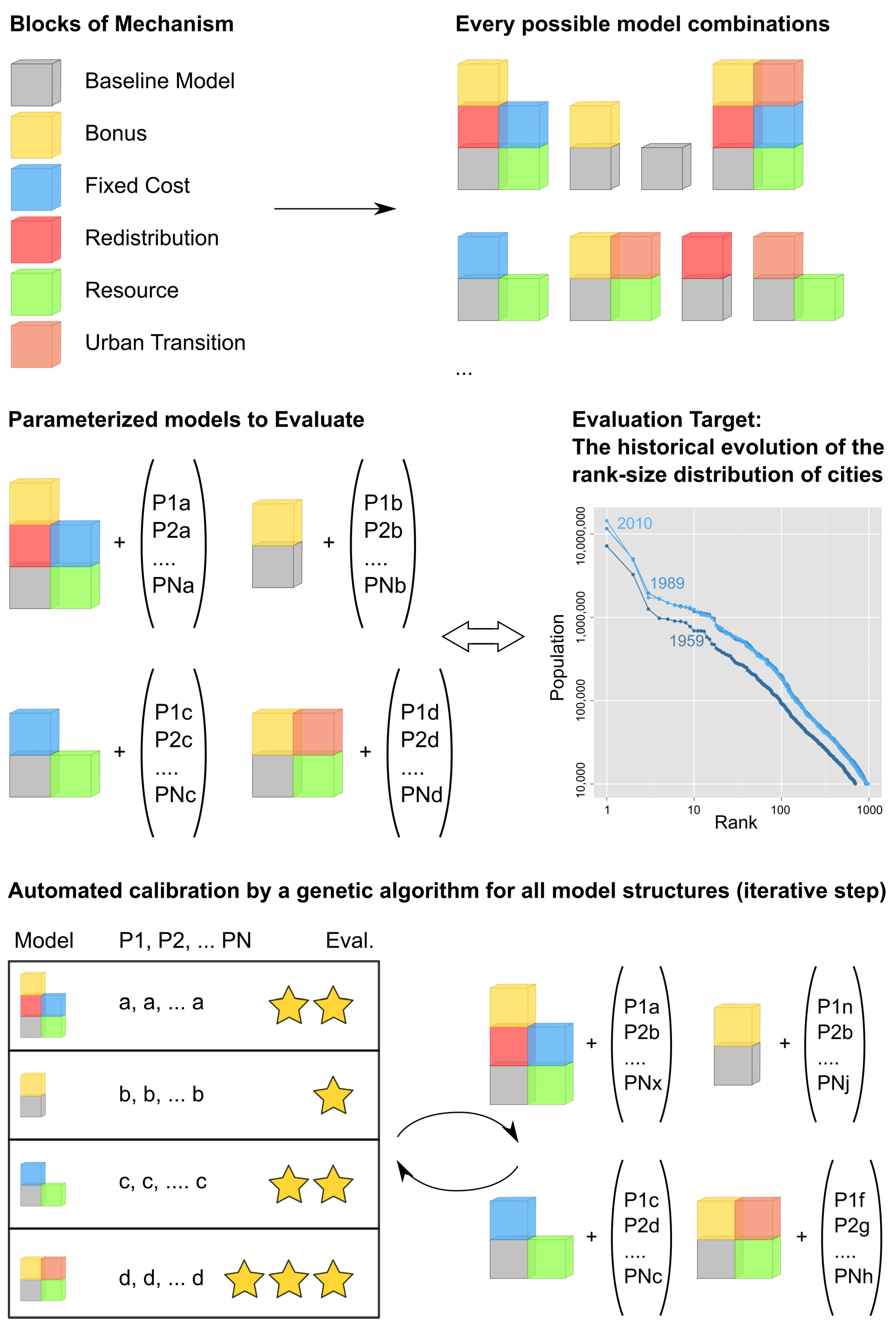
3. Modular Multimodelling Experiment
3.1. Overview
- Each city updates its economic variables based on its current population;
- Cities interact (i.e., exchange product) with other cities according to they supply, demand and distance;
- Each city updates its wealth based on the results of its interactions;
- A simulation step ends when each city updates its population.
3.2. Design Concepts
3.3. Implementing Mechanisms as Building Blocks (Details)
3.3.1. The Baseline Model
- Each city interacts with other cities according to the intensity of their potential Equation (9). For two distinct cities i and j, the computation of the interaction potential consists in confronting the supply of i Equation (11) to the demand of j with an equation borrowed to the gravity model Equation (12).
3.3.2. Mechanism Increments
- The mechanism that accounts for interactions benefits at the intercity level is the one called bonus. It
“[...] features a non-zero sum game [...], rewarding cities who effectively interact with others rather than internally. We assume that the exchange of any unit of value is more profitable when it is done with another city, because of the potential spillovers of technology and information [54].”
- A mechanism related to situation advantages is called fixed costs. It ensures that the situation of each city in the system is taken into account in its interactions with other cities.
“Every interurban exchange generates a fixed cost (the value of which is described by the free parameter ). This implies two features that make the model more realistic: first, no exchange will take place between two cities if the potential transacted value is under a certain threshold ; second, cities will select only profitable partners and not exchange with every other cities. This mechanism plays the role of a condition before the exchange” [54].
- Site effects are targeted by the resource mechanism: site advantages are particularised in this model by natural resource deposits (more specifically: coal deposits C on the one hand, and oil and gas deposits O on the other hand). The assumption is made that if the city i is located on some coal or oil deposits ( or ), the city benefits from the advantage granted by the extraction activity. The capacity of extraction depends on the capital (wealth) of the city and takes the form of a wealth multiplier for each resource Equation (22) after Equation (14):
- Territorial and political effects are formalised by the redistribution mechanism. It allows for a redistribution of wealth between cities of the same territory R (region or State). To do so, territorial taxes are collected in each city , as a proportion of their wealth. The total amount of taxes collected is Equation (23):
- Finally, territorial and situation explanations are mixed in the urban transition mechanism. To account for the different opportunities of cities to attract rural migrants in the different regions, we model the evolution of the urban transition curves over time. As shown empirically [45], 100 out of the 108 regions of the Former Soviet Union have followed the scheme of the urban transition. It means that their urbanisation rate (in %) has followed a logistic function over time t Equation (27):
3.4. Technical Modular Implementation
               Listing 1: Object oriented specialisation.
		abstract class C extends A with B {
		 def a(x : Double) : Double
		 def b(x : Double) : Double
		 def c(x : Double) = /* Compute something using a and b * /
		}
		class C1 extends C {
		 def a(x : Double) = /* Some implementation of a  */
		 def b(x : Double) = /* Some implementation of b  */
		}
		       Listing 2: Mixin in Scala.
		trait A {
		 def a(x : Double) : Double
		}
		trait B {
		 def b(x : Double) : Double
		}
		trait C extends A with B {
		 def c(x : Double) = /* Compute something using a and b */
		}
		// Implementation 1 of trait A
		trait A1 extends A {
		def a(x : Double) = /* Some implementation */
		}
		// Implementation 2 of trait A
		trait A2 extends A {
		 // Parameter p0 used in this version of a
		 def p0 : Double
		 def a(x : Double) = /* Some implementation using p0 */
		}
		// Implementation 2 of trait B
		trait B2 extends B {
		 def b(x : Double) = /* Some implementation */
		}
		val instance 1 =
		 new C with A1 with B2 {}
		val instance 2 =
		 new C with A2 with B2 {
		  // Value for parameter p0 of trait A2
		  def p0 = 1.0
		 }
		       Listing 3: Example of generated code.
		def model (index : Int , parameters : Seq[Double]) =
		 index match {
		  case 0 =>
		   new Model with T11 with T21 with . . . {
		    def p0 = parameters(0)
		    def p1 = parameters(1)
		    ...
		   }
		  case 1 =>
		   new Model with T11 with T22 with ... {
		    def p0 = parameters(0)
		    def p1 = parameters(1)
		    ...
		   }
		  case 2 => ...
		 }

3.5. Calibrating a Multi-Model
“Whatever changes occur in the institutional, political and social context of computational models, the question of how to learn from models remains. It is clear that assessment of the accuracy of a model as a representation must rest on argument about how competing theories are represented in its workings, with calibration and fitting procedures acting as a check on reasoning”([7] p. 291).
4. Results: Hypothesis Testing to Explain Urbanisation in the Former Soviet Union
- 1
- Which is the most parsimonious model to simulate the evolution of cities before and after the collapse of the Soviet Union? A way to answer this question is to restrict the set of results to the five model structures that correspond to the a mix of two mechanisms: the baseline model + one additional mechanism (for example: resource extraction). That leaves us with parameter sets and 250 performance values δ for each time period analysed. We look at the lowest distance to empirical data achieved in this set of results, and identify the corresponding model structure (the additional mechanism involved) and parameter values as the best performing ones.

| Parameter Name | Value | Mechanism |
|---|---|---|
| economicMultiplier | 0.002193758 | Baseline |
| populationToWealth | 1.000184755 | Baseline |
| sizeEffectOnSupply | 1.053943022 | Baseline |
| sizeEffectOnDemand | 1.000000000 | Baseline |
| wealthToPopulation | 0.203567639 | Baseline |
| distanceDecay | 1.872702086 | Baseline |
| ruralMultiplier | 0.034975771 | UrbanTransition |
| Normalized δ | n cities | Time steps |
| 0.01423387 | 1145 | 30 |
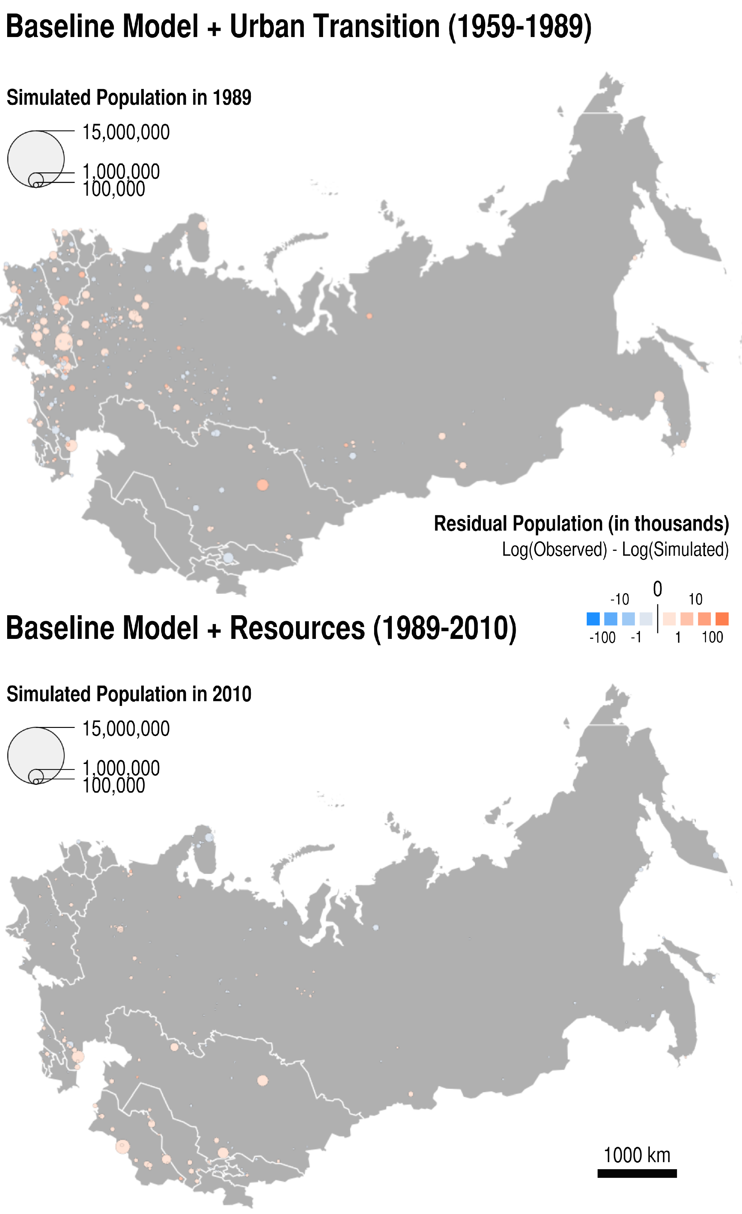
| Parameter Name | Value | Mechanism |
|---|---|---|
| economicMultiplier | 0.502616330 | Baseline |
| populationToWealth | 1.124963276 | Baseline |
| sizeEffectOnSupply | 1.002982515 | Baseline |
| sizeEffectOnDemand | 1.000808442 | Baseline |
| wealthToPopulation | 0.699943763 | Baseline |
| distanceDecay | 1.475836151 | Baseline |
| oilAndGazEffect | 0.017066495 | Resources |
| coalEffect | −0.011792670 | Resources |
| Normalized δ | n cities | Time steps |
| 0.005180008 | 1822 | 21 |
- 2
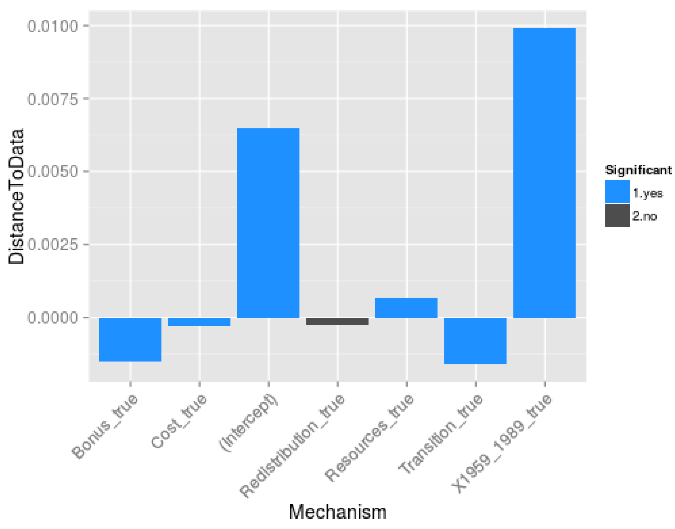
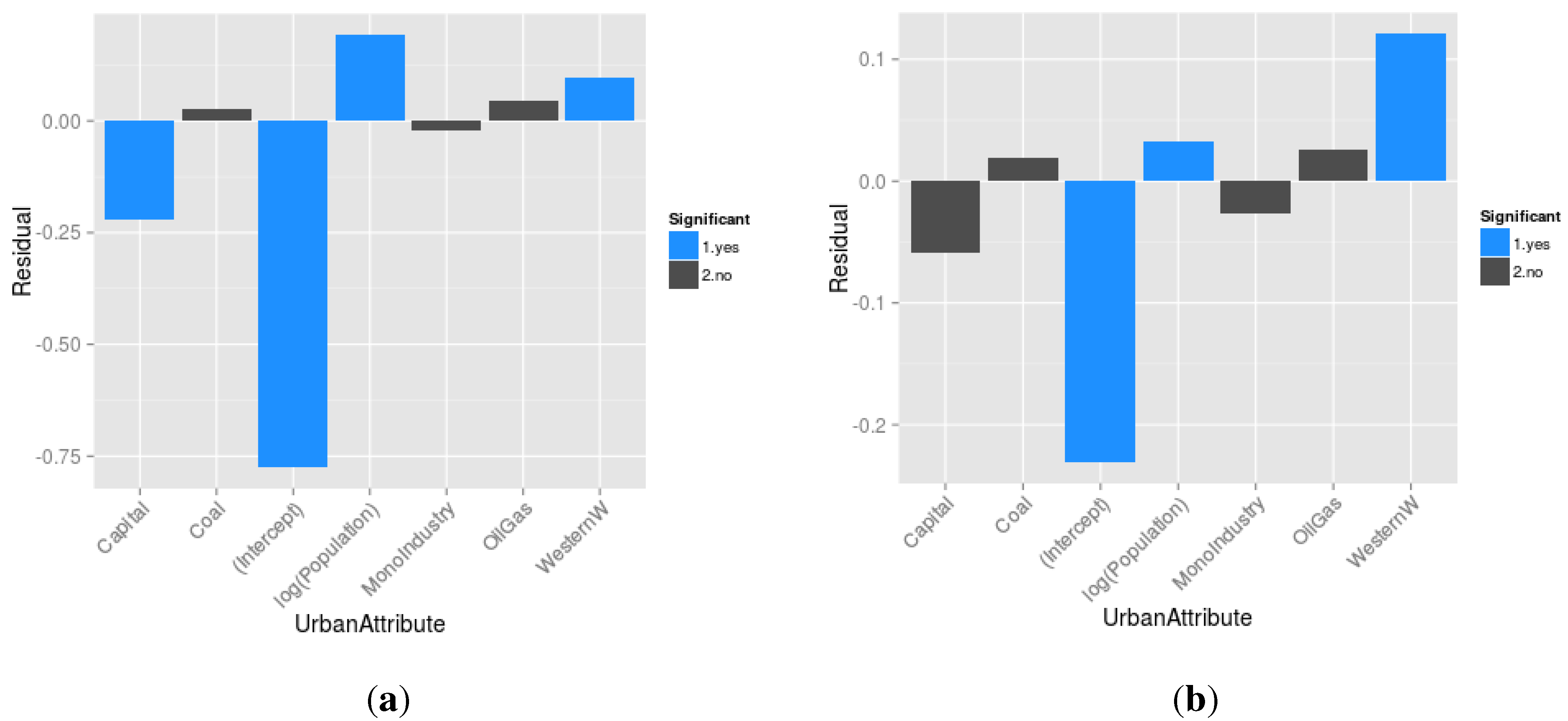
- Which are the mechanisms (and mechanisms’ interactions) that are essential to model the Soviet and post-Soviet urbanisation patterns? To address this question, we statistically analyse the results of the multicalibration (3200 sets of parameters, the best 50 of each model structure for each time period) to evaluate the contribution of each mechanism (everything else being equal in the model structure) to the reduction of distance between simulated and observed demographic data for each city. More specifically, we regress the distance to data δ against the mechanism composition of the model, following Equation (30):

- 3
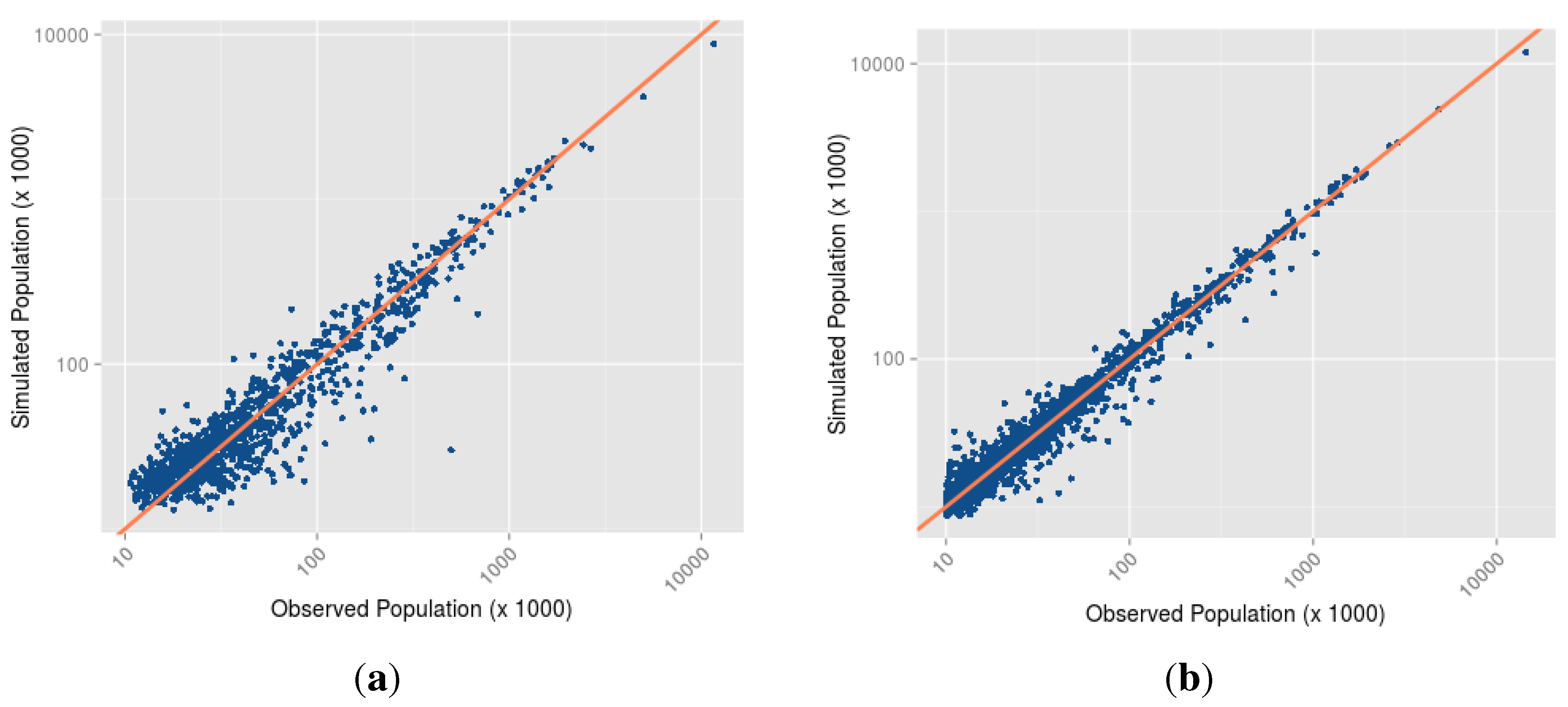
- What are the cities that resist modelling? In other words, what are the cities that are too specific to be modelled by any of the mechanisms implemented? To answer this last question, we statistically analyse the difference between the log of the population observed and the log of the population simulated at the last evaluation Census date for cities included in the simulation, with respect to their locational and functional attributes. The models for which we present the results below contains all the implemented mechanisms, and are applied to the two periods of enquiry.
| Positive Residuals | ||
|---|---|---|
| City | Observed Pop. | Simulated Pop. |
| Naberezhnye Tchelny | 500,000 | 30,000 |
| Volgodonsk | 191,000 | 36,000 |
| Chajkovskij | 86,000 | 19,000 |
| Toljatti | 685,000 | 158,000 |
| Bratsk | 285,000 | 73,000 |
| Balakovo | 197,000 | 52,000 |
| Tihvin | 71,000 | 20,000 |
| Chervonograd | 72,000 | 21,000 |
| Obninsk | 111,000 | 32,000 |
| Staryjoskol | 174,000 | 53,000 |
| Negative Residuals | ||
| City | Observed Pop. | Simulated Pop. |
| Zaozernyj | 16,000 | 54,000 |
| Gremjachnsk | 21,000 | 56,000 |
| Atakent/Ilitch | 15,000 | 38,000 |
| Kizel | 37,000 | 88,000 |
| Cheremhovo | 74,000 | 172,000 |
| Ilanskij | 18,000 | 42,000 |
| Gornoaltajsk | 46,000 | 102,000 |
| Volchansk | 15,000 | 32,000 |
| Zujevka | 16,000 | 35,000 |
| Taldykorgai | 138,000 | 296,000 |
| Positive Residuals | ||
|---|---|---|
| City | Observed Pop. | Simulated Pop. |
| Mirnyja | 41,000 | 12,000 |
| Sertolovo | 48,000 | 16,000 |
| Beineu | 32,000 | 11,000 |
| Govurdak | 76,000 | 28,000 |
| Serdar/Gyzylarbat | 98,000 | 37,000 |
| Bayramaly | 131,000 | 53,000 |
| Sarov | 92,000 | 39,000 |
| Turkmenabat/Tchardjou | 427,000 | 185,000 |
| Astana/Tselinograd | 613,000 | 278,000 |
| Dashougouz | 275,000 | 126,000 |
| Sovetabad | 11,000 | 33,000 |
| Zhanatas | 21,000 | 50,000 |
| Krasnozavodsk | 13,000 | 31,000 |
| Gagra | 11,000 | 25,000 |
| Nevelsk | 12,000 | 26,000 |
| Arkalyk | 28,000 | 59,000 |
| Chyatura | 14,000 | 28,000 |
| Aleksandrovsk Sahalinsk | 11,000 | 21,000 |
| Uglegorsk | 10,000 | 20,000 |
| Baikonyr | 36,000 | 67,000 |
5. Discussion
“Despite the fact that the experience of individual cities has become more varied internationally (at least within what might be called the mature economies) there is stronger evidence of a predictable pattern of change, determined by common causal factors, than might be expected given the diversity and variety of cities”([15] p. 1342).
6. Conclusions
Acknowledgments
Author Contributions
Conflicts of Interest
References
- Batty, M. Fifty years of urban modeling: Macro-statics to micro-dynamics. In The Dynamics of Complex Urban Systems; Springer: Heidelberg, German, 2008; pp. 1–20. [Google Scholar]
- Heppenstall, A.J.; Crooks, A.T.; See, L.M.; Batty, M. Agent-Based Models of Geographical Systems; Springer Science & Business Media: London, UK, 2012. [Google Scholar]
- Pumain, D.; Sanders, L. Theoretical principles in inter-urban simulation models: A comparison. Environ. Plann. A 2013, 45, 2243–2260. [Google Scholar] [CrossRef]
- Carley, K.M. (1999). On Generating Hypotheses Using Computer Simulations. DTIC Document. Available online: http://www.dtic.mil/cgi-bin/GetTRDoc?AD=ADA458065 (accessed on 25 November 2015).
- Hedström, P.; Ylikoski, P. Causal mechanisms in the social sciences. Annu. Rev. Sociol. 2010, 36, 49–67. [Google Scholar] [CrossRef]
- Von Bertalanffy, L. General System Theory: Foundations, Development, Applications; Braziller: New York, NY, USA, 1968. [Google Scholar]
- O’Sullivan, D. Complexity science and human geography. Trans. Inst. Br. Geogr. 2004, 29, 282–295. [Google Scholar] [CrossRef]
- Rossiter, S.; Noble, J.; Bell, K.R.W. Social simulations: Improving interdisciplinary understanding of scientific positioning and validity. J. Artif. Soc. Soc. Simul. 2010, 13, 1–10. [Google Scholar] [CrossRef]
- Elsenbroich, C. Explanation in agent-based modelling: Functions, causality or mechanisms? J. Artif. Soc. Soc. Simul. 2012, 15, 1–9. [Google Scholar] [CrossRef]
- Grüne-Yanoff, T. The explanatory potential of artificial societies. Synthese 2009, 169, 539–555. [Google Scholar] [CrossRef]
- Chérel, G.; Cottineau, C.; Reuillon, R. Beyond Corroboration: Strengthening Model Validation by Looking for Unexpected Patterns. PLoS ONE 2015, 10, e0138212. [Google Scholar] [CrossRef] [PubMed]
- Kaldor, N. Capital accumulation and economic growth. In The Theory of Capital; Macmillan: London, UK, 1961. [Google Scholar]
- Pumain, D. Pour une théorie évolutive des villes. Espace Géogr. 1997, 26, 119–134, in French. [Google Scholar] [CrossRef]
- Krugman, P. Confronting the mystery of urban hierarchy. J. Jpn. Int. Econ. 1996, 10, 399–418. [Google Scholar] [CrossRef]
- Cheshire, P. Trends in sizes and structures of urban areas. Handb. Reg. Urban Econ. 1999, 3, 1339–1373. [Google Scholar]
- Pumain, D. Hierarchy in the Natural and Social Sciences; Methodos Series; Springer: Heidelberg, German, 2006. [Google Scholar]
- Auerbach, F. Das gesetz der bevolkerungskonzentration. Petermanns Geogr. Mitt. 1913, 59, 73–76. [Google Scholar]
- Lotka, A.J. Elements of Physical Biology; William & Wilkins: Baltimore, MD, USA, 1925. [Google Scholar]
- Singer, H.W. The “courbe des populations.” A parallel to Pareto’s Law. Econ. J. 1936, 46, 254–263. [Google Scholar] [CrossRef]
- Zipf, G.K. Human Behavior and the Principle of Least Effort; Addison-Wesley: Cambridge, MA, USA, 1949. [Google Scholar]
- Berry, B.J. City size distributions and economic development. Econ. Dev. Cult. Chang. 1961, 9, 573–588. [Google Scholar] [CrossRef]
- Eeckhout, J. Gibrat’s law for (all) cities. Am. Econ. Rev. 2004, 5, 1429–1451. [Google Scholar] [CrossRef]
- Gibrat, R. Les Inégalités Économiques; Sirey: Paris, France, 1931; in French. [Google Scholar]
- Clauset, A.; Shalizi, C.R.; Newman, M.E. Power-law distributions in empirical data. SIAM Rev. 2009, 51, 661–703. [Google Scholar] [CrossRef]
- Mitzenmacher, M. A brief history of generative models for power law and lognormal distributions. Internet Math. 2004, 1, 226–251. [Google Scholar] [CrossRef]
- Simon, H.A. On a class of skew distribution functions. Biometrika 1955, 42, 425–440. [Google Scholar] [CrossRef]
- Krugman, P. The Self-Organizing Economy; Blackwell: Oxford, UK, 1996. [Google Scholar]
- Pumain, D. (2004). Scaling laws and urban systems. Santa Fe Institute, WP, (04-02). Available online: http://samoa.santafe.edu/media/workingpapers/04-02-002.pdf (accessed on 25 November 2015).
- Gabaix, X. Zipf’s law for cities: An explanation. Q. J. Econ. 1999, 114, 739–767. [Google Scholar] [CrossRef]
- Dimou, M.; Schaffar, A. Les théories de la croissance urbaine. Rev. D’écon. Politique 2011, 121, 179–207, in French. [Google Scholar] [CrossRef]
- Henderson, J.V. The sizes and types of cities. Am. Econ. Rev. 1974, 64, 640–656. [Google Scholar]
- Krugman, P. Urban concentration: The role of increasing returns and transport costs. Int. Reg. Sci. Rev. 1996, 19, 5–30. [Google Scholar] [CrossRef]
- Allen, P.M.; Sanglier, M. Urban evolution, self-organization, and decisionmaking. Environ. Plan. A 1981, 13, 167–83. [Google Scholar] [CrossRef]
- Bura, S.; Guérin-Pace, F.; Mathian, H.; Pumain, D.; Sanders, L. Multiagent systems and the dynamics of a settlement system. Geogr. Anal. 1996, 28, 161–178. [Google Scholar] [CrossRef]
- Weidlich, W.; Haag, G. Concepts and Models of a Quantitative Sociology. The Dynamics of Interacting Populations; Springer: Berlin, Germany, 1983. [Google Scholar]
- Christaller, W. Die zentralen Orte in Süddeutschland: Eine ökonomisch-geographische Untersuchung über die Gesetzmässigkeit der Verbreitung und Entwicklung der Siedlungen mit städtischen Funktionen; Verlag Gustav Fischer: Jena, German, 1933. [Google Scholar]
- Ullman, E. A theory of location for cities. Am. J. Sociol. 1941, 6, 853–864. [Google Scholar] [CrossRef]
- Duranton, G.; Puga, D. Nursery cities: Urban diversity, process innovation, and the life cycle of products. Am. Econ. Rev. 2001, 91, 1454–1477. [Google Scholar] [CrossRef]
- Pumain, D.; Paulus, F.; Vacchiani-Marcuzzo, C.; Lobo, J. An evolutionary theory for interpreting urban scaling laws. Cybergeo Eur. J. Geogr. 2006, 343, 1–22. [Google Scholar] [CrossRef]
- Hägerstrand, T. Innovation Diffusion as a Spatial Process; University of Chicago Press: Chicago, IL, USA, 1968. [Google Scholar]
- Robson, B.T. Urban Growth: An Approach; Routledge: London, UK, 1973. [Google Scholar]
- Pred, A.R. The Growth and Development of Systems of Cities in Advanced Economies; Lund Studies in Geography: Lund, Sweden, 1973. [Google Scholar]
- Krings, G.; Calabrese, F.; Ratti, C.; Blondel, V.D. Urban gravity: A model for inter-city telecommunication flows. J. Stat. Mech. Theory Exp 2009, 7, L07003. [Google Scholar] [CrossRef]
- Guérin-Pace, F. Rank-size distribution and the process of urban growth. Urban Stud. 1995, 32, 551–562. [Google Scholar] [CrossRef]
- Cottineau, C. L’évolution des Villes Dans L’espace Post-Soviétique. Observation et Modélisations. Ph.D. Thesis, Universite Paris 1 Pantheon-Sorbonne, Paris, France, 2014. [Google Scholar]
- Black, D.; Henderson, V. Urban evolution in the USA. J. Econ. Geogr. 2003, 3, 343–372. [Google Scholar] [CrossRef]
- Hernando, A.; Hernando, R.; Plastino, A.; Zambrano, E. Memory-endowed US cities and their demographic interactions. J. R. Soc. Interface 2015, 12, 20141185. [Google Scholar] [CrossRef] [PubMed]
- Bretagnolle, A. Vitesse et processus de selection hierarchique dans le systeme des villes francaises. In Données urbaines, 4; Pumain, D., Mattei, M.-F., Eds.; Anthropos: Paris, Franch, 2003; pp. 309–322. [Google Scholar]
- Preston, S.H. Urban growth in developing countries: A demographic reappraisal. Popul. Dev. Rev. 1979, 5, 195–215. [Google Scholar] [CrossRef]
- Brockerhoff, M. Urban growth in developing countries: A review of projections and predictions. Popul. Dev. Rev. 1999, 25, 757–778. [Google Scholar] [CrossRef]
- Harris, C.D. Cities of the Soviet Union: Studies in Their Functions, Size, Density, and Growth; Published for Association of American Geographers: Chicago, IL, USA, 1970. [Google Scholar]
- Byrne, D. Complexity Theory and the Social Sciences; Routledge: London, UK, 1998. [Google Scholar]
- Goldthorpe, J.H. Causation, statistics, and sociology. Eur. Sociol. Rev. 2001, 17, 1–20. [Google Scholar] [CrossRef]
- Cottineau, C.; Chapron, P.; Reuillon, R. Growing Models From the Bottom Up. An Evaluation-Based Incremental Modelling Method (EBIMM) Applied to the Simulation of Systems of Cities. J. Artif. Soc. Soc. Simul. (JASSS) 2015, 18. Available online: http://jasss.soc.surrey.ac.uk/18/4/9.html (accessed on 25 November 2015). [Google Scholar] [CrossRef]
- Cottineau, C.; Slepukhina, I. The Russian urban system: Evolution under transition? In International and Transnational Perspectives on Urban Systems; MIT Press: Cambridge, MA, USA, forthcoming.
- Cottineau, C. (2014). DARIUS Database. Harmonised Database of Cities in the Post-Soviet Space, 1840–2010, Figshare. Available online: http://dx.doi.org/10.6084/m9.figshare.1108081 (accessed on 25 November 2015).
- Jakoby, O.; Grimm, V.; Frank, K. Pattern-oriented parameterization of general models for ecological application: Towards realistic evaluations of management approaches. Ecol. Model. 2014, 275, 78–88. [Google Scholar] [CrossRef]
- Wiegand, T.; Revilla, E.; Knauer, F. Dealing with uncertainty in spatially explicit population models. Biodivers. Conserv. 2004, 13, 53–78. [Google Scholar] [CrossRef]
- Batty, M. Models again: Their role in planning and prediction. Environ. Plan. B Plan. Des. 2015, 42, 191–194. [Google Scholar] [CrossRef]
- Batty, M.; Torrens, P.M. Modelling and prediction in a complex world. Futures 2005, 37, 745–766. [Google Scholar] [CrossRef]
- Openshaw, S. From Data Crunching to Model Crunching: The Dawn of a New Era. Environ. Plan. A 1983, 15, 1011–1012. [Google Scholar]
- Thiele, J.C.; Grimm, V. Replicating and breaking models: Good for you and good for ecology. Oikos 2015. [Google Scholar] [CrossRef]
- Auchincloss, A.H.; Roux, A.V.D. A new tool for epidemiology: The usefulness of dynamic-agent models in understanding place effects on health. Am. J. Epidemiol. 2008, 168, 1–8. [Google Scholar] [CrossRef] [PubMed]
- Contractor, N.; Whitbred, R.; Fonti, F.; Hyatt, A.; O’Keefe, B.; Jones, P. Structuration theory and self-organizing networks. In Proceedings of the Organization Science Winter Conference, Keystone, CO, USA, January 2000.
- Grimm, V.; Berger, U.; Bastiansen, F.; Eliassen, S.; Ginot, V.; Giske, J.; Goss-Custard, J.; Grand, T.; Heinz, S.; Huse, G.; et al. A standard protocol for describing individual-based and agent-based models. Ecol. Model. 2006, 198, 115–126. [Google Scholar] [CrossRef]
- Chalmers, D.J. Strong and weak emergence. In The Re-Emergence of Emergence; Oxford University Press: Oxford, UK, 2006; pp. 244–256. [Google Scholar]
- Schärli, N.; Ducasse, S.; Nierstrasz, O.; Black, A.P. Traits: Composable units of behaviour. In ECOOP 2003-Object-Oriented Programming; Springer: Berlin and Heidelberg, German, 2003; pp. 248–274. [Google Scholar]
- Bracha, G. The Programming Language Jigsaw: Mixins, Modularity and Multiple Inheritance. Ph.D. Thesis, The University of Utah, Salt Lake City, UT, USA, 1992. [Google Scholar]
- Wampler, D.; Payne, A. Programming Scala: Scalability = Functional Programming + Objects; O’Reilly Media, Inc.: Sebastopol, CA, USA, 2014. [Google Scholar]
- Simpuzzle. Open-licensing source code of the MARIUS Model. GitHub Repository. 2015. Available online: https://github.com/ISCPIF/simpuzzle (accessed on 25 November 2015).
- Lucas, C.; Steyaert, P. Modular inheritance of objects through mixin-methods. In Proceedings of the 1994 Joint Modular Languages Conference (JMLC); Ulm, German, 28–30 September 1994; pp. 273–282.
- Steyaert, P.; Codenie, W.; D’Hondt, T.; de Hondt, K.; Lucas, C.; van Limberghen, M. Nested mixin-methods in Agora. In ECOOP’93?Object-Oriented Programming; Springer: Berlin and Heidelberg, German, 1993; pp. 197–219. [Google Scholar]
- Prehofer, C. Feature-oriented programming: A fresh look at objects. In ECOOP’97 Object-Oriented Programming; Springer: Berlin and Heidelberg, German, 1997; pp. 419–443. [Google Scholar]
- Steyaert, P.; de Meuter, W. A marriage of class-and object-based inheritance without unwanted children. In ECOOP’95 Object-Oriented Programming; Springer: Berlin and Heidelberg, German, 1995; pp. 127–144. [Google Scholar]
- Grimm, V.; Railsback, S.F. Pattern-oriented modelling: A “multi-scope” for predictive systems ecology. Philos. Trans. R. Soc. B Biol. Sci. 2012, 367, 298–310. [Google Scholar] [CrossRef] [PubMed]
- Schmitt, C.; Rey-Coyrehourcq, S.; Reuillon, R.; Pumain, D. Half a billion simulations: Evolutionary algorithms and distributed computing for calibrating the SimpopLocal geographical model. Environ. Plan. B Plan. Des. 2015, 42, 300–315. [Google Scholar] [CrossRef]
- VARIUS. Open-source and Interactive application to explore MARIUS Models and visualise their results. Geographie-cites. 2015. Available online: http://shiny.parisgeo.cnrs.fr/VARIUS (accessed on 25 November 2015).
- Thiele, J.C.; Kurth, W.; Grimm, V. Facilitating Parameter Estimation and Sensitivity Analysis of Agent-Based Models: A Cookbook Using NetLogo and “R”. J. Artif. Soc. Soc. Simul. 2014, 17, 1–45. [Google Scholar] [CrossRef]
- Mahfoud, S.W. Niching methods for genetic algorithms. Urbana 1995, 51, 62–94. [Google Scholar]
- Bretagnolle, A.; Pumain, D. Simulating urban networks through multiscalar space-time dynamics: Europe and the united states, 17th–20th centuries. Urban Stud. 2010, 47, 2819–2839. [Google Scholar] [CrossRef]
- Martin, R. Rebalancing the spatial economy: The challenge for regional theory. Territ. Politics Gov. 2015, 3, 235–272. [Google Scholar] [CrossRef]
- Openshaw, S. Building an automated modeling system to explore a universe of spatial interaction models. Geogr. Anal. 1988, 20, 31–46. [Google Scholar] [CrossRef]
© 2015 by the authors; licensee MDPI, Basel, Switzerland. This article is an open access article distributed under the terms and conditions of the Creative Commons Attribution license (http://creativecommons.org/licenses/by/4.0/).
Share and Cite
Cottineau, C.; Reuillon, R.; Chapron, P.; Rey-Coyrehourcq, S.; Pumain, D. A Modular Modelling Framework for Hypotheses Testing in the Simulation of Urbanisation. Systems 2015, 3, 348-377. https://doi.org/10.3390/systems3040348
Cottineau C, Reuillon R, Chapron P, Rey-Coyrehourcq S, Pumain D. A Modular Modelling Framework for Hypotheses Testing in the Simulation of Urbanisation. Systems. 2015; 3(4):348-377. https://doi.org/10.3390/systems3040348
Chicago/Turabian StyleCottineau, Clémentine, Romain Reuillon, Paul Chapron, Sébastien Rey-Coyrehourcq, and Denise Pumain. 2015. "A Modular Modelling Framework for Hypotheses Testing in the Simulation of Urbanisation" Systems 3, no. 4: 348-377. https://doi.org/10.3390/systems3040348
APA StyleCottineau, C., Reuillon, R., Chapron, P., Rey-Coyrehourcq, S., & Pumain, D. (2015). A Modular Modelling Framework for Hypotheses Testing in the Simulation of Urbanisation. Systems, 3(4), 348-377. https://doi.org/10.3390/systems3040348