Abstract
In this work we address the issue of sustainable cities by focusing on one of their very central components: daily mobility. Indeed, if cities can be interpreted as spatial organizations allowing social interactions, the number of daily movements needed to reach this goal is continuously increasing. Therefore, improving urban accessibility merely results in increasing traffic and its negative externalities (congestion, accidents, pollution, noise, etc.), while eventually reducing the quality of life of people in the city. This is why several urban-transport policies are implemented in order to reduce individual mobility impacts while maintaining equitable access to the city. This challenge is however non-trivial and therefore we propose to investigate this issue from the complex systems point of view. The real spatial-temporal urban accessibility of citizens cannot be approximated just by focusing on space and implies taking into account the space-time activity patterns of individuals, in a more dynamic way. Thus, given the importance of local interactions in such a perspective, an agent based approach seems to be a relevant solution. This kind of individual based and “interactionist” approach allows us to explore the possible impact of individual behaviors on the overall dynamics of the city but also the possible impact of global measures on individual behaviors. In this paper, we give an overview of the Miro Project and then focus on the GaMiroD model design from real data analysis to model exploration tuned by transportation-oriented scenarios. Among them, we start with the the impact of a LEZ (Low Emission Zone) in the city center.
1. Introduction
Thinking about a city as an ant-hill—despite the evident limits of such analogy—offers a great advantage: it helps to highlight the stupendous complexity we are all embedded in, so deeply that we usually tend to forget it. After all, what if we just think about all the people we fugitively perceived on our way to work this morning, or try to remember those we interacted with... and even more all those we could not even see …? What if we imagine all these individual lifelines, in parallel most of the time, sometimes crossing each other at specific nodes in space and time? What seems to be an irreducible mess for our human brain is just the daily routine of our cities. Therefore, approaching urban daily mobility at that temporal and spatial scale is worth a try, especially if we aim at learning to manage urban complexity, as we cannot always reduce it. Exploring and understanding the “swarming city” is still a major challenge today, especially if we are to provide tools useful and relevant enough to assist decision-making processes. Given the complexity of the phenomenon we are talking about, these tools must be flexible enough to reveal different but complementary views of the urban ant-hill. They should highlight various issues of crucial importance, from global trends affecting the whole city to more localized interactions. In such a perspective, agent-based modelling—especially when coupled with geographic and economic reasoning as well as GIS (Geographical Information System) and statistical data—offers new insights this paper seeks to address. The GaMiroD platform, developed during the MIRO project will illustrate our approach of urban daily mobility, both theoretically grounded and data driven. This platform provides a protocol for urban simulation that is able to depict the varying territorial configurations produced by a myriad of individual trip trajectories and its ambition is to help planners formulate new public policies. f In this paper, we will focus on the specific issue of air quality and traffic emission when considering individual daily mobility. Our purpose is to start from the individual point of view, i.e., modelling the daily activities within a urban environment with resources and simulate the emerging traffic and the impact on air quality. The paper is organised in four sections: we first give a state of the art of different modelling approaches, finishing with ours; a second section presents the construction of the virtual city from our database; then we describe the design of the model and its functioning; and in the last section we present the first results of simulation, which complete the overview of what is possible with GaMiroD.
2. Modeling and Simulation of Urban Daily Mobility
2.1. State of the Art of Activity Based Approach
The MIRO approach is mainly based on the activity based model. This conceptual framework was initiated by the work of the American sociologist F.S. Chapin and the Swedish geographer T. Hägerstrand on daily activities [1,2]. Researchers in this field are convinced that the study of human activities at the level of aggregated populations mask the true nature of human patterns of movement [2]. In sharp opposition to the view that individual actors act rationally while pursuing only their self-interest—one of the foundations of the so-called homo economicus in economic theory—their critic can be broken down into five main points [3]:
- No consideration is made of the linked sequence of activities in the course of one trip;
- Movements are not situated in a specific space and/or time;
- The portrayal of behavior is oversimplified. Efficiency is over-emphasized in explaining individual choice of transportation mode, to the detriment of studying many kinds of factors that might influence the choice;
- There is no specification of the relationships between trips, with limitations associated with modes of transportation, or with activity-plans or personal obligations;
- The decision-making process studied in aggregates does not take into account the interactions among individuals and other household members, notably in the context of resource sharing (a car, for example).
Activity based models use individual data or household surveys. This accuracy constraints researchers to lead investigations on specific areas, notably in urban districts. Based on Greaves and Stopher’s work [4] and more recently Mc Nally et al., we suggest state-of-the-art of activity based models according to a timeline. We can distinguish three main periods in the literature review (Figure 1).
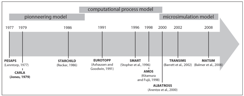
Figure 1.
Evolution of activity based models through time.
The pioneering model was developed from 1970 to 1990. Bo Lenntorp [5] was the first to operationalize the time geographical framework by developing a model (PESAPS) designed to calculate individual space time paths corresponding to specific activity programs. CARLA [6] and later STARCHILD [7] were inspired by this precursory model and are considered as the first operational activity based model, even though they were developed mainly for research purposes and not for any operational application.
The second period corresponds to the first implementation of computational process models from 1990 to 2000 [8]. More sophisticated models were designed to manage activities land use and vehicle transaction components [9,10]. AMOS [11] was the first model applied in Washington DC for studying travel demand management policies. The second emblematic model of this period is ALBATROSS [12] (A Learning-Based TRansportation Oriented Simulation System). This system relies on the following principle: individual entities modeled are following a computational process to build and achieve their daily program, based on activity space that is limited by constraints, defined by Hägerstrand [2]. Mc Nally et al. [3] consider ALBATROSS as “a significant contribution to the state of the art and its on-going development continues to influence other activity-based approaches”. Despite this influence, the computational process model is limited by an important complexity due to its holistic structure.
The last period (2000–2015) reflects the need to introduce more dynamics grounded in behavioral representations in those microsimulation models. The recent contributions of artificial intelligence, in particular agent based models and Cellular automatas contributed to renew the methodological framework of urban geosimulation field [13]. Along this way, TRANSIMS [14] is certainly the most significant activity based model. Developed by the Los Alamos national Laboratories for the US Department of Transport, Transims is a modular approach mainly composed of a synthetic generator of population, constructed with census population and household survey. However, the rigidity of the relation between the different components and the importance of the data collection phase make difficult applying Transims to real case studies. More recently, the somewhat upgraded generic structure of MATSIM [15] gave more flexibility, leading to various policy oriented applications around the world, for example with the even more traffic evolution adapted micro-simulator TransMob [16].
According to Mc Nally et al. [3], the next step for microsimulation model in the short term is to give an operational status. In this way, the MIRO approach suggests building the foundation of a 3A approach Agent-Activity-Actors model:
- Agent to introduce individual behavior;
- Activity in order to address a schedule and trip;
- Actors to consider policy for forecasting real case studies.
2.2. The MIRO Approach
MIRO relies mainly on the concept of “situated agents”, a computer science anchorage that shares analogies with what may be called “geographic agents”. According to [17], situated agents may be seen as autonomous entities defined by: (i) their location in a given environment (often defined as a geometric or geographic space.); (ii) their-body-(a representation of themselves); (iii) a survival or satisfaction function, driving their behavior; (iv) their capacity to perceive and explore their environment and modify it according to limited skills. Generally speaking, two main categories of Agent-Based Models, or “ABM”, relying on situated agents can be identified: on the one hand ABM in which agent behaviour is impacted by their environment, often through a stimulus-response process and on the other hand ABM in which agents try to achieve scheduled tasks [18]. However, these two different approaches rarely consider time as a limited resource: the temporal dimension is often introduced simply as a simulation step, and not that often as a limiting factor, that will force the agent to re-organize its scheduled tasks to fit in the simulation time. Nevertheless, when it comes to the exploration of daily movements in modern cities, one may wonder whether this limited spatio-temporal vision is adapted to the problem at hand. Therefore, in MIRO, we define agents being both spatially and temporally situated and having very specialised capacities linked to the combination of these two fundamental dimensions (Figure 2).
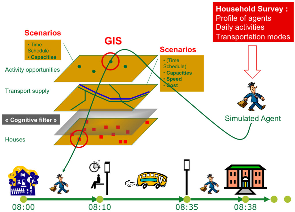
Figure 2.
Characteristics and goals of geographic agents in MIRO.
Generated from real data in order to be representative of the population under study—and thus constituting a so-called “synthetic population”—our agents are assigned, among other characteristics, a list of daily activities, as well as fixed home and work places. Their objective, during a given simulation, is therefore to organize, schedule and carry out their activities, taking into account constraints imposed by their environment, including the ones emerging from other agents’ behaviors (road traffic, for example). This last point is of crucial importance as it raises the question of the possible dynamic adaptation of agents, facing unusual traffic conditions for example. Furthermore, being reactive by essence, our agents may also, under certain conditions, act as cognitive agents, able to learn from past situations and to adapt their upcoming choices. However, such evolutions, while seeming reasonable and logically grounded, lead to a significant increase in complexity as agents may diverge very clearly, leading to a rapid increase in heterogeneity. Such an increase in complexity has a price, as our capacity to understand the behavior of the model is directly connected to its complexity. Therefore, we decided to control such potential inflation as much as we could and to focus primarily on non-adaptive agents. Due to the interdisciplinary context of the projet, the platform GAMA that we chose is suitable because contrary to Netlogo, GAMA permits to run large scale simulation and support natively GIS. Concerning frameworks such as Repast or Mason, Gama is based to a stakeholders oriented language that facilitate exchange between participants of the project while performances are quite similar.
3. Defining a Virtual City
Being applied as a case study to the french city of Grenoble (160,000 inhabitants), the model requires us to create a virtual city as much empirically grounded as possible, taking into account multi-sources data, being whether spatial (urban ressources), temporal (opening hours of the urban resources) or related to the inhabitants characteristics and their daily patterns of activities. To do so, we deal with several databases and surveys and call on various statistical methods.
3.1. Constitution of the Spatio-Temporal Database of Opening Hours of Grenoble Urban Resources
The model developed relies on a spatio-temporal database detailing the location as well as the opening and closing hours of urban resources, defined here as the set of services, shops, businesses and public institutions to which individuals move in order to achieve their daily activities. Facing the absence of such data in Grenoble (and more generally in most French cities) we have therefore developed an appropriate methodology to build the needed database.
Concerning public facilities (town hall, schools, police, etc.), the data were collected exhaustively, due to the small number of resources involved (about 900). Data were collected directly via Internet and telephone contacts.
The approach is somehow different for shops, services and businesses. We decided to complete a database bought from the Chambre de Commerces et d’Industrie (CCI for Chamber of Commerce and Industry). This database describes all shops, services and businesses in terms of its activity category, number of employees, location, etc., of a given area. To complete this existing database, the following diagram illustrates the overall methodology we developed (Figure 3).
First, the resources from the CCI database were ordered by their “APE”, or “main activity code”, which is a classification of the building main activity. All the resources were then geolocated using MapInfo and ArcGIS softwares, plus Google Maps database. In total, 97% of resources were located with sufficient accuracy.
To assign the opening and closing hours for shops, services and businesses, a telephone survey was carried out. Given the large number of resources in the 26 municipalities of the study area, a sample (14,451) was selected. The proportional stratified random sampling method was applied. This method consists in dividing the study population into subpopulations and selecting independent samples within each stratum using the same sampling rate. The sampling criteria that were taken into account are the activity type and the density of resources for shops and services, as well as the activity type and the number of employees for companies. In total, 12% of shops and services and 9% of companies were surveyed.
Once the opening hours were collected for the samples, we generalized them to the remaining population taking into account the type of activity and the density of resources within the area. For that purpose, a Python script was developed. It applied opening hours to each resource that had not been surveyed depending on its type of activity and the local density of resources. This database is an important input of the model as is constitutes the environment in which the agents, once generated as a synthetic population, will apply their schedule.
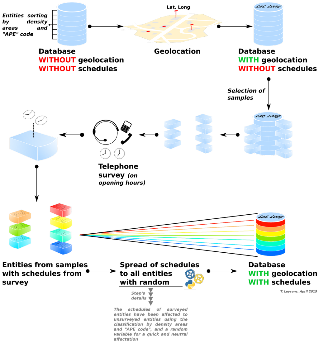
Figure 3.
Methodology to constitute our spatio-temporal database of opening hours of urban resources.
3.2. Generating the Synthetic Population
3.2.1. Survey Data as an Input
In order to create a model based on observed daily mobility, one of the most thorough dataset available in France is the "Enquête Ménages-Déplacement", or "EMD" (household travel survey). This standardized survey is focused on the daily mobility in large urban districts.
The data production draws upon questionnaires given to randomly-selected households inside specific representative zones of the urban area, between the end of November 2009 and beginning of April 2010, excluding holidays and weekends. The collected data are focused on the day preceding the survey for each individual, and cover a 24 h period, in which every journey must be as detailed as possible in space and time.
The 2010 EMD survey used in this work collected 7600 households from Grenoble’s urban area in 97 districts, which means around 16,000 people aged 5 years and over.
We elaborated a typology of the population according to their socio-economic and demographic characteristics. The statistical aggregation method also keeps the groups different enough in their characteristics and numbers (Table 1).

Table 1.
Typology of population according to their socio-economic, demographic characteristics and daily activities.
| Category | Headcount |
|---|---|
| 1: Active people | 3914 |
| 2: Single mothers/Part-time workers | 1313 |
| 3: Unemployed | 577 |
| 4: Active and unemployed 40–64 years old people | 2706 |
| 5: Students | 1283 |
| 6: Retired people | 2131 |
| 7: Young people (going to school) | 2897 |
3.2.2. Data Process and Validation of the Results
Based on these categories, a synthetic population could be generated following four important steps: (i) definition of attributes that will be assigned to agents; (ii) generation of agents under constraints of attributes using GenStar (Gen*) prototype [19]; (iii) validation of the population obtained; (iv) spatial allocation of agents created.
The following table (Table 2) illustrates the chosen attributes to be assigned.

Table 2.
Attributes assigned to the synthetic population.
| Attribute | Dependencies | Levels |
|---|---|---|
| Category | age | [1,2,3,4,5,6,7] |
| Age | category | 5:17, 18:24, 25:34, 35:49, 50:64, 65:100 |
| Gender | category | man, woman |
| Area | category | One of the 97 area |
| Main Activity | category | Work, Study, Shopping, etc. (8 possibilities) |
| Vehicle type | age, area | No vehicle, authorized vehicle (registred after 2001), un authorized vehicle (registred before 2001) |
The synthetic population is then generated with the Gen* algorithm [19], using a learning sample of the initial survey data. The frequency of each desired attribute is extracted from the survey, with its dependency to an other attribute. The Table 3 below gives an example of the frequency of people from the survey who are male (Gender = 1) depending on their category (from 0 to 2 in the example). Gen* will use such inputs to generate a conditional probability law for every attributes.
Therefore, empirical probability laws for every attribute and its dependencies (conditional probabilities) can be generated, as the basis of a statistically coherent synthetic population.
Then, the validation procedure per se follows three steps.
Firstly, we use 10 random subsets—called learning sets—extracted from a percentage of the individuals of the EMD survey, in order to generate a synthetic population with Gen*. Then we compare these subsets with the rest of the population, which is the validation set (Figure 4).

Table 3.
Example of conditional probability law for male agents.
| Category | Gender | Frequency |
|---|---|---|
| 0 | 1 | 1992 |
| 1 | 1 | 183 |
| 2 | 1 | 273 |
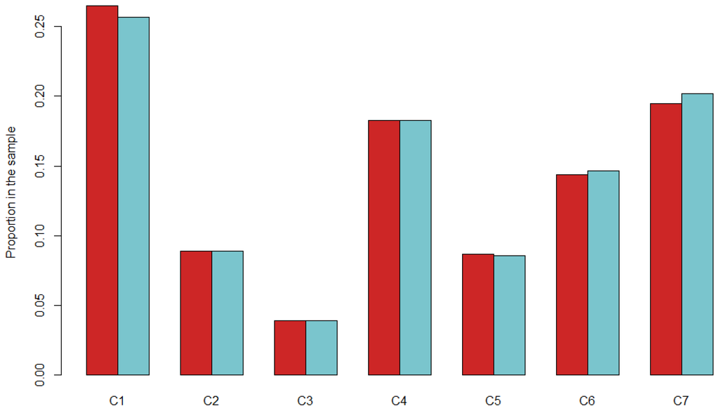
Figure 4.
Difference in categories’ proportions between 90% and 10% learning sets.
Secondly, we average the attributes of the generated population and the subsets. We compare them.
Thirdly, we compute relative errors between the learning subset and the synthetic population (Table 4).

Table 4.
Relative errors for the main attributes.
| Attribute | Value | Relative Error |
|---|---|---|
| Category | 0 | 0.007 |
| 1 | 0.012 | |
| 2 | 0.008 | |
| 3 | 0.006 | |
| 4 | 0.016 | |
| 5 | 0.002 | |
| 6 | 0.001 | |
| Gender | Man | 0.001 |
| Woman | 0.001 | |
| Age groups | [5;17] | 0.001 |
| [18;24] | 0.011 | |
| [25;34] | 0.001 | |
| [35;49] | 0.011 | |
| [50;64] | 0.006 | |
| [65+] | 0.002 | |
| Area | [100;199] | 0.002 |
| [200;299] | 0.011 | |
| [300;399] | 0.004 | |
| [400;499] | 0.008 | |
| [500;599] | 0.005 | |
| [600;699] | 0.019 | |
| [700;799] | 0.036 | |
| [800;899] | 0.013 | |
| [900;999] | 0.006 |
Even if the learning subset is around 50%, the relative error is globally under 5%, and the methodology used does not produce any incoherent combination of attributes, as soon as the frequency is equal to 0 in the input file.
Other attributes that are not shown here are aggregated values from the global survey, and cannot be specific to a subset of the population. They are nonetheless well distributed as well.
3.2.3. Localization of Agents
Once generated, agents are randomly allocated to a living place—under constraints of capacity—within the zone they belong to. Then, a working (or their other main activity) place is assigned as well, but without restriction on the zone.
To simplify the model, there is no affectation of agents to households yet. This means that agents are randomly located in buildings together. The diversity of people at the building’s scale is expected to offset the lack of details at the households scale.
Moreover, as survey data cover a much larger area (urban area of Grenoble) than our limited case study does, we made sure to take into account populations coming from external areas, allocating them as agents to a limited number of “access points” localised on the main road axis of the urban system (Figure 5).
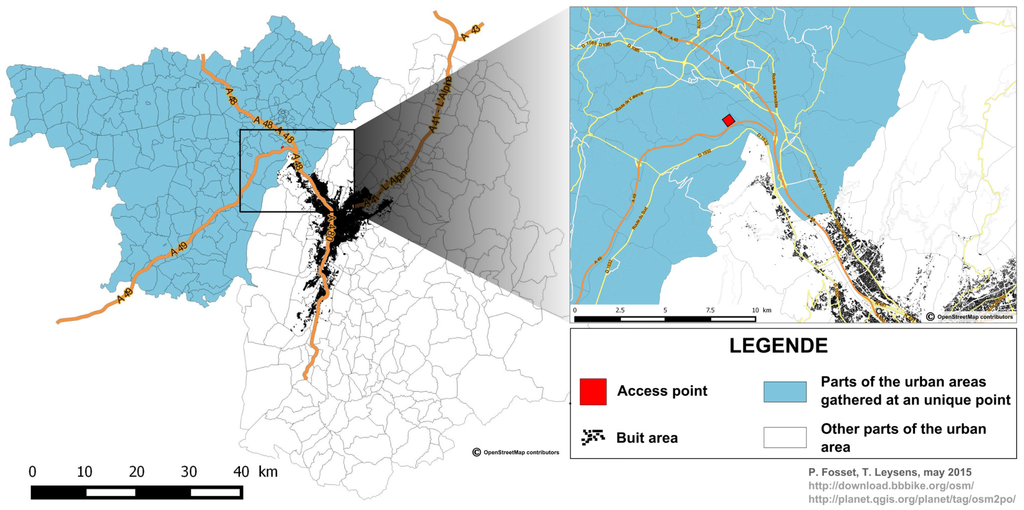
Figure 5.
Concentrating external areas in one point.
3.2.4. Generation of Agent’s Schedule
Once created, each agent picks-up a schedule in a predefined library of schedules (Table 5).
The predefined library of schedule, is derived from the full sets of combinations revealed by the EMD survey. A Python program, has been developed in order to create a set of around 5000 possible combinations of activities, according to the EMD survey.
At first, the logical combinations of all activities are generated, under the following list of constraints: existence of minimum (1) and a maximum (3) number of activities in a day; necessity for schedules to begin and end at “Home”; absence of redundancy for “Home”. These conditions are based on the analysis of the survey, revealing that the part of the population concerned by a schedule with more than three daily activities is not significant. Indeed, in every category except from the single women and partial time workers, it represents less than 2% of the combinations.
All the remaining logical combinations are sorted by main activity in a csv file, from which the schedules will be chosen and scheduled.
Several steps are implied at this level, to schedule the previously-selected schedules.

Table 5.
Schedule library extract (person #0, Main activity “Work”, time in second).
| ID_Pers | ID_Schedule | ID_ACT | ACTIVITY | DATE_BEGINNING | DATE_ENDING |
|---|---|---|---|---|---|
| 0 | 0 | 0 | Home | 0 | 49,440 |
| 0 | 0 | 1 | Work | 49,500 | 62,233 |
| 0 | 0 | 2 | Sport | 62,533 | 65,206 |
| 0 | 0 | 3 | Work | 65,326 | 78,059 |
| 0 | 0 | 4 | Home | 78,119 | 86,400 |
| 0 | 0 | 0 | Home | 0 | 29,091 |
| 0 | 0 | 1 | Study | 29,151 | 33,701 |
| 0 | 0 | 2 | Work | 33,881 | 60,751 |
| 0 | 0 | 3 | Study | 60,931 | 74,579 |
| 0 | 0 | 4 | Home | 74,369 | 86,400 |
First, we assign a main activity to each agent, according to his category and the occurrence of each activity in the schedules (provided that it exceeds 10%) from the survey.
Second, we assign the living place and main activity place to each agent, then using the library of schedules, we propose a limited number of schedules to each agent, in order to keep the choice at a realistic scale [20].
This choice is limited by the main activity that must appear in the list of activity of the schedule. We propose 10 schedules that are randomly chosen in the library.
Agents will choose a schedule in this set using utility functions (see Section 3.2.2). The parameters taken into account are: the proposed activities, the matching between these activities and agent’s category but also the time needed to reach and achieve these activities (see Section 3.2.5). Based on this, we construct a time sorted schedule with, for each activity, a beginning and an ending date (Figure 6).
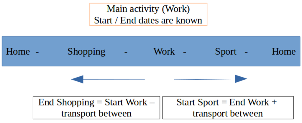
Figure 6.
Schedule creation.
We first determine the duration of the main activity, based on the mean value depending on the category. Then, we determine a time interval during the day, based on the building’s schedule concerned by the main activity and on its duration. From this duration, we randomly assign a beginning date within the interval.
From this main activity starting date, we calculate the schedules for the activities that come after and before, by subtracting the mean transportation time (always depending on categories) between them, and taking the mean time of each one as a duration. We do so, until we reach the first and last activities of the schedule.
Transportation durations and main activity durations are based on average durations from the EMD survey, and are specific to each category. The durations follow a normal distribution.
For other activities, including the time spent at home, the mean time is also used, but the proportion of the day each activity covers is calculated in order to make the durations are realistic.
3.2.5. Utility Function and Decision Process
Each agent faces distinct schedules that are theoretically feasible and mutually exclusive (representative activity patterns). Decision process is then formalised with discrete choice models that are appropriate to bring out individuals’ preferences under the assumption of rational behaviour. The goal of these models is to understand, in a somewhat causal approach, the factors that lead to individual choices in various contexts. These factors are introduced in a utility function that is supposed to “explain” the choices made and that summarises agents’ preferences.
The most widely used discrete choice model is the logit model decomposed into representative and unobserved utility [21]. In a choice set, each alternative could provide a certain level of utility for the agent. The utility that decision maker n obtains from alternative i is determined by its attributes k (representative utility). Unobserved factors related to strictly individual preferences can be added as a random term Euro (unobserved utility). However, in the logit model, this random term is assumed to be identically distributed among individuals, which is relatively consistent with the definition of our seven homogeneous groups (Table 1). This assumption is restrictive but provides a convenient and easily interpretable expression for choice probabilities.
Although more complicated expressions are possible, representative utility functions are usually formulated as a linear additive function of attributes chosen by the modeller. The utility is defined as Equation (1).
where is a vector of coefficients allocated to the potential explanatory variables .
The data source for the calculation of the discrete choice parameters is the French “Enquête Mênages Dêplacements”. Variables tested in the model are duration and travel time associated to various out-of-home activities. The utility of a schedule (or an activity pattern) is comprised of the utilities of time spent in each out-of-home activities (positive coefficient expected) and travel time from the location of an activity to another one (negative coefficient expected).
Under the principle of utility maximization, the decision maker is expected to choose the alternative that provides him the largest utility among a reduced choice set. However, the agent’s choices are not strictly deterministic and the behavioral process is based on probabilities estimation. We can define the choice probability of each activity pattern evaluated by the agent. The probability that an agent chooses an alternative is simply a function of its representative utility into the set of all evaluated activity programs . This probability is expressed as Equation (2).
Although, the probabilities of choice are distributed in a disaggregate way, according to the utilities calculated for each individual [22], the outcomes of the logit model provides an approximation of groups preferences that lead to activity program choice.
The calibration of the model is based on a selection of significant variables for which parameters are determined with the maximum likelihood method [23]. The variables are considered statistically significant if their p value remains lower than 0.05. Only significant variables are shown in the following outcomes (Table 6, with the following symbols for the corresponding p values : * p < 0.05, ** p < 0.01, *** p < 0.001).
Results show a classical strategy of maximization of several activity-times with a travel-time minimization. Travel time is not as frequently significant as expected but note that time spent in transport reduces the amount of time available for time activity.

Table 6.
Utility functions for different activities and population categories.
| Active People | Single Mothers/Part-Time Workers | Unemployed | Active and Unemployed 50–64 Years Old People | Students | Retired People | Young People (Going to School) | |
|---|---|---|---|---|---|---|---|
| Working time | 0.584*** | 0.358*** | 0.312*** | 0.152*** | |||
| Travel time to work | |||||||
| Study time | 0.118*** | 0.135*** | |||||
| Travel time to place of study | −0.124*** | −0.166*** | |||||
| Purshasing time | 1.36** | 5.12*** | 2.18*** | 0.236*** | 2.26** | ||
| Travel time to purshase | −0.242*** | −0.257*** | −0.286*** | −0.127*** | |||
| Health time | 0.811*** | 0.5*** | |||||
| Travel time to health facilities | −0.167*** | −0.268*** | |||||
| Administrative procedures time | 0.307*** | ||||||
| Travel time to administrative procedures | −0.303*** | ||||||
| Leisure time | 1.77*** | 2.0*** | 3.16*** | 6.18*** | 0.313*** | 2.13*** | 0.39*** |
| Travel time to leisure activity | |||||||
| Accompanying time | 2.58*** | 4.0*** | 4.48*** | 0.25* | |||
| Lunch time | −0.191*** | 0.231*** | |||||
| Travel time to lunch | −0.078 | −0.087 |
The outcomes of the modelling that is the final form of the utility function synthesizes groups’ preferences that will be used in the simulation. Thus, utility functions are used by agents, according to their group assignment, to choose an activity and travel time schedule in a choice set. From this point, agents expect a certain level of utility from the chosen alternative and compare it with the utility really obtained in the simulation (satisfaction measure).
These functions can capture tradeoff or compromise effects between time spent on several specific activities and travel time to reach activities localizations. That is the same level of utility can be reached with different activity programs in term of activities chosen, location and mobility behaviour. This ensures a wide range of agents behaviour.
The level of satisfaction is calculated from the utility function. If the satisfaction obtained into the simulation is below the expected one from a certain threshold level, agents can change their route, modal choice or the location of their activities before choosing a new schedule available in the library. The real utility of this new schedule should be comprised between its expected utility and the expected utility of the previous schedule chosen.
4. The GaMiroD Model
4.1. Model Composition
GaMiroD model holds a specific architecture, grounded in the various data available in Grenoble. It has been developed with the GAMA framework [24,25]. In this model, inhabitants, buildings, roads, traffic and transportation system are therefore the main dimensions we retained, following the multi-layer structure suggested in Figure 2.
Four agent species are specified:
- “Inhabitants” represent people living in the city and moving along the day to achieve their scheduled activities. The population of “inhabitant” agents is initialized following the synthetic population generation process described in previous sections.
- “Buildings” (~70,000 elements) are generated as agents from a shape file, identifying for each building in Grenoble the main associated services with their opening and closing times.
- “Stations” corresponds to the whole set of bus stations (750 in Grenoble), defined as agents holding informations regarding bus lines and their time schedules.
- “Roads” agents (~80,000) are defined by their capacity, speed limitation, and number of lanes. They are organised as a street network from which travelling paths can be computed.
For a standard simulation, nearly 550,000 active agents interact (400,000 inhabitant agents, 70,000 building agents, 750 bus station agents and 80,000 road agents). They evolve according to their own characteristics and their own behavior, both formalized by a design model.
4.2. Design Model
The designed model aims at determining the architecture of the multi-agent system. Thus, it displays agents’ species, their characteristics, their belief, their resources and their behavior, as well as possible interactions between agents. The model is presented in the Figure 7.
4.2.1. A Descriptive Multi-Agent-System Based on Data
The GaMiroD model integrates four species of situated agents (Inhabitants, Stations, Buildings and Roads) extracted from data of the city. These agents belong themselves to two categories: moving agents and fixed agents. Fixed agents (i.e., Station, Building and Road species) describe the urban environment whereas moving agents (i.e., Inhabitant specie) represent individuals evolving within the city along the day.
Whatever their specy, agents are defined by characteristics and behaviors. Agents’ attributes determine an internal state agents expose (+) or hide (−) to others. For example, a building agent may be an urban service such as a workplace, a restaurant and so on. It holds four characteristics: an identification key (id); a service type (usage—e.g., “workplace”, “restaurant”, “home” and so on); an opening state (is_open); an opening timetable (open_at—a set of one to three opening slots). In this example, usage, opening state and opening timetable are exposed to other agents whereas the identifying key is hidden.
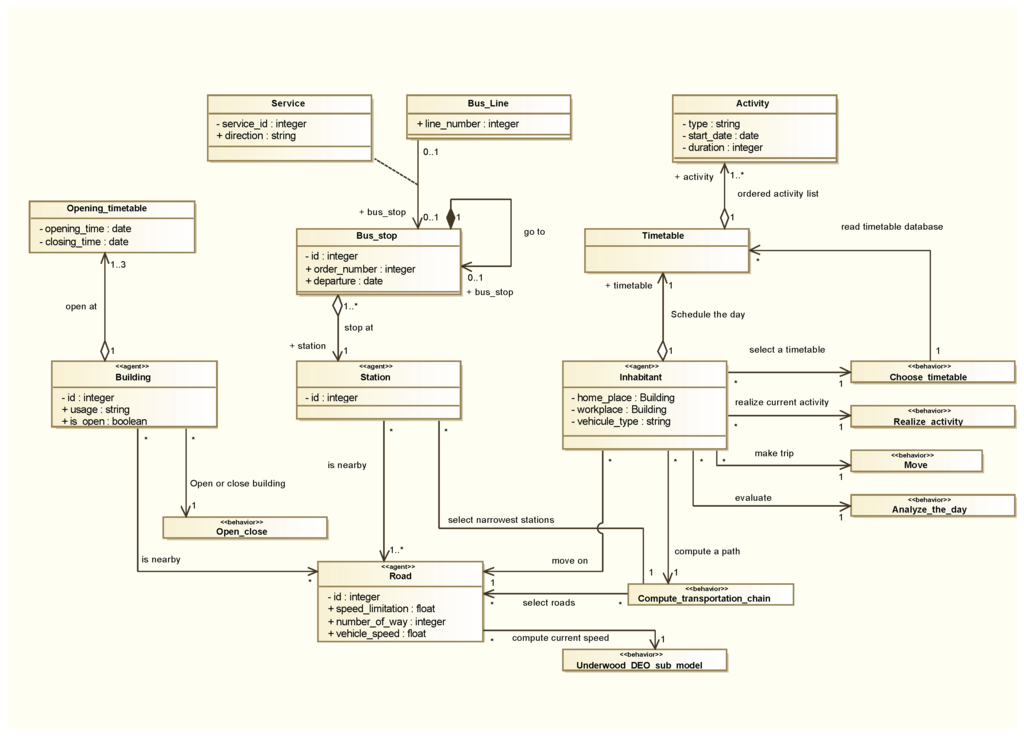
Figure 7.
Design model of the multi-agent system.
4.2.2. A Highly Dynamic Multi-Agent System
GaMiroD assumes cities are highly dynamical systems, among which inhabitants are evolving and interacting with their environment as well with each other. For that reason, fixed agents composing the environment of the MAS (Building, Station and Road) and moving agents (Inhabitant) hold specific behaviors.
Building and station behaviors are quite deterministic. For the former, the “Open_close” behavior modifies the state of the agent (attribute “isOpen”) according to the time of the day and the agent timetable. For the latter, Station agents compute the transportation duration between two stations (from the departure to the arrival). This behavior is based on an evolution of Dijkstra algorithm that takes into account transportation timetable, transfer between two correspondences, and traffic congestion. Therefore, public transport is defined as a network of stations constrained by a transportation timetable and urban traffic: No bus, nor tramways are explicitly modeled. Transportation vehicles are described through an association of Bus_line, Service and Bus_stop. A couple (Bus_line, Service) models a vehicle moving from station to station in order to pick-up and deliver people (Inhabitants). This modeling architecture has many advantages, especially to fit data we obtain from the municipality and to permit an operational assessment of public transport policies without adding too much complexity.
The behavior of Inhabitant agents is more human inspired. Their life cycle is summarized in the figure (Figure 8). According to their timetable, they move (walking, driving or by bus) in the city and achieve activities during the day. Then, agents analyse their performance of the day, evaluate their timetable and switch to a new one if necessary. Five sub behaviors lead inhabitant mobility:
- “choose_timetable” Ten timetable are associated to inhabitant during the population generation. One of them is selected according to agent state and utility function;
- “compute_transportation_chain” Before moving, each agent computes and chooses (based on the time estimation from the Dijkstra shortest path algorithm) its trip from its current location to the next activity location. Multi-modal chains are allowed, for example 3 km by car to go to the bus station, then 2 km by bus to another station and finally 500 m walking to the destination. Transportation mode choice depends on social characteristics of agents, and particularly whether they possess a car or not;
- “move” Realize the journey between two activities according to the transportation chain computed in the previous task;
- “realize_activity” Realize an activity until it is finished;
- “analyze_the_day” The timetable is achieved. Agents analyze their performance of the day and compute a satisfaction rate. They keep their current timetable if it is acceptable or select a new one if needed.
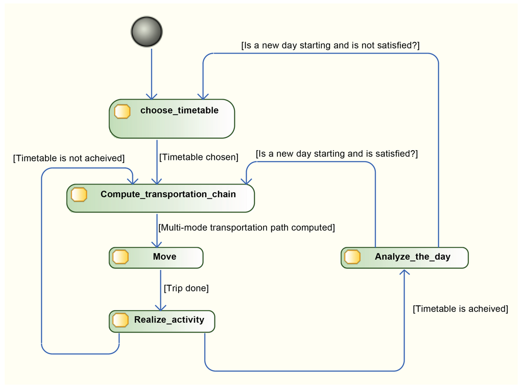
Figure 8.
Life cycle of the agents.
In this version of GaMiroD, Inhabitants do not have direct exchanges with other inhabitants to accomplish their timetable. Households are not explicitly described, but they are taken into account during population generation. Nevertheless, inhabitants interact in an indirect manner with each others when they move: they are constrained by a macro-scale traffic model.
4.2.3. A Macroscopic Traffic Model Applied at a Microscopic Level
Various traffic models are proposed in the literature and give either a micro-scale point of view of mobility (e.g., NaSch model [26]) or a macro-scale description of congestion such as LWR [27,28] or Underwood [29]. The former model describes vehicles as individuals, able to accelerate or decelerate according to road speed limitation but also speed of next vehicle ahead. The latter models the traffic as a flux of individuals and outlines speed variation using macroscopic differential equations.
GaMiroD adopts a hybrid approach associating Underwood macro-scale model with an individual centered mobility model. This approach allows us to keep a fair resolution for traffic at road scale without introducing increasing too much behavioral complexity, especially within the “moving” and “compute_transportation_chain” steps.
As described in previous paragraphs, the road network is stored as a graph composed of nodes (junctions) and edges (sections). Each edge is valued by a maximum speed (speed limitation), a width (number of lanes) and a length. The speed of moving agents depends on their transportation mode, i.e., fixed for pedestrians (5 km/h) or constrained by traffic model for cars and buses. The speed of vehicles is also updated during the simulation according to the deterministic Single-Regime Speed-Density Underwood model presented by Equation (3).
With:
- the speed of vehicles driving on edge i;
- the free-flow speed (speed limitation) of edge i;
- the maximum traffic capacity of edge i, that takes into account the number of lanes and the length;
- the number of vehicles driving of edge i, and
- α a congestion impact factor.
Given the capacity of the edge, its capacity and the number of vehicles located on it, the Underwood model allows us to compute an instantaneous speed for each vehicle.
4.2.4. The Particulate Matter (PM10) Emission
Directly related to the traffic model is the particle emission rate per vehicle. We grounded the estimation of emission on the EU-classification of vehicles which correspond to six emission levels: passenger vehicles (1400-2000 cc, diesel) constructed after july 1993 obey Euro1 standards and the most recent constructed after september 2015 respond to Euro VI standards. We used here a simple polynomial law of degree six [30] depending on the speed and type of vehicle. This law is coefficient-specific for every type of vehicle between the Euro 1 and Euro 6 classification. We applied the Euro 1 coefficients for the “non ecological” cars, and the Euro 6 for the “ecological” ones. The polynomial law is estimated at every step for each vehicle, using the coefficient of either Euro I or Euro V. Particles accumulate directly on the road where they are emitted, at every step and for every agent in a car. These data are the ones saved in the output, in order to observe the impact of the traffic depending on the type of vehicle possessed.
5. Simulation and Results
Urban authorities are facing the challenge to reduce the impacts of urban traffic on outdoor air pollution. For over two decades, the impacts of air pollution on urban residents health has been proven and lead to several recommendations from the World Health Organization (WHO) that are regularly reminded. In May 2014, WHO-media center news release warn that “Air quality in most cities worldwide that monitor outdoor (ambient) air pollution fails to meet WHO guidelines for safe levels, putting people at additional risk of respiratory disease and other health problems” [31]. In this context, European authorities are promoting urban policies targeting air pollution. Thus, many cities in Europe put in place measures such as Low Emission Zone–LEZ–in English, or Zone d’Actions Prioritaires pour l’Air–ZAPA–in French , traffic limited zones or city tolls, in order to reduce traffic pollution and to improve air quality. However, it is still a critical issue for the local authorities to manage to prohibit—in a certain extend area and for certain type of vehicles—individual mobility while maintaining an equitable individual access to the city. Charleux [32] demonstrates that putting in place a LEZ area in Grenoble would have a socially differentiated impact on people’s mobility. In this paper, the analysis is grounded on Household Travel Survey data that describe a representative sample of daily trip-chaining for each person interviewed. It permits to evaluate not only who and how many people would be affected by a LEZ area, but also how these people would adapt their behavior within the new context in terms of modal choice, new itineraries and eventually new activities. It could not either simulate the effect of traffic reducing on vehicles emission and air quality.
That is why we build here a scenario applied to an LEZ area in the center of Grenoble city (based on a real ZAPA which was projected by the local authorities). We use GaMiroD to simulate:
- in which extent the LEZ area impact the traffic and the air quality in the different zones of the city;
- how the population will be impacted considering their capacity to maintain their daily programs and mobility.
Figure 9 shows the simulated impact of the introduction of an LEZ in Grenoble city center on automobile traffic. Major traffic reports occur—as expected—on the major bypass axes but not only. Main roads may be used to bypass the city center for those who cannot drive there while, in the same time, secondary roads are impacted by evolutions in activity places chosen by agents, due to LEZ constraint.
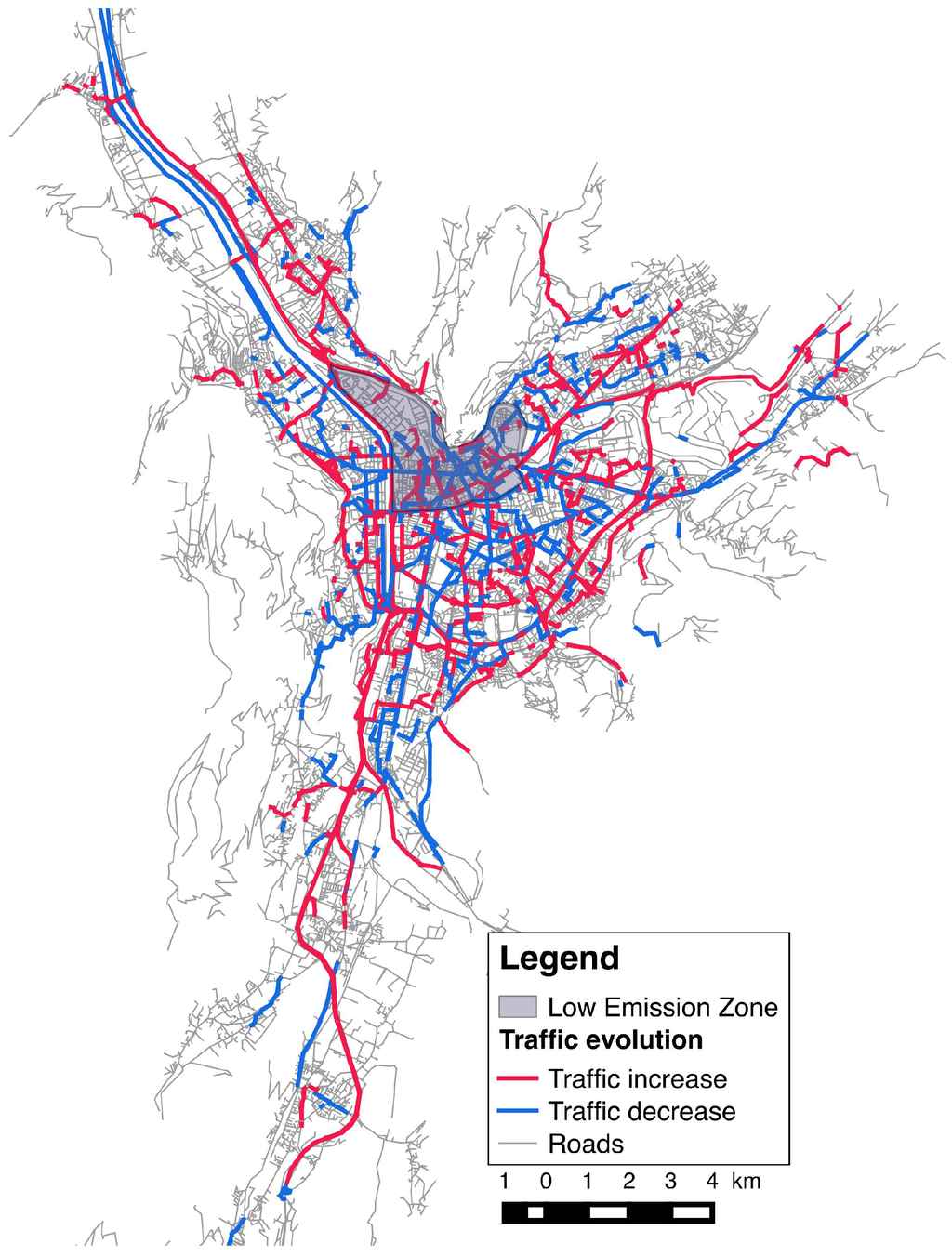
Figure 9.
Simulation of the LEZ impact on the car traffic in Grenoble (100,000 agents).
Moreover, mapping of particulate emissions (PM10) associated with the introduction of LEZ (Figure 10) reveals a significant improvement in air quality within the ZAPA is offset by an equally significant degradation of the quality of the air in other areas, because of the postponement of traffic and/or activities generated by the introduction of LEZ.
The calculation of losses and gains throughout the area shows that the global impact of LZ on the amount of PM10 emission is negative: the average rate of change between the situations with and without LEZ weighted by the resident population per area is thus −8.3%, showing an overall increase in exposure of resident populations to PM10. The small size of LEZ and its central location are probably of concern and the interest of this approach is to explore other alternative scenarios, without these possible negative effects.
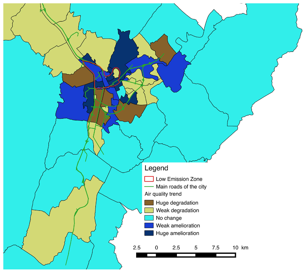
Figure 10.
Impact of the LEZ on the city districts air quality.
Another benefit of such individual-based approach is to lead assessment at that level of detail. It is thus possible to identify for example every agents whose schedule is affected by the introduction of LEZ. Figure 11 shows the location of these agents (places of residence). Note that a very large area around LEZ is concerned (the entry points of the city being penalized significantly) and the impact on activity chains is systematically negative, revealing the negative impact of LEZ in terms of accessibility to the city and its resources. Its location in the heart of Grenoble monocentric urban system structurally amplifies this phenomenon.
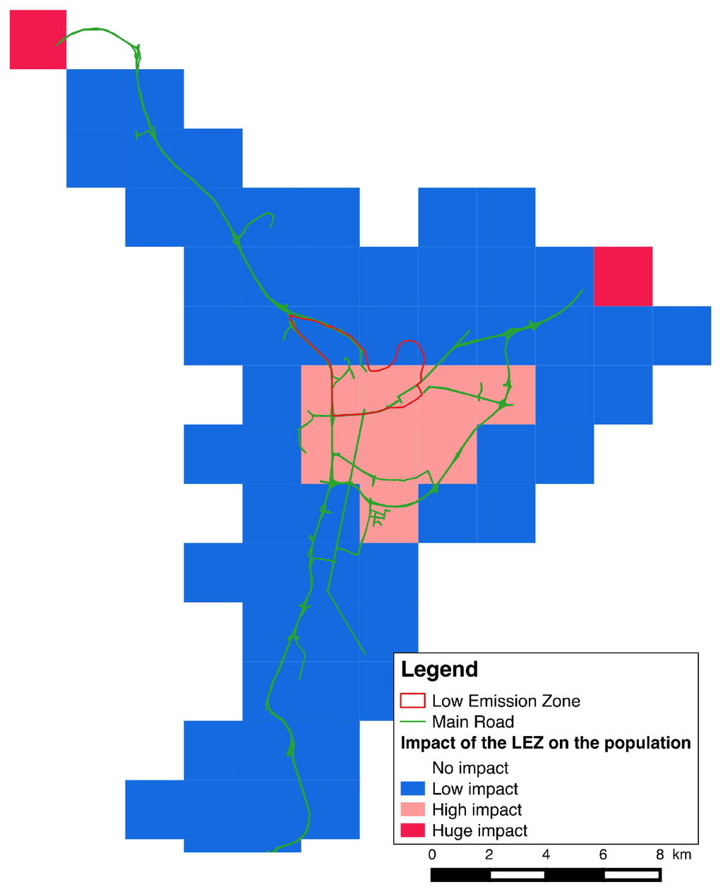
Figure 11.
Global impact of the LEZ on the population.
6. Conclusions
Modeling and simulation of urban daily mobility takes its roots in several scientific areas, from transportation sciences, social and economic sciences, operational research, mathematics and computer sciences. Agent based modeling offers new insights and possibilities in this perspective, due to a strong analogy between the concepts of situated and geographic agents. Moreover, due to technological evolutions (including soft and hardware) as well as increasing data availability, large scale computations are more than ever at our fingertips.
Today, our model is focusing on LEZ impact on pollution and population. Yet, the GaMiroD could investigate various problems, especially the ones on which urban daily dynamics have a major impact. Its large application domain and the possibility to simulate french middle size town at their real scale allow us to consider the GaMiroD model as a city laboratory which permits us to try, test and evaluate, in silico urban planning or technological novelty. For instance, it is both possible to simulate a traffic management plan and evaluate smart cities’ novelty (intelligent signalisation, connected vehicles). The GaMiroD model could help in decision making. Nevertheless, the model should evolve in several ways, especially in its performance to support large towns and southern towns, and its usability to be appropriated by stakeholders. In the first case, research in high performance computing should be conducted. For the second point, the model should be applied to a new case study in order to give us enough experience to design an efficient and stakeholder-oriented simulator.
Acknowledgments
The MIRO project was funded successively by PREDIT3 (contract MT 03MT66, scientific coordinator Christophe Lang), by the french National Agency for Research (contract ANR-08-VD-00, scientific coordinator Arnaud Banos) and the French Ministry of Ecology, Sustainable Development and Energy (contract 13-MT-GO6-8-CVS-038 2013, scientific coordinator Arnaud Banos).
Author Contributions
Every author equally contributed to the reported work. Moreover, Pierre Fosset, coordinated the whole process.
Conflicts of Interest
The authors declare no conflict of interest.
References
- Chapin, F.S. Human Activity Patterns in the City: Things People Do in Time and in Space; John Wiley & Sons: New York, NY, USA, 1974; p. 272. [Google Scholar]
- Hägerstrand, T. What about people in regional science? Pap. Reg. Sci. Assoc. 1970, 24, 7–21. [Google Scholar] [CrossRef]
- Nally Mc, M.G.; Rindt, C. The Activity-Based Approach. In Handbook of Transport Modelling, 2nd ed.; Elsevier: London, UK, 2008. [Google Scholar]
- Greaves, S.; Stopher, P. A Synthesis of GIS and Activity-Based Travel-Forecasting. Geogr. Syst. 1998, 5, 59–90. [Google Scholar]
- Lenntorp, B. Paths in space-time environments: A time geographic study of movement possibilities of indviduals. Environ. Plan. A 1977, 9, 961–972. [Google Scholar]
- Jones, P.M. New Approaches to Understanding Travel Behaviour: The Human Activity Approach; Redwood Burn Ltd.: London, UK, 1979; pp. 55–80. [Google Scholar]
- Recker, M.G. A Model of Complex Travel Behavior: Part I—Theoretical Development. Transp. Res. A Gen. 1986, 20, 307–318. [Google Scholar] [CrossRef]
- Gärling, T.; Kwan, M.-P.; Golledge, R. Computational process modeling of household activity scheduling. Trans. Res. B 1994, 28, 355–364. [Google Scholar] [CrossRef]
- Axhausen, K.W.; Goodwin, P.B. EUROTOPP, towards a Dynamic and Activity-Based Modelling Framework. Adv. Telemat. Road Transp. 1991, 2, 1020–1039. [Google Scholar]
- Stopher, P.R.; Hartgen, D.T.; Li, Y. SMART: Simulation Model for Activities, Resources and Travel. Transportation 1996, 23, 293–312. [Google Scholar] [CrossRef]
- Kitamura, R.; Fujii, S. Two Computational Process Models of Activity-Travel Behavior. In Theoretical Foundations of Travel Choice Modeling; Emerald Group Publishing Limited: Oxford, UK, 1998; pp. 251–279. [Google Scholar]
- Arentze, T.; Timmermans, H. Albatross: A Learning Based Transportation Oriented Simulation System; Eindhoven: Eirass, The Netherlands, 2000. [Google Scholar]
- Benenson, I.; Torrens, P. Geographic Automata Systems. Int. J. Geogr. Inf. Sci. 2005, 19, 385–412. [Google Scholar]
- Barrett, C.; Bisset, K.; Jacob, R.; Konjevod, G.; Marathe, M. Classical and Contemporary Shortest Path Problems in Road Networks: Implementation and Experimental Analysis of the TRANSIMS Router. In Proceedings of the Algorithms-ESA, Rome, Italy, 17–21 September 2002; pp. 313–319.
- Balmer, M.; Nagel, K.; Raney, B. Large-Scale Multi-Agent Simulations for Transportation Applications. J. Intell. Transp. Syst. 2004, 8, 205–221. [Google Scholar] [CrossRef]
- Huynh, N.; Perez, P.; Berryman, M.; Barthelemy, J. Simulating Transport and Land Use Interdependencies for Strategic Urban Planning—An Agent Based Modelling Approach. Systems 2015, 3, 177–210. [Google Scholar] [CrossRef]
- Ferber, J. Multi-Agent System: An Introduction to Distributed Artificial Intelligence; Addison Wesley Longman: Harlow, UK, 1999. [Google Scholar]
- Chu, Y.; Wassick, J.M.; You, F. Efficient scheduling method of complex batch processes with general network structure via agent-based modeling. AIChe J. 2013, 59, 2884–2906. [Google Scholar] [CrossRef]
- Irit GenStar. Available online: http://www.irit.fr/genstar/ (accessed on 14 January 2016).
- Tversky, A. Elimination by aspects: A theory of choice. Psychol. Rev. 1972, 79, 281–299. [Google Scholar] [CrossRef]
- Train, K. Discrete Choice Methods with Simulation, 2nd ed.; Cambridge University Press: Cambridge, UK, 2009. [Google Scholar]
- Ben-Akiva, M.; Bierlaire, M. Discrete choice methods and their applications to short term travel decisions. In Handbook of Transportation Science; Hall, R., Ed.; Kluwer: Boston, MA, USA, 1999; pp. 5–34. [Google Scholar]
- Ben-Akiva, M.; Lerman, S.R. Discrete Choice Analysis: Theory and Application to Travel Demand; MIT Press: Cambridge, MA, USA, 1985. [Google Scholar]
- Gama Platform on Github. Available online: https://github.com/gama-platform/gama/wiki (accessed on 14 January 2016).
- Grignard, A.; Taillandier, P.; Gaudou, B.; Vo, D.-A.; Huynh, N.-Q.; Drogoul, A. GAMA 1.6: Advancing the Art of Complex Agent-Based Modeling and Simulation. In PRIMA’2013: Principles and Practice of Multi-Agent Systems, Lecture Notes in Computer Science; Springer: Berlin Heidelberg, Germany, 2013; Volume 8291, pp. 117–131. [Google Scholar]
- Nagel, K.; Schrekenberg, M. A cellular automaton model for freeway traffic. J. Phys. I 1992, 2, 2221–2229. [Google Scholar] [CrossRef]
- Lighthill, M.J.; Whitham, G.B. On kinematic waves II: A theory of traffic flow on long, crowded roads. Proc. R. Soc. Lond. Ser. A 1955, 229, 317–345. [Google Scholar] [CrossRef]
- Richards, P.I. Shock waves on the highway. Oper. Res. 1956, 4, 42–51. [Google Scholar] [CrossRef]
- Underwood, R. Speed, Volume, and Density Relationship Quality and Theory of Trac Flow; Yale Bureau of Highway Traffic: New Haven, CT, USA, 1961. [Google Scholar]
- UK Ministry of Transport. Available online: https://www.gov.uk/government/uploads/system/uploads/attachment_data/file/4258/viewer.xls (accessed on 15 January 2016).
- WHO air quality guidelines. Available online: http://www.who.int/mediacentre/news/releases/2014/air-quality/en/ (accessed on 15 January 2016).
- Charleux, L. Contingencies of environmental justice: The case of individual mobility and Grenoble’s low-emission zone. In Urban Geography; Taylor & Francis: London, UK, 2014; pp. 1938–2847. [Google Scholar]
© 2016 by the authors; licensee MDPI, Basel, Switzerland. This article is an open access article distributed under the terms and conditions of the Creative Commons by Attribution (CC-BY) license (http://creativecommons.org/licenses/by/4.0/).