Unpacking Policy–Instrument Mixes: An Exponential Random Graph Model Analysis of China’s Urban Public Safety Policy

Highlights

How does this work link to systems science through its contributions to systems practice, theory, and/or methodology?

• Policy–instrument mixes (PIMs) can be viewed as complex systems of interacting instruments that jointly address interdependent governance tasks.
• Modeling PIMs as networks enables ERGMs to examine how instrument attributes and endogenous structures shape their formation.

What are the main findings and/or the implications of the main findings?

• Policy instruments participated unevenly, with ties concentrating around highly connected instruments that may provide stable connection points for policy adjustment.
• PIM changes broadly matched shifts in China’s urban public safety agenda, while adding more instruments did not necessarily create more extensively connected mixes.

Abstract

Urban public safety (UPS) governance depends on policy–instrument mixes (PIMs), which combine instruments to address complex and systemically interdependent public safety problems. However, researchers have paid limited attention to their formation patterns. This study examines PIM formation in China’s UPS policy across two dimensions: policy–instrument characteristics and the structural properties of the mixes. Using 13,841 instrument-containing official policy texts from 2004 to 2023, this study identifies fine-grained policy instruments using a named entity recognition (NER) model. It then constructs annual policy–instrument co-occurrence networks and combines descriptive network analysis with exponential random graph models (ERGMs). The four main findings are as follows: (1) PIM networks expanded substantially, but observed combinations continued to comprise only a small share of all possible policy–instrument pairings. (2) Policy instruments participated unevenly in PIM formation, with connections tending to concentrate around highly connected instruments. (3) Usage frequency and category homophily showed stable positive associations with PIM formation, indicating stability and focus in policy–instrument use. (4) Annual changes in PIM formation broadly corresponded with shifts in China’s UPS policy agenda, suggesting timely adjustment to changing risks and governance demands. These findings offer systems-level insights into the relational organization of PIMs in China and comparable governance contexts facing cross-sectoral public safety risks.

1. Introduction

Urban public safety (UPS) is central to safe, inclusive, resilient, and sustainable urban development [1]. It involves interdependent governance tasks spanning sectors, administrative responsibilities, and policy domains. To govern UPS, governments issue policy documents that specify policy instruments and the governing techniques used to translate public safety goals into governmental action [2]. As it is difficult to address such governance tasks through a single policy instrument, governments combine diverse policy instruments to organize risk prevention, inspection, and rectification, emergency preparedness, responsibility allocation, and public mobilization. These joint arrangements form policy–instrument mixes (PIMs), which are interacting sets of multiple policy instruments within a policy field [3]. PIMs are therefore central to understanding how complex governance tasks are organized through relations among instruments and translated into coordinated administrative arrangements.

Recent research has demonstrated the value of PIMs by examining how they are designed to pursue policy goals [4,5], how they relate to policy performance [6], and how policy actors select particular instruments [7]. However, UPS governance faces diverse and rapidly changing risks and governance tasks, often requiring many policy instruments within the same policy field. As more policy instruments are incorporated into a PIM, the number and complexity of interactions between them also increase. In order to achieve more effective UPS governance, it is therefore necessary to unpack PIMs and understand both the characteristics of the instruments involved and how they interact and are organized within the mix. This can help explain how complex PIMs are formed, how coherence within the mix is established, and how these configurations may influence policy implementation.

Considering that PIMs consist of multiple policy instruments, understanding their formation requires considering both the characteristics of individual instruments and the structural features of their interactions. At the level of policy–instrument characteristics, policy-mix research highlights trajectories and patterns of instrument use over time [4], while empirical research shows that the use and prominence of policy instruments may be uneven across policy stages [8]. Thus, it is important to identify which instruments and instrument categories repeatedly occupy prominent positions within a PIM. At the structural level, policy instruments within a PIM may reinforce one another, but their interactions may also generate tensions, inconsistencies, or counterproductive effects. Therefore, it is important to understand these interactions to maintain the coherence of the PIM and to reduce policy conflicts and inconsistencies during implementation [4,5,9]. However, how these two dimensions influence PIM formation and policy implementation remains insufficiently understood.

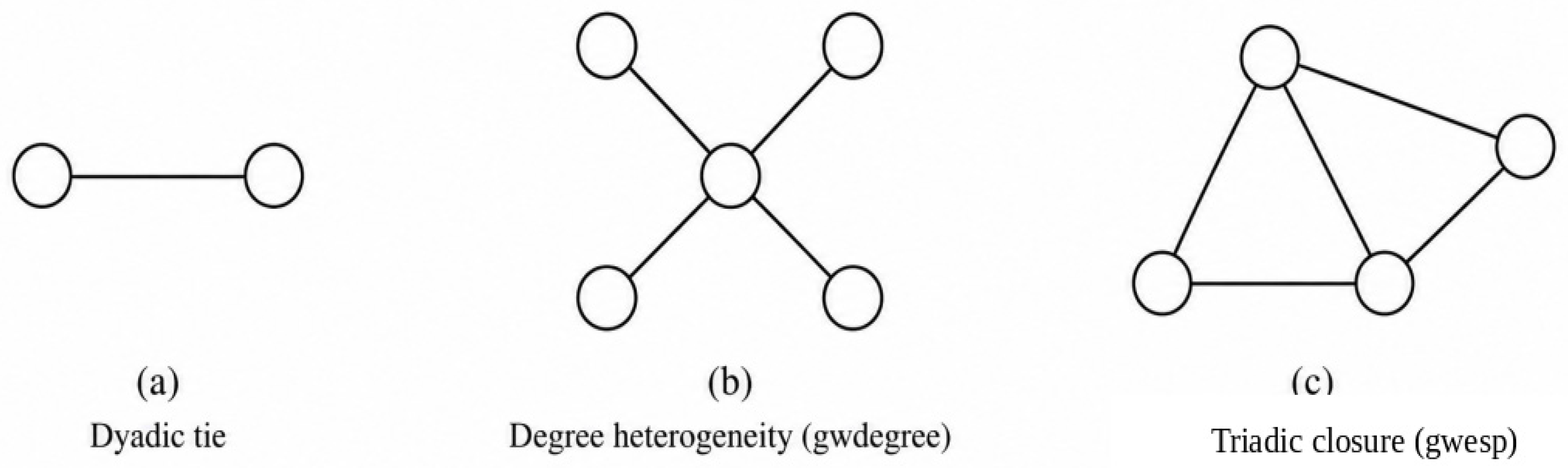
Network analysis provides a way to unpack PIMs by representing multiple policy instruments and their connections within a common system. Previous studies have used network approaches to examine interdependence among policy instruments and the coherence, synergies, and conflicts within policy mixes [7,10]. Building on this approach, this study represents PIMs as policy–instrument networks. Policy instruments are treated as nodes, and a tie is formed between two distinct instruments when they appear in the same sentence of the same policy text. Aggregating these sentence-level co-occurrence ties within each year produces a policy–instrument network, whose structural properties characterize how instruments are combined within the PIM. Exponential random graph models (ERGMs) model the probability of network ties as a function of exogenous attributes and endogenous network configurations, allowing the two dimensions identified above to be examined jointly and allowing their associations with PIM formation to be assessed [11,12]. A temporal exponential random graph model (TERGM) can also be used to analyze tie formation across repeated networks, but it is mainly designed to model temporal dependence among ties in successive networks. Because this study focuses on comparing year-specific associations under changing policy agendas instead of modeling tie persistence across years, ERGMs are estimated separately to examine how policy–instrument characteristics and endogenous network configurations are associated with PIM formation [13].

Building on this framework, this study examines how PIMs formed in China’s UPS policy from 2004 to 2023. Using 13,841 instrument-containing official policy texts, it applies a named entity recognition (NER) model to identify fine-grained policy instruments and construct annual policy–instrument co-occurrence networks. The analysis combines descriptive network analysis with ERGMs to examine six hypothesized patterns across two dimensions: policy–instrument characteristics (usage frequency, usage-frequency difference, instrument category, and category homophily) and the structural properties of the PIM (degree heterogeneity and triadic closure). The results show four main findings. First, although annual PIM networks expanded substantially, observed combinations represented only a small fraction of all possible policy–instrument pairings. This suggests that adding more instruments does not necessarily produce more extensively connected PIMs, highlighting the importance of coordination among instruments as policy responses expand. Second, highly connected instruments consistently formed combinations with low-connectivity instruments, while connections also tended to concentrate around instruments that were already highly connected. This pattern may provide stable connection points that support more flexible policy adjustment as risks and governance demands change. Third, frequently used policy instruments and instruments within the same category consistently showed a higher likelihood of being combined, suggesting stability and greater focus in PIM formation. Fourth, annual changes in PIM formation broadly corresponded with major shifts in China’s UPS policy agenda. This correspondence may indicate that policy–instrument use was adjusted in a timely manner as public safety risks and governance demands changed.

This work offers three contributions. Theoretically, it extends PIM research from describing instrument composition to examining how relations within PIMs are formed in co-occurrence networks. Methodologically, it develops a fine-grained measurement strategy that combines NER-based policy–instrument identification with network-based relational analysis, offering greater granularity than category-only or frequency-based approaches. Practically, this study provides guidance for policy formulation and policy evaluation by helping policymakers identify recurrently connected instruments, examine functionally proximate instrument combinations, and design more coherent PIMs for sustainable UPS governance in China and comparable governance contexts facing similar public safety risks.

2. Theoretical Background and Hypotheses

2.1. Policy–Instrument Characteristics and Co-Occurrence Tendencies

Existing scholarship on policy mixes has predominantly focused on the design principles and performance outcomes of instrument combinations [4,5,6], while dedicating limited attention to how instrument characteristics are associated with co-occurrence patterns. In practice, policy instruments are unevenly deployed across governance tasks and differ in their patterns of use, functional scope, and task applicability [3,8,14]. These attribute-based differences may be associated with co-occurrence patterns at both the individual and dyadic levels. Therefore, this section examines two individual-level characteristics (usage frequency and instrument category) and two pair-level characteristics (usage-frequency difference and category similarity).

2.1.1. Usage Frequency and Usage-Frequency Difference

Policy–instrument usage frequency captures how recurrently an instrument appears across policy texts [15]. Repeated use across different policy contexts may indicate that an instrument is applicable to a relatively broad range of governance tasks. However, recurrent use alone does not necessarily imply greater participation in policy–instrument combinations because a frequently used instrument may also be deployed independently. Policy-mix research emphasizes compatibility and complementarity among instruments as important considerations in their joint incorporation into broader policy arrangements [5]. Instruments that are repeatedly used across different task settings may therefore have more opportunities to participate in policy–instrument combinations. In UPS policy texts, instruments such as organization, supervision, coordination, and responsibility assignment perform cross-cutting governance functions relevant to multiple task domains. These instruments can be combined with more task-specific instruments, including inspection, training, public communication, and accountability mechanisms. Their recurrent use across different task arrangements therefore provides a basis for expecting frequently used instruments to participate in a wider range of policy–instrument combinations. In light of this, our first hypothesis is as follows.

Hypothesis H1.

In UPS policy–instrument co-occurrence networks, instruments with higher usage frequency are more likely to participate in co-occurrence ties.

However, usage frequency characterizes individual instruments and does not capture differences between the two instruments that constitute a co-occurrence pair. At the dyadic level, instruments within the same PIM may differ substantially in how recurrently they are used across policy contexts. Although few studies have directly examined pairwise differences in policy–instrument usage frequency, policy-mix research shows that instruments performing different functions can be combined to address different components of the same policy problem [3,4,5,9,16]. Complex governance tasks often require both broadly applicable instruments that provide general organizational, regulatory, or coordinating arrangements and more specialized instruments directed at particular operational requirements. These instruments differ in the breadth of their application, but their functions can be complementary within the same policy arrangement. A large usage-frequency difference may therefore reflect a pairing between an instrument recurrently used across many policy contexts and another instrument used more selectively for particular tasks. Their difference in usage frequency may consequently correspond to differentiated and potentially complementary functional roles within a PIM and does not necessarily constitute a barrier to combination. Thus, we established our second hypothesis.

Hypothesis H2.

In UPS policy–instrument co-occurrence networks, instruments with larger differences in usage frequency are more likely to form co-occurrence ties.

2.1.2. Category and Category Homophily

Policy instruments differ systematically in their underlying governing logic. Schneider and Ingram classify instruments into Authority, Incentive, Capacity, Symbolic and Hortatory, and Learning categories according to the different mechanisms through which governments seek to influence policy-relevant behavior [14]. Authority instruments establish obligations, rules, and enforcement requirements; Capacity instruments provide resources and capabilities; Incentive instruments alter the costs and benefits associated with behavior; Learning instruments provide information and knowledge; and Symbolic and Hortatory instruments operate through persuasion and normative appeals. These categories therefore address different dimensions of governance problems and are not equally applicable to every policy task. UPS governance involves regulatory, organizational, resource, informational, learning, and mobilizational requirements. Tasks centered on compliance and enforcement may rely more heavily on Authority instruments, whereas tasks involving capability development, behavioral motivation, information acquisition, learning, or public mobilization may call for other instrument categories. Because the relevance of each governing logic varies across policy tasks, different instrument categories may have different opportunities to enter policy–instrument combinations. We established our third hypothesis accordingly.

Hypothesis H3.

In UPS policy–instrument co-occurrence networks, policy–instrument categories differ in their participation in co-occurrence ties relative to Authority instruments.

Category similarity concerns whether two instruments belong to the same functional category. In PIMs, instruments within the same category share similar governing logics and functional orientations [14], which may make them applicable to related governance tasks. When policy–instrument combinations are represented as co-occurrence networks, this pair-level similarity corresponds to category homophily; namely, the tendency for instruments with similar attributes to form ties [17,18]. For example, compliance-oriented tasks may combine inspection, supervision, and enforcement because these instruments perform related regulatory functions. Public communication tasks may likewise combine publicity, education, and guidance because these instruments operate through related informational and mobilizational functions. Such functional proximity provides a basis for expecting instruments within the same category to occur together in PIMs. This informed our fourth hypothesis.

Hypothesis H4.

In UPS policy–instrument co-occurrence networks, instruments in the same major category are more likely to form co-occurrence ties.

2.2. Structural Properties of the PIM and Co-Occurrence Tendencies

Beyond policy–instrument characteristics, the structural properties of PIMs provide an additional relational perspective on policy–instrument combinations. Co-occurrence between two instruments may be associated not only with their own characteristics but also with the broader relational configurations in which they are embedded. For example, if instruments B and C each co-occur with instrument A, B and C may also be more likely to co-occur with one another. Attribute-based explanations alone do not explicitly represent such relational dependencies.

A network perspective makes it possible to examine whether these relational patterns are systematically associated with the organization of PIMs. ERGMs represent these relational dependencies as endogenous network configurations and statistically distinguish them from attribute-based terms [19,20], facilitating examination of whether endogenous network configurations are statistically associated with the occurrence of co-occurrence ties after accounting for policy–instrument characteristics. This study focuses on two structural properties: degree heterogeneity, which concerns the concentration of co-occurrence ties around highly connected instruments, and triadic closure, which concerns whether instruments sharing common co-occurrence partners are more likely to form a co-occurrence tie. The corresponding dyadic-tie, degree-heterogeneity, and triadic-closure configurations are illustrated in Figure 1.

2.2.1. Degree Heterogeneity

Degree heterogeneity describes differences in how many distinct policy instruments each instrument is connected to in a co-occurrence network [19]. A high-degree instrument co-occurs with many different instruments and therefore participates in a wide range of policy–instrument combinations, whereas a low-degree instrument co-occurs with only a small number of instruments and participates in a narrower range of combinations. These differences can be related to the functions that instruments perform in policy arrangements. Instruments such as coordination, supervision, and responsibility allocation can be relevant to many governance tasks and may therefore be combined with different task-specific instruments in different policy contexts. For example, supervision may be combined with inspection in one task, training in another, and responsibility assignment in another. Each additional type of partner increases the instrument’s degree. More specialized instruments, by contrast, are relevant to fewer tasks and consequently have fewer potential combination partners. If some instruments repeatedly participate in many different combinations while others remain limited to a small number, co-occurrence ties will be unevenly distributed across the network and concentrate around a smaller set of highly connected instruments. This informed our fifth hypothesis.

Hypothesis H5.

UPS policy–instrument co-occurrence networks exhibit degree heterogeneity, with co-occurrence ties concentrating around highly connected instruments.

2.2.2. Triadic Closure

Triadic closure refers to the tendency for two policy instruments that share a common co-occurrence partner to also co-occur with each other [19,20]. For example, if instruments B and C both co-occur with instrument A, their separate combinations with A suggest that they may be relevant to related parts of the same governance task. When these related requirements are addressed together, B and C may also be included in the same policy–instrument combination. In UPS governance, for instance, if supervision is combined with both inspection and responsibility assignment, the latter two may also co-occur when a policy arrangement addresses both monitoring and accountability. Thus, a shared co-occurrence partner provides a structural basis for expecting an additional direct combination between two instruments. Thus, we posit our sixth hypothesis.

Hypothesis H6.

Instruments sharing common co-occurrence partners are more likely to form policy–instrument co-occurrence ties.

3. Research Framework

This study treats policy instruments as nodes and states that two distinct instruments are connected when they appear in the same sentence of the same policy text. By linking these relations across texts, our study constructs policy–instrument networks to capture the overall structure of PIMs and the connections among policy instruments within the mix. Using UPS policy texts from across China, this study identifies policy instruments using a named entity recognition (NER) model and then classifies them into policy–instrument categories. These instruments and their sentence-level co-occurrence relations are aggregated by year to construct 20 annual policy–instrument co-occurrence networks from 2004 to 2023. Firstly, descriptive network analysis is used to characterize the annual networks. ERGMs are then used to examine how usage frequency, usage-frequency difference, instrument category, category homophily, degree heterogeneity, and triadic closure are associated with PIM formation.

3.1. Data Collection

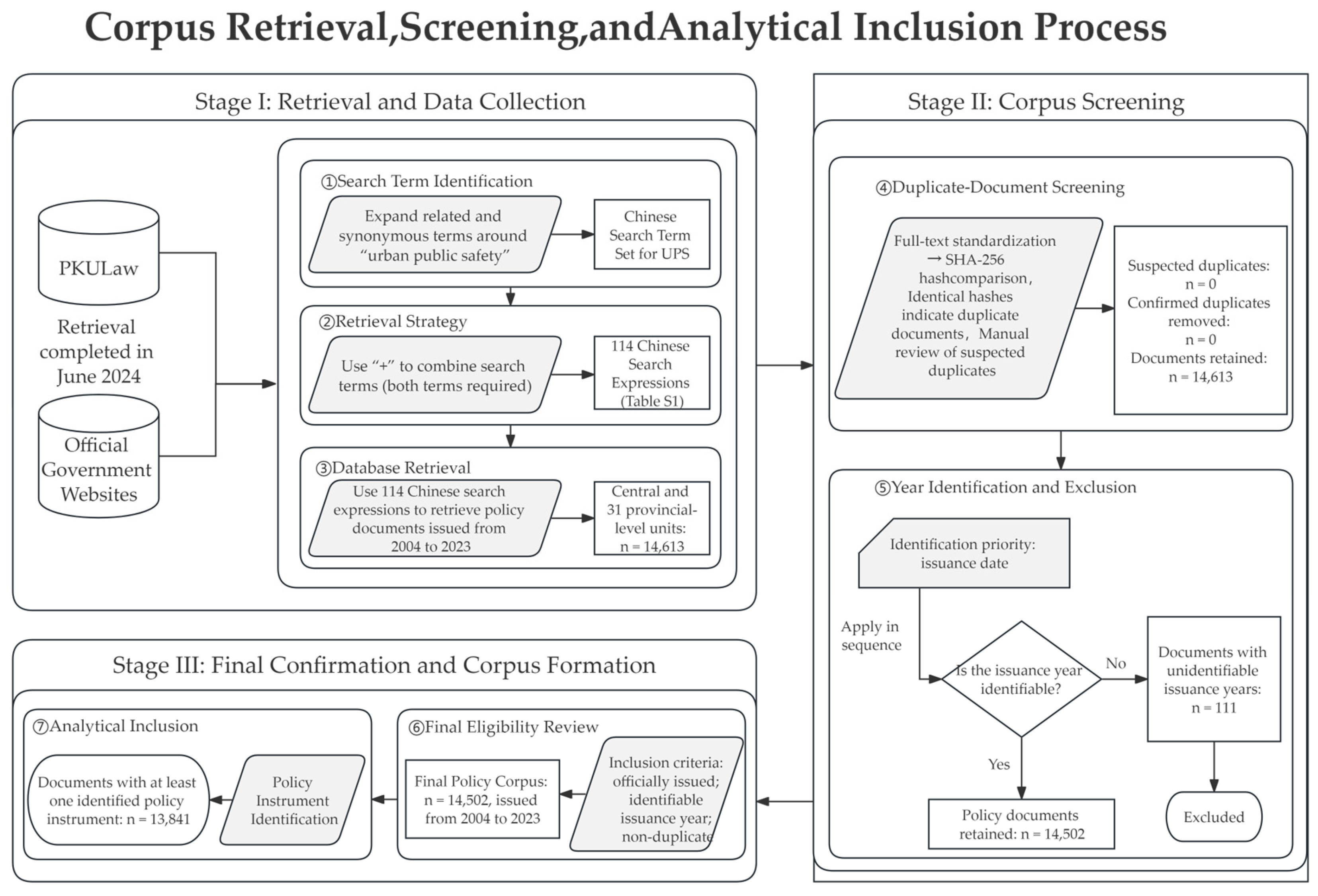
The policy corpus comprises official policy documents related to urban public safety governance collected from PKULaw and official government websites and issued between 2004 and 2023. The retrieval process was completed in June 2024. In PKULaw, central-level retrieval included departmental rules and industry regulations, whereas local-level retrieval included local normative documents, local working documents, and industry regulations. The retrieval strategy used 114 search expressions related to urban public safety governance. The retrieved policy texts underwent a duplicate check, and no repeated documents were identified. After this check was complete and records without identifiable issuance years were excluded, the final corpus comprised 14,502 policy documents issued by the central government and local governments across all 31 provincial-level administrative units. At least one policy instrument was identified in 13,841 of these documents, which formed the textual basis for the subsequent annual co-occurrence analysis. The complete search expressions and annual corpus-exposure statistics are reported in Supplementary Tables S1 and S5, respectively. The corpus retrieval, screening, and final-inclusion procedure are summarized in Figure 2.

Fine-grained policy instruments were identified using a task-specific transformer-based NER model initialized from the pretrained hfl-chinese-roberta-wwm-ext-large checkpoint and fine-tuned using a BIOE sequence-labeling scheme. The training data comprised 3455 sentences with relatively rich policy–instrument content, which were jointly annotated and checked by four public-policy experts, with disagreements resolved through expert voting. Annotation followed predefined semantic and entity-boundary rules, with overlapping or nested spans not retained as multiple independent entities under the flat NER setting. Detailed annotation guidelines are provided in Supplementary Section S2. No formal inter-annotator agreement statistic was calculated for the NER annotation. The model was evaluated using five-fold cross-validation and achieved an F1 score of 89.3%. During inference, text was processed using the model tokenizer, with a sliding-window strategy applied to sequences exceeding the input length. The computing environment for the NER pipeline is reported in Supplementary Table S7.

Following NER extraction, Wenzhong-GPT2-3.5B was used for post-extraction quality control. Perplexity was calculated for each candidate expression, with the median perplexity across all candidate expressions used as the filtering threshold; expressions above the threshold were excluded, and the remaining expressions were retained for subsequent analysis. No external ontology or coding dictionary was used, and no additional synonym merging or ontology-based semantic normalization was applied after NER extraction. Detailed annotation guidelines for policy–instrument identification are provided in Supplementary Section S2.

The policy instruments identified by the NER model were classified according to Schneider and Ingram’s policy–instrument framework [14]. The classification scheme comprised five major categories, namely Authority, Incentive, Capacity, Symbolic and Hortatory, and Learning, which were further operationalized into 38 subcategories. For the five-category classification used in the subsequent network analysis, the classification dataset contained 32,773 labeled records. The dataset was divided into training, validation, and test sets at a ratio of 80:10:10. The classification model, based on hfl-chinese-roberta-wwm-ext-large, was evaluated on a held-out test set of 3278 records. The test set contained no exact text overlap with the training or validation sets. The model achieved a macro precision of 98.59%, macro recall of 98.84%, and macro F1 of 98.71%. The corresponding micro precision, micro recall, and micro F1 were all 99.15%. Category-specific precision, recall, and F1 scores and the confusion matrix are reported in Supplementary Tables S3 and S4. After classification, each identified policy instrument was assigned one of the five major category labels for subsequent network construction and ERGM analysis. The 38-subcategory policy–instrument classification scheme used for category assignment is reported separately in Supplementary Table S2.

3.2. Network Construction

As this study is based on textual analysis, the choice of co-occurrence window affects how policy–instrument relations are identified. Previous text-mining research shows that broader textual windows may introduce more ambiguous or spurious associations, while narrower windows can improve relational precision [21,22,23]. In the present corpus, using paragraphs or entire documents as co-occurrence windows may connect instruments discussed in different provisions or governance tasks. Annual undirected policy–instrument co-occurrence networks are therefore constructed at the sentence level. A tie is defined between two distinct policy instruments when they appear in the same sentence. To characterize both the topology of PIM relations and the distribution of repeated co-occurrences, the descriptive network analysis uses weighted annual networks, as shown in Equation (1). Because the ERGM analysis examines which policy–instrument characteristics and structural properties are associated with the presence of a co-occurrence relation, the weighted annual networks are converted into binary networks for estimation, as shown in Equation (2).

$$w_{ij,t}=\sum _{s\in S_t}{x}_{i,s,t}{x}_{j,s,t}, i\ne j$$

(1)

$$a_{ij,t}=\mathbb{I}(w_{ij,t}>0), i\ne j$$

(2)

where ${\mathrm{S}}_{\mathrm{t}}$ denotes the set of sentences in year $\mathrm{t}$, and ${\mathrm{x}}_{\mathrm{i},\mathrm{s},\mathrm{t}}=1$ if policy instrument $\mathrm{i}$ appears in sentence $\mathrm{s}$ in year $\mathrm{t}$, and 0 otherwise. The weighted edge ${\mathrm{w}}_{\mathrm{i}\mathrm{j},\mathrm{t}}$ counts the number of sentences in which instruments $\mathrm{i}$ and $\mathrm{j}$ co-occur. The binary tie ${\mathrm{a}}_{\mathrm{i}\mathrm{j},\mathrm{t}}$ equals 1 when the two instruments co-occur at least once in year $\mathrm{t}$, and 0 otherwise. Self-loops are excluded by requiring $\mathrm{i}\ne \mathrm{j}$.

3.3. Network Analysis and Indicators

Descriptive network analysis was conducted on the 20 annual policy–instrument co-occurrence networks to characterize the structural features of PIM relations. Four dimensions are examined: network size and density, degree and strength distribution, clustering and assortative mixing, and community structure.

Network size and density are measured by the number of nodes and edges and network density. Degree and strength distributions are characterized by degree centralization, mean node strength, and normalized strength entropy. Clustering and assortative mixing are measured by the global clustering coefficient and weighted-degree assortativity. Community structure is identified using the weighted Louvain algorithm and summarized by the number of communities and weighted modularity. The indicators and formulas are presented in

Table 1. Network Indicators.

Dimension	Indicator	Formula	Meaning in This Study
Network size and density	Number of nodes	${\mathrm{n}}_{\mathrm{t}}=\left|{\mathrm{V}}_{\mathrm{t}}\right|$	Number of policy instruments participating in co-occurrence relations in year t.
	Number of edges	${\mathrm{m}}_{\mathrm{t}}=\left|{\mathrm{E}}_{\mathrm{t}}\right|$	Number of distinct policy–instrument co-occurrence relations in year t.
	Network density	${\mathrm{D}}_{\mathrm{t}}={\displaystyle \frac{2{\mathrm{m}}_{\mathrm{t}}}{{\mathrm{n}}_{\mathrm{t}}({\mathrm{n}}_{\mathrm{t}}-1)}}$	Share of observed co-occurrence ties among all possible policy–instrument pairs.
Degree and strength distribution	Degree centralization	${\mathrm{C}}_{\mathrm{t}}^{\mathrm{D}}={\displaystyle \frac{{\sum }_{\mathrm{i}}({\mathrm{k}}_{\mathrm{m}\mathrm{a}\mathrm{x},\mathrm{t}}-{\mathrm{k}}_{\mathrm{i},\mathrm{t}})}{({\mathrm{n}}_{\mathrm{t}}-1)({\mathrm{n}}_{\mathrm{t}}-2)}}$	Degree to which co-occurrence ties are concentrated around highly connected instruments.
	Mean node strength (weighted degree)	${\stackrel{\mathrm{‾}}{\mathrm{s}}}_{\mathrm{t}}={\displaystyle \frac{1}{{\mathrm{n}}_{\mathrm{t}}}}{\displaystyle \sum _{\mathrm{i}}}{\mathrm{s}}_{\mathrm{i},\mathrm{t}}$	Average cumulative co-occurrence strength of policy instruments.
	Normalized strength entropy	${\mathrm{H}}_{\mathrm{t}}=-{\displaystyle \frac{{\sum }_{\mathrm{i}}{\mathrm{p}}_{\mathrm{i},\mathrm{t}}\mathrm{l}\mathrm{n}({\mathrm{p}}_{\mathrm{i},\mathrm{t}})}{\mathrm{l}\mathrm{n}({\mathrm{n}}_{\mathrm{t}})}}$	Distributional balance of weighted participation across instruments.
Clustering and assortative mixing	Global clustering coefficient	${\mathrm{C}}_{\mathrm{t}}^{\mathrm{G}}={\displaystyle \frac{3{\mathsf{\Delta }}_{\mathrm{t}}}{{\displaystyle {\sum }_{\mathrm{i}=1}^{{\mathrm{n}}_{\mathrm{t}}}}(\genfrac{}{}{0pt}{}{{\mathrm{k}}_{\mathrm{i},\mathrm{t}}}{2})}}$	Proportion of connected triplets that are closed into triangles.
	Weighted-degree assortativity	$r_t^s={\mathrm{c}\mathrm{o}\mathrm{r}\mathrm{r}}_{(i,j)\in E_t}(s_{i,t},s_{j,t})$	Tendency for instruments with similar weighted-degree positions to co-occur.
Community structure	Number of communities	${\mathrm{q}}_{\mathrm{t}}$	Number of policy–instrument co-occurrence communities identified by the weighted Louvain algorithm.
	Weighted modularity	${\mathrm{Q}}_{\mathrm{t}}={\displaystyle \frac{1}{2{\mathrm{W}}_{\mathrm{t}}}}{\sum }_{\mathrm{i},\mathrm{j}}{\mathrm{B}}_{\mathrm{i}\mathrm{j},\mathrm{t}}\mathsf{\delta }({\mathrm{c}}_{\mathrm{i},\mathrm{t}},{\mathrm{c}}_{\mathrm{j},\mathrm{t}})$ ${\mathrm{B}}_{\mathrm{i}\mathrm{j},\mathrm{t}}={\mathrm{w}}_{\mathrm{i}\mathrm{j},\mathrm{t}}-{\displaystyle \frac{{\mathrm{s}}_{\mathrm{i},\mathrm{t}}{\mathrm{s}}_{\mathrm{j},\mathrm{t}}}{2{\mathrm{W}}_{\mathrm{t}}}}$	Extent to which co-occurrence weight is concentrated within communities relative to the weighted null-model expectation.

Note: ${\mathrm{V}}_{\mathrm{t}}$ and ${\mathrm{E}}_{\mathrm{t}}$ denote the node and edge sets in year $\mathrm{t}$; ${\mathrm{k}}_{\mathrm{i},\mathrm{t}}$ is the degree of node $\mathrm{i}$, and ${\mathrm{k}}_{\mathrm{m}\mathrm{a}\mathrm{x},\mathrm{t}}$ is the maximum node degree in year $\mathrm{t}$; ${\mathrm{s}}_{\mathrm{i},\mathrm{t}}={\sum }_{\mathrm{j}}{\mathrm{w}}_{\mathrm{i}\mathrm{j},\mathrm{t}}$ is node strength (weighted degree); ${\mathrm{p}}_{\mathrm{i},\mathrm{t}}={\displaystyle \frac{{\mathrm{s}}_{\mathrm{i},\mathrm{t}}}{{\sum }_{\mathcal{l}\in \mathrm{V}\_\mathrm{t}}{\mathrm{s}}_{\mathcal{l},\mathrm{t}}}}$; ${\mathrm{W}}_{\mathrm{t}}$ is total edge weight; ${\mathrm{c}}_{\mathrm{i},\mathrm{t}}$ is the community membership of node $\mathrm{i}$ in year $\mathrm{t}$; and $\mathsf{\delta }({\mathrm{c}}_{\mathrm{i},\mathrm{t}},{\mathrm{c}}_{\mathrm{j},\mathrm{t}})=1$ if nodes $\mathrm{i}$ and $\mathrm{j}$ belong to the same community in year $\mathrm{t}$, and 0 otherwise. ${\mathsf{\Delta }}_{\mathrm{t}}$ denotes the number of triangles.

.

3.4. ERGM Framework and Variable Measurement

3.4.1. ERGM Model Specification

ERGMs specify the probability distribution of an observed network as a function of selected network statistics [24]. Unlike conventional regression models that assume independence across observations, ERGMs incorporate dependence among network ties as part of the model structure [11,12]. This feature is well suited to policy–instrument co-occurrence networks, as the occurrence of a tie between two instruments can be modeled in relation to both instrument attributes and endogenous network configurations [25]. Because the study compares year-specific associations under changing policy agendas, 20 ERGMs are estimated separately. The general form of an ERGM is shown in Equation (3).

$$P_{\theta }(Y=y\mid X)={\displaystyle \frac{1}{\kappa (\theta ,X)}}\mathrm{e}\mathrm{x}\mathrm{p}\left\{{\theta }^{\mathrm{\top }}g(y,X)\right\}.$$

(3)

where $\mathrm{Y}$ denotes the random network, $\mathrm{y}$ denotes the observed annual policy–instrument co-occurrence network, and $\mathrm{X}$ denotes exogenous instrument attributes. The vector $\mathrm{g}(\mathrm{y},\mathrm{X})$ contains the network statistics specified in the model, $\mathsf{\theta }$ is the corresponding vector of parameters, and $\mathsf{\kappa }(\mathsf{\theta },\mathrm{X})$ is the normalizing constant over all possible networks with the same node set [24].

3.4.2. Variable Selection

The six hypothesized patterns are operationalized through variables and structural statistics representing two dimensions of PIM formation patterns: policy–instrument characteristics and the structural properties of the PIM, with edges included as the network baseline. The corresponding ERGM terms and substantive meanings are summarized in

Table 2. ERGM variables and their explanations.

Variable Type	Variable Statistic	ERGM Term	Substantive Term	Implication	Hypothesis
Baseline network term	Edge	edges	Baseline tie tendency	Baseline propensity to form co-occurrence ties.	—
Policy–instrument characteristics	Usage frequency	nodecov(“tool_freq_log_z”)	Usage frequency	Whether more frequently used instruments are more likely to participate in ties.	H1
	Usage-frequency difference	absdiff(“tool_freq_log_z”)	Usage-frequency difference	Whether instruments differing more in usage frequency are more likely to form ties.	H2
	Policy–instrument category	nodefactor(“tool_major_type”, base = 1)	Category	Whether categories differ in tie participation relative to Authority instruments.	H3
	Category similarity	nodematch(“tool_major_type”)	Category homophily	Whether instruments in the same major category are more likely to form ties.	H4
PIM structural properties	Geometrically weighted degree	gwdegree(0.50, fixed = TRUE)	Degree heterogeneity	Whether co-occurrence ties are unevenly distributed across policy instruments after accounting for attribute-related terms.	H5
	Geometrically weighted edgewise shared partners	gwesp(0.45, fixed = TRUE)	Triadic closure	Whether instruments sharing common co-occurrence partners are more likely to form ties, net of degree heterogeneity.	H6

Note: All ERGM terms are specified for binary undirected annual policy–instrument co-occurrence networks. Usage frequency is measured as the annual number of occurrences of each policy instrument in the policy-text recognition results. Because the raw frequency distribution is strongly right-skewed, the counts are transformed using log1p and then standardized within each year. Usage-frequency difference is calculated as the absolute difference in standardized log-transformed usage frequency between two instruments. Policy–instrument category is coded as a five-category node attribute, with Authority instruments as the reference category. Category similarity is coded as 1 when two instruments belong to the same major category and 0 otherwise.

.

For the geometrically weighted terms, fixed decay parameters were used to control the rate at which the contributions of higher-order degree and shared-partner configurations decline [24,25]. Candidate decay values and parameter combinations were compared through sensitivity analyses, and the final settings were selected based on model performance and estimate stability across the annual networks. These values were then applied consistently to every relevant model specification across all 20 annual networks.

3.4.3. ERGM Specification

To translate the hypotheses into model terms, the ERGM specification is decomposed into baseline tie tendency, policy–instrument attributes, dyadic attribute relations, and endogenous network configurations, as shown in Equation (4).

$${\theta }^{\mathrm{\top }}g(y,X)={\theta }_a{g}_a(y)+{\theta }_b{g}_b(y,X_f)+{\theta }_c{g}_c(y,X_f)+{\displaystyle \sum _{r=1}^4}{\theta }_{d,r}{g}_{d,r}(y,X_c)$$

$$+{\theta }_e{g}_e(y,X_c)+{\theta }_f{g}_f(y)+{\theta }_g{g}_g(y).$$

(4)

In this specification, ${\mathrm{g}}_{\mathrm{a}}(\mathrm{y})$ represents the baseline edge term. ${\mathrm{X}}_{\mathrm{f}}$ denotes annual usage frequency, and ${\mathrm{X}}_{\mathrm{c}}$ denotes policy–instrument category. The usage-frequency statistic ${\mathrm{g}}_{\mathrm{b}}(\mathrm{y},{\mathrm{X}}_{\mathrm{f}})$ corresponds to H1. The statistic for usage-frequency difference, ${\mathrm{g}}_{\mathrm{c}}(\mathrm{y},{\mathrm{X}}_{\mathrm{f}})$ corresponds to H2. The four non-reference category statistics ${\mathrm{g}}_{\mathrm{d},\mathrm{r}}(\mathrm{y},{\mathrm{X}}_{\mathrm{c}})$ ($\mathrm{r}=1,\dots ,4$) correspond to H3, with Authority as the reference category. The category-homophily statistic ${\mathrm{g}}_{\mathrm{e}}(\mathrm{y},{\mathrm{X}}_{\mathrm{c}})$ corresponds to H4. The degree-heterogeneity statistic ${\mathrm{g}}_{\mathrm{f}}(\mathrm{y})$ captures endogenous degree heterogeneity and corresponds to H5. The geometrically weighted edgewise shared-partner statistic ${\mathrm{g}}_{\mathrm{g}}(\mathrm{y})$ captures triadic closure and corresponds to H6. For interpretation, ERGM coefficients are treated as conditional log-odds parameters, with their signs interpreted in relation to the corresponding model statistics while holding the other terms constant. For the geometrically weighted terms, their contributions to the conditional log-odds depend on changes in the corresponding network statistics under the specified fixed decay parameters; accordingly, they are not interpreted as simple marginal effects.

3.5. Estimation Strategy

The annual networks contain an average of 7893 active nodes and 27,981 observed ties. The empirical analysis covers 20 annual policy–instrument co-occurrence networks and seven model specifications for each year, making computational feasibility an important consideration in the estimation design. Markov chain Monte Carlo maximum likelihood estimation (MCMLE) would be substantially more computationally demanding at the scale of the full annual networks. Given these computational constraints, maximum pseudolikelihood estimation (MPLE) was used as the primary estimation strategy because it provides a computationally tractable approach when full-likelihood estimation is too demanding [26]. Uncertainty is summarized using the conventional standard errors returned by the MPLE fit. As MPLE is an approximate estimation approach, its point estimates may differ from full-likelihood estimates, and the conventional MPLE standard errors may not fully capture estimation uncertainty [26]. Accordingly, coefficient estimates and Wald significance tests are interpreted cautiously. Documented software and package versions used for the relevant analyses are reported in Supplementary Table S7.

Model evaluation incorporates two additional diagnostic checks. First, pseudolikelihood-based Akaike information criterion (AIC) and Bayesian information criterion (BIC) values are used as auxiliary information criterion diagnostics [26,27,28]. These values are compared only within the same annual network among models estimated using the same MPLE procedure. Second, goodness-of-fit (GOF) diagnostics are conducted using 500 simulated networks generated from each fitted annual model. These diagnostics assess whether each specification reproduces the model statistics included in that specification [25]. For Models 6 and 7, the extended GOF assessment also examines degree distributions, edgewise shared-partner distributions, geodesic-distance distributions, component structure, global clustering, and isolated nodes; the full extended-GOF summary and representative diagnostic plots are reported in Supplementary Section S8, Table S18 and Figures S1–S4.

Given differences in annual network size and composition, raw ERGM coefficients are not interpreted as directly comparable standardized effect sizes across years; cross-year interpretation focuses on coefficient direction, significance stability, and broad within-term annual patterns. Complete annual coefficient estimates for Models 1–7 are reported in Supplementary Tables S8–S14. To assess sensitivity to annual changes in node composition, Model 6 was also re-estimated on the 77 policy instruments present in all 20 annual networks; the complete strict stable-node sensitivity results are reported in Supplementary Section S7 and Tables S15–S17.

4. Results

4.1. Annual Changes in PIM Structure

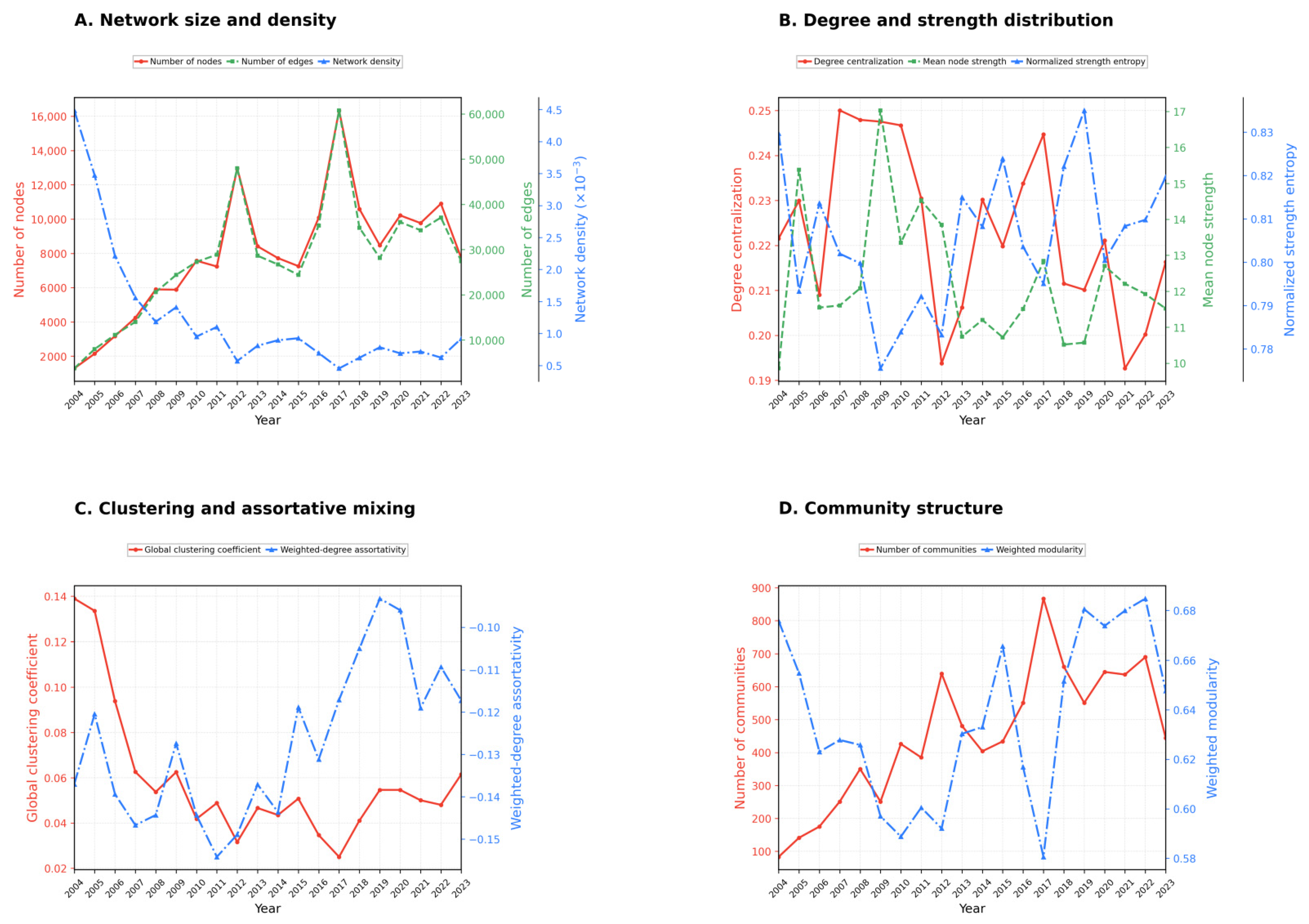
From 2004 to 2023, the annual PIM networks changed across four structural dimensions: network size and density, degree and strength distribution, clustering and assortative mixing, and community structure. Together, these indicators show substantial changes in network scale alongside persistently low density and uneven participation.

The network scale changed substantially from 2004 to 2023, with density generally following the opposite trend. The number of nodes and edges increased overall, from 1286 and 3707 in 2004 to a first local peak in 2012 and then to their maxima in 2017, with 16,344 nodes and 60,799 edges, before falling to 7714 nodes and 27,429 edges in 2023. Density broadly followed the reverse trajectory, falling from its 2004 high of 0.004487 to a first local low in 2012 and then to its minimum of 0.000455 in 2017, before remaining low at 0.000922 in 2023. The share of realized ties among all possible pairs remained very small, even as the PIM incorporated more instruments and co-occurrence ties (Figure 3A).

Because annual corpus exposure varied substantially across the study period, we also examined unique edges relative to policy–instrument mentions. The normalized rate was 1123.7 unique edges per 1000 mentions in 2004, 1488.1 in 2017, and 1529.3 in 2023. Exposure normalization substantially attenuated the apparent expansion in raw network scale, and the 2017 peak in raw edges was no longer a peak after adjustment. At the same time, the normalized rates in later years generally remained above the 2004 level, indicating that variation in corpus exposure alone did not fully account for the observed changes in network scale (Supplementary Table S5).

The mean node strength and normalized strength entropy generally moved in opposite directions, indicating that stronger weighted participation was typically accompanied by a more uneven distribution of co-occurrence strength across instruments. The connection concentration was relatively stronger in the earlier years. Degree centralization reached its maximum of 0.250 in 2007, and the mean node strength subsequently peaked at 17.031 in 2009, when normalized strength entropy fell to its minimum of 0.776. Thereafter, degree centralization declined to its minimum of 0.193 in 2021. By 2023, mean node strength had fallen to 11.518, while the normalized strength entropy was 0.820. These changes indicate a relatively more distributed pattern of weighted participation after the 2009 concentration peak, although unevenness remained (Figure 3B).

The global clustering coefficient remained below 0.14 throughout the observation period, indicating that closed triplets accounted for only a small share of connected triplets. Its trajectory broadly tracked that of network density, with both indicators declining overall as the PIM expanded and recovering somewhat after 2017. The global clustering coefficient was highest at 0.139 in 2004, declined to 0.032 in 2012, and reached its minimum of 0.025 in 2017 before recovering to 0.062 in 2023. The weighted-degree assortativity was negative in every year and reached its peak negative value of −0.154 in 2011. It generally moved closer to zero thereafter, reaching −0.093 in 2019 before ending at −0.117 in 2023. This persistent disassortative pattern indicates that instruments with a higher weighted degree tended to connect with those with a lower weighted degree (Figure 3C).

The number of communities closely tracked the trajectory of the network size. The community count increased from 83 in 2004 to a first local peak of 640 in 2012 and then to its highest value of 867 in 2017 before declining to 444 in 2023. This trajectory shows that the expansion of the PIM generated more distinguishable policy–instrument co-occurrence communities. Despite the expansion and contraction in the number of communities, the weighted modularity remained substantial, ranging from 0.581 to 0.685 and reaching its maximum in 2022. These values indicate that co-occurrence weight remained concentrated within communities relative to the modularity null model, indicating persistent modular differentiation across the annual networks (Figure 3D). Complete annual descriptive network statistics are reported in Supplementary Table S6.

4.2. ERGM-Based Association Analysis

The ERGM analysis proceeds through seven nested specifications: Models 1–5 sequentially introduce the baseline and policy–instrument characteristic terms, Model 6 adds degree heterogeneity as the primary structural specification, and Model 7 adds triadic closure as a diagnostic extension (

Table 3. ERGMs.

Model	Variable	Added Term	Purpose
M1	Baseline	edges	Sets the baseline tendency for policy instruments to form co-occurrence ties.
M2	Usage Frequency	M1 + nodecov(“tool_freq_log_z”)	Tests whether instruments with higher usage frequency are more likely to participate in co-occurrence ties.
M3	Category	M2 + nodefactor (“tool_major_type”, base = 1)	Tests whether policy–instrument categories differ in co-occurrence participation relative to Authority instruments.
M4	Category Homophily	M3 + nodematch(“tool_major_type”)	Tests whether instruments in the same major category are more likely to co-occur.
M5	Usage-Frequency Difference	M4 + absdiff(“tool_freq_log_z”)	Tests whether instruments with larger usage-frequency differences are more likely to form co-occurrence ties.
M6	Degree Heterogeneity	M5 + gwdegree (0.50, fixed = TRUE)	Tests whether co-occurrence ties remain concentrated around highly connected instruments after policy–instrument characteristics are included.
M7	Triadic Closure	M6 + gwesp (0.45, fixed = TRUE)	Tests whether instruments sharing common co-occurrence partners are more likely to form co-occurrence ties.

Note: Models are estimated separately for each annual binary network from 2004 to 2023. Authority instruments are the reference category for the category term in Models 3–7.

).

Table 4. Mean Coefficients and Stability.

Term	M1	M2	M3	M4	M5	M6 Main Model	M7
Edges	−6.883 (20/20; −)	−7.672 (20/20; −)	−7.681 (20/20; −)	−8.389 (20/20; −)	−8.401 (20/20; −)	−8.265 (20/20; −)	−11.552 (20/20; −)
Usage Frequency	—	0.574 (20/20; +)	0.574 (20/20; +)	0.576 (20/20; +)	0.570 (20/20; +)	0.552 (20/20; +)	0.230 (20/20; +)
Category: Capacity instruments	—	—	0.081 (17/20; +17/−3)	0.375 (20/20; +)	0.375 (20/20; +)	0.376 (20/20; +)	0.292 (20/20; +)
Category; Incentive instruments	—	—	−0.095 (15/20; +6/−14)	0.408 (20/20; +)	0.410 (20/20; +)	0.416 (20/20; +)	0.489 (20/20; +)
Category; Learning instruments	—	—	−0.101 (17/20; +1/−19)	0.348 (20/20; +)	0.349 (20/20; +)	0.351 (20/20; +)	0.261 (19/20; +19/−1)
Category; Symbolic and Hortatory instruments	—	—	−0.051 (10/20; +4/−16)	0.435 (20/20; +)	0.437 (20/20; +)	0.443 (20/20; +)	0.255 (18/20; +18/−2)
Category Homophily	—	—	—	0.842 (20/20; +)	0.842 (20/20; +)	0.842 (20/20; +)	0.648 (20/20; +)
Usage-Frequency Difference	—	—	—	—	0.010 (11/20; +14/−6)	0.021 (17/20; +18/−2)	0.048 (20/20; +)
Degree Heterogeneity	—	—	—	—	—	−0.756 (20/20; −)	−5.550 (20/20; −)
Triadic closure	—	—	—	—	—	—	4.154 (20/20; +)

Note: Entries are mean coefficients across the 20 annual models. Parentheses report the number of annual estimates significant at p < 0.05 and coefficient direction; when coefficient directions vary across years, the numbers of positive and negative coefficients are reported. Mean coefficients are descriptive within-term summaries across annual models; they are not standardized effect sizes and should not be compared directly across different ERGM terms. Authority instruments are the reference category for the four categories of coefficients.

summarizes mean coefficients, significance stability, and directional consistency across the 20 annual policy–instrument co-occurrence networks. The results support retaining Model 6 as the main model. The edge term is negative in every model and every year. Meanwhile, the usage frequency coefficient remains positive and significant once introduced. Category coefficients become more stable after the inclusion of category homophily, which remains positive and significant from Model 4 onward. The usage-frequency difference coefficient is small and less consistently significant in Model 5 but becomes more consistently positive and significant after degree heterogeneity is included in Model 6; in this model, it is negative and significant in all annual networks. Model 7 adds triadic closure, which is positive and significant at the coefficient level, while its diagnostic performance is assessed separately in the GOF and closure-check sections.

Table 5. Pseudolikelihood-Based AIC and BIC Comparison.

Model	Available Years	Pseudo-AIC Lower than Previous	Pseudo-BIC Lower than Previous
M1	20	—	—
M2	20	20/20	20/20
M3	20	19/20	18/20
M4	20	20/20	20/20
M5	20	13/20	8/20
M6	20	20/20	19/20
M7	20	20/20	20/20

Note: The last two columns report the number of annual networks in which each model has a lower pseudo-AIC or pseudo-BIC than the immediately preceding model.

provides an auxiliary within-year comparison based on pseudo-AIC and pseudo-BIC, which are considered together with GOF diagnostics. Relative to Model 5, Model 6 has a lower pseudo-AIC in all 20 annual networks and a lower pseudo-BIC in 19; although Model 7 further reduces both criteria in all 20 years, its substantially weaker fitted-statistic reproduction does not support replacing Model 6 as the primary specification.

4.3. Network Sparsity and Low Tie Propensity

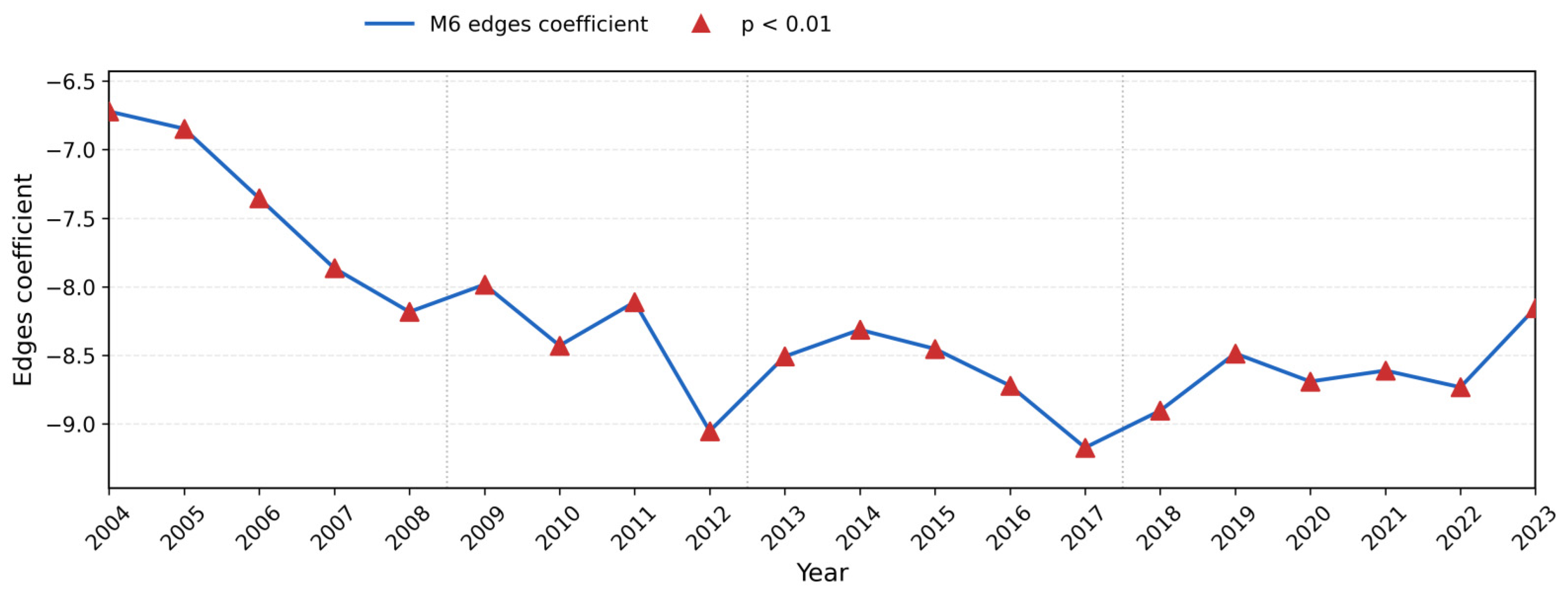
As shown in Table 4, the edge coefficient is negative and statistically significant in all 20 annual networks and every ERGM model, indicating a low baseline propensity for policy–instrument ties. In the main model (Figure 4), the coefficient reaches its maximum in 2004, when the network is smallest, and local minima of −9.052 in 2012 and −9.172 in 2017, when the network reaches its largest observed scale; after 2018, the coefficient fluctuates within a narrower range. During the expansion period, the coefficient remained clearly negative, indicating that greater network scale did not translate into a higher baseline propensity for tie occurrence.

4.4. Policy–Instrument Characteristics

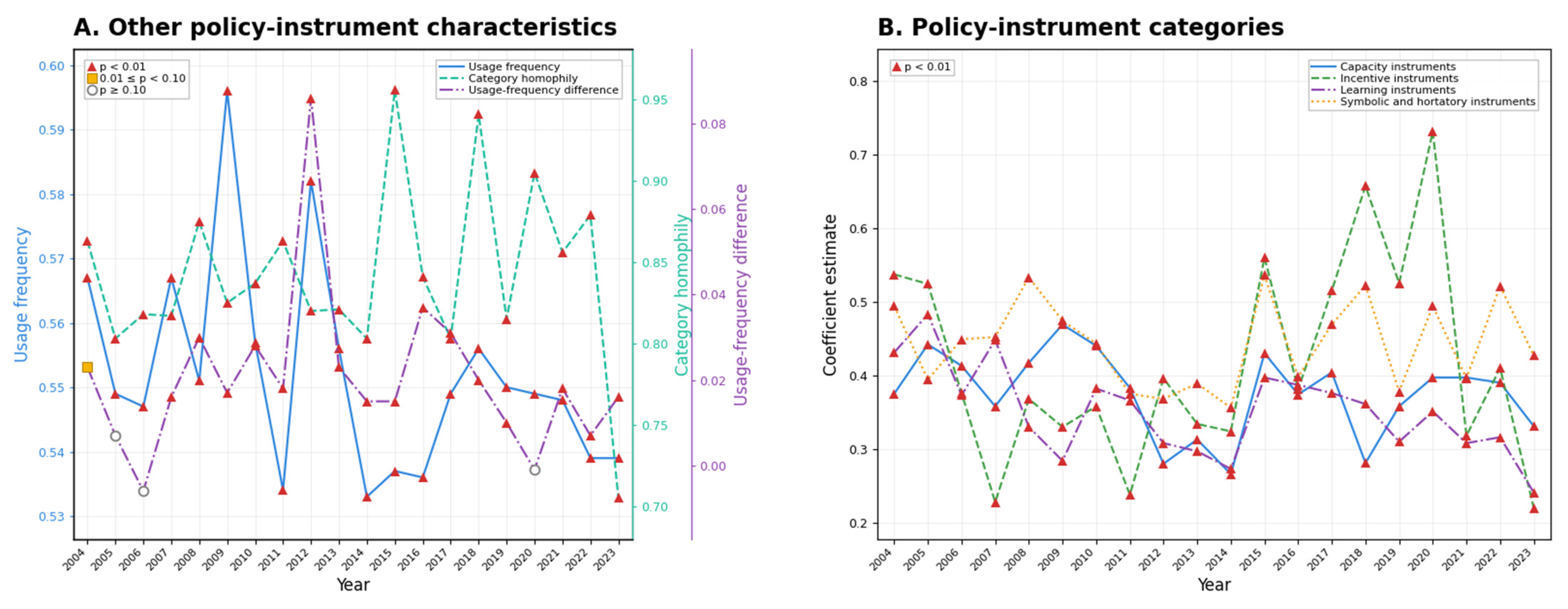
This section examines four policy–instrument characteristics in the main model: usage frequency, usage-frequency difference, category, and category homophily. Figure 5 presents their annual coefficient trends.

The usage frequency coefficient is positive and statistically significant in all 20 annual networks across Models 2–6, with a mean coefficient of 0.552 in Model 6. It reaches a first high of 0.596 in 2009 and another high of 0.582 in 2012 before declining and stabilizing after 2014 (Figure 5A). These results show a stable conditional association between higher annual usage frequency and participation in co-occurrence ties, supporting H1.

All non-reference policy–instrument categories exhibit positive and statistically significant participation tendencies relative to Authority instruments after category homophily and endogenous network structure are accounted for. In the main model, Capacity, Incentive, Learning, and Symbolic and Hortatory instruments have mean coefficients of 0.376, 0.416, 0.351, and 0.443, respectively. The Capacity coefficient is relatively higher in the earlier years, reaching 0.469 in 2009; it declines during 2012–2014 before recovering. The Learning coefficient reaches its maximum of 0.483 in 2005 and is lower in the middle years. The Incentive coefficient is relatively lower during 2006–2014 but increases after 2015, reaching its maximum of 0.731 in 2020. Symbolic and Hortatory instruments have the highest mean coefficient among the four non-reference category contrasts but show pronounced year-to-year fluctuations (Figure 5B). These results offer conditional support for H3.

The homophily coefficient category remains consistently positive and statistically significant in all 20 annual networks across Models 4 to 6, with a mean coefficient of 0.842 in the main model. The coefficient is relatively higher in several later years, reaching 0.956 in 2015 and 0.941 in 2018, while most annual values remain around 0.80 (Figure 5A). Policy instruments within the same category are more likely to form co-occurrence ties, consistent with homophily theory and policy–instrument classification theory. Instruments within the same category share closer governing logics, behavioral assumptions, and functional orientations, increasing their likelihood of entering the same co-occurrence context. Consistent with this tendency, authority-oriented instruments may cluster around regulation, supervision, inspection, enforcement, and responsibility assignment. These results support H4.

The usage-frequency difference coefficient becomes more consistently positive and significant after degree heterogeneity is included in the main model. Its mean coefficient is 0.021; estimates are positive in 18 of the 20 annual networks and statistically significant in 17, while the two negative estimates, in 2006 and 2020, are not statistically significant. The coefficient reaches its maximum of 0.086 in 2012; outside that year, annual estimates remain comparatively small (Figure 5A). These results indicate that instruments with larger usage-frequency differences are more likely to form co-occurrence ties after degree heterogeneity has been accounted for. This pattern may reflect the pairing of higher-frequency instruments that provide broad governance frames with lower-frequency instruments that specify more task-oriented actions within the same PIM. These results offer conditional support for H2.

4.5. PIM Structural Properties

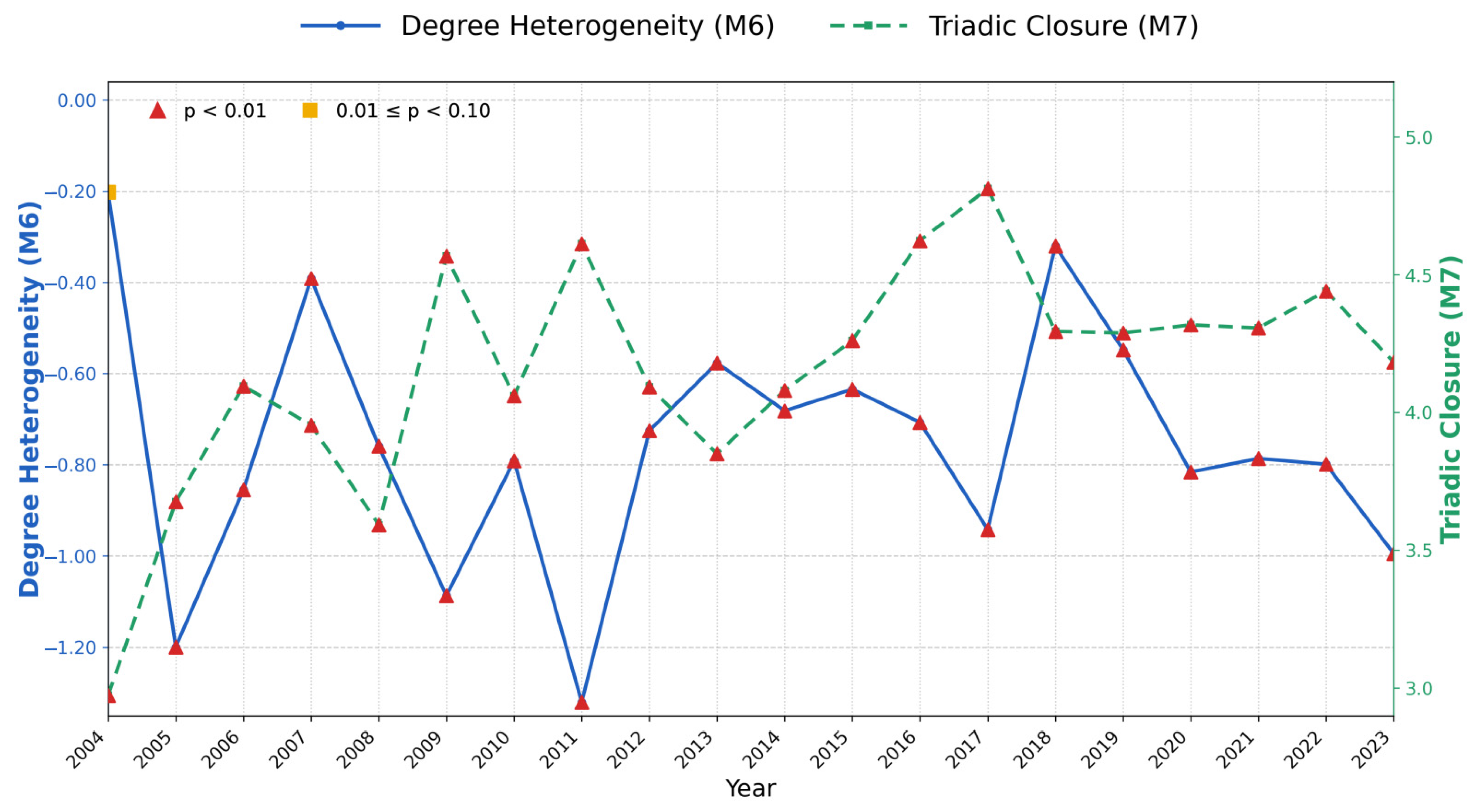
This section examines two PIM structural properties: degree heterogeneity in the main model and triadic closure in Model 7. Figure 6 illustrates their annual coefficient trends.

The degree heterogeneity coefficient is negative and statistically significant in all 20 annual networks in the main model, with a mean coefficient of −0.756. The coefficient is −0.201 in 2004 and reaches its minimum of −1.320 in 2011. After 2012, annual coefficients generally fluctuate within a narrower negative range, apart from a relatively higher value in 2018 (Figure 6). The consistently negative degree-heterogeneity coefficients provide conditional evidence of uneven tie concentration after the other model terms are accounted for. A smaller set of instruments, including organization and supervision, repeatedly co-occurred across risks, sectors, and governance tasks and occupied highly connected positions in the policy–instrument co-occurrence network throughout the observation period. Taken together, these results support H5.

The triadic closure coefficient is positive and statistically significant in all 20 annual networks in the triadic-closure model, with a mean coefficient of 4.154. These coefficient results indicate that instruments sharing common co-occurrence partners are more likely to form additional co-occurrence ties. However, the triadic-closure model reproduces its fitted model statistics substantially less well than the main model. The results provide conditional support for H6 at the coefficient level, while the deterioration in fitted-statistic GOF indicates that triadic closure should be retained as a diagnostic extension rather than used as a replacement for the main model.

4.6. Goodness-of-Fit Diagnostics

Table 6. GOF Diagnostics.

Model	Years	GOF Statistics	p < 0.05	p < 0.10	Mean p-Value
M1	20	20	0/20 (0.0%)	0/20 (0.0%)	0.716
M2	20	40	1/40 (2.5%)	2/40 (5.0%)	0.520
M3	20	120	5/120 (4.2%)	11/120 (9.2%)	0.519
M4	20	140	3/140 (2.1%)	10/140 (7.1%)	0.548
M5	20	160	5/160 (3.1%)	9/160 (5.6%)	0.533
M6	20	180	9/180 (5.0%)	17/180 (9.4%)	0.509
M7	20	200	141/200 (70.5%)	152/200 (76.0%)	0.117

Note: The columns p < 0.05 and p < 0.10 report the number and percentage of GOF statistics with low Monte Carlo p-values. Each annual GOF assessment is based on 500 simulated networks.

summarizes the goodness-of-fit diagnostics for the statistics included in the fitted ERGMs. For Model 6, 9 of 180 fitted statistics have p-values below 0.05; 17 fall below 0.10; and the mean p-value is 0.509. Additionally, 171 of the 180 statistics fall within the pointwise 95% simulation intervals. Model 7 shows substantially weaker fitted-statistic reproduction: 141 of 200 statistics have p-values below 0.05, 152 fall below 0.10, the mean p-value is 0.117, and only 59 of the 200 statistics fall within the pointwise 95% simulation intervals. Therefore, Model 6 reproduces the fitted statistics well, although its reproduction of out-of-model network properties varies across structural dimensions. Within the theoretically specified candidate model sequence, Model 6 provides the most defensible balance between diagnostic performance and substantive interpretability and is retained as the primary specification for association-oriented interpretation. Extended GOF summary results across all 20 annual networks are reported in Supplementary Table S18, with representative diagnostic plots for 2017 provided in Figures S1–S4.

4.7. Robustness Checks

The additional closure checks clarify why triadic closure is retained as a diagnostic extension rather than as the main structural specification. When policy–instrument characteristics and triadic closure are included without degree heterogeneity, the triadic closure coefficient remains consistently positive and statistically significant in all 20 annual networks, with a mean coefficient of 2.890. However, this model still shows weaker diagnostic performance than the main model: 52 of 180 statistics have p-values below 0.05, 76 fall below 0.10, and the mean p-value is 0.255. The structural closure check offers a sharper diagnosis. When only the edge term, degree heterogeneity, and triadic closure are included, all 60 goodness-of-fit statistics have p-values below 0.05, with a mean p-value of 0.000. This result pinpoints the joint structural specification of degree heterogeneity and triadic closure as the main source of diagnostic deterioration. These checks support retaining the main model for substantive interpretation and interpreting H6 as conditionally supported at the coefficient level. The corresponding structural-specification diagnostics are summarized in

Table 7. Structural Specification Diagnostics.

Model	Check	Coefficient Evidence	GOF Diagnostics	Interpretation
M6	Main model	Triadic closure not included.	p < 0.05: 9/180; p < 0.10: 17/180; mean p-value: 0.509	Retained as the main model.
M7	Triadic-closure model	Triadic closure mean coefficient: 4.154; positive and significant in 20/20 annual networks.	p < 0.05: 141/200; p < 0.10: 152/200; mean p-value: 0.117	Triadic closure is detectable, but fitted-statistic reproduction is weak.
M8	Attribute + triadic closure model	Triadic closure mean coefficient: 2.890; positive and significant in 20/20 annual networks.	p < 0.05: 52/180; p < 0.10: 76/180; mean p-value: 0.255	Closure evidence remains, but diagnostic support is weaker than the main model.
M9	Structural closure check	Triadic closure mean coefficient: 4.685; positive and significant in 20/20 annual networks. Degree heterogeneity mean coefficient: −8.262.	p < 0.05: 60/60; p < 0.10: 60/60; mean p-value: 0.000	The diagnostic problem is strongest when degree heterogeneity and triadic closure are combined.

Note: Low p-values indicate local diagnostic warnings. The GOF diagnostics evaluate the statistics included in each fitted model. Each annual GOF assessment is based on 500 simulated networks.

.

To assess whether the main results depend on one-off co-occurrences, the sensitivity analysis retained only policy–instrument pairs that co-occurred in at least two sentences within the same year; all other model settings were kept identical to Model 6. The alternative threshold reduced the mean number of active nodes from 7893 to 2259 and the mean number of edges from 27,981 to 6367; annual node and edge retention ranged from 26.2–32.8% and 19.9–26.1%, respectively.

Compared with Model 6, usage frequency, all four non-reference category coefficients, and category homophily retained the same positive direction and statistical significance in all 20 annual networks under the alternative threshold. The usage-frequency difference remained significant in 17 years and was positive in all 20 years under the alternative threshold, compared with 18 positive years in Model 6.

Degree heterogeneity showed a sign reversal under the alternative threshold, but remained statistically significant in 18 of the 20 annual networks, indicating that degree structure remained associated with PIM formation despite the change in direction. Its annual coefficient trajectory also remained closely aligned with that of Model 6 (Spearman’s ρ = 0.866; Pearson’s r = 0.805), showing that the year-to-year pattern of this structural association was largely preserved. The sign reversal can also be understood in light of the change in network composition under the stricter threshold. Removing one-off co-occurrence ties also removes many low-degree nodes, changing the degree distribution and weakening the concentration of ties around a small number of highly connected instruments, which helps to explain the positive coefficients observed in most years. The corresponding sensitivity results are summarized in

Table 8. Sensitivity Analysis Using an Alternative Co-occurrence Threshold.

ERGM Term	Model 6 Mean	Alternative-threshold Mean	Model 6 Direction	Alternative Direction	Model 6 Significant Years	Alternative Significant Years
Usage frequency	0.552	0.704	+20/−0	+20/−0	20/20	20/20
Category: Capacity	0.376	0.477	+20/−0	+20/−0	20/20	20/20
Category: Incentive	0.416	0.554	+20/−0	+20/−0	20/20	20/20
Category: Learning	0.351	0.469	+20/−0	+20/−0	20/20	20/20
Category: Symbolic and Hortatory	0.443	0.529	+20/−0	+20/−0	20/20	20/20
Category homophily	0.842	1.046	+20/−0	+20/−0	20/20	20/20
Usage-frequency difference	0.021	0.048	+18/−2	+20/−0	17/20	17/20
Degree heterogeneity	−0.756	0.294	+0/−20	+16/−4	20/20	18/20

Note: Mean coefficients are descriptive summaries across the 20 annual models. Direction reports the number of positive and negative annual coefficients. Significant years report the number of annual estimates with p < 0.05.

.

5. Discussions and Conclusions

This study examined how PIMs are formed in China’s UPS policy from 2004 to 2023. Methodologically, this study develops a fine-grained measurement strategy that combines NER-based policy–instrument identification and classification with network-based relational analysis. This strategy offers greater granularity than category-only or frequency-based approaches. Using this strategy, this study further unpacks PIM formation by examining six patterns across two dimensions: policy–instrument characteristics (usage frequency, usage-frequency difference, instrument category, and category homophily) and structural properties of the PIM (degree heterogeneity and triadic closure). This approach provides a more detailed understanding of PIM formation and internal organization in China and could also be applied to PIM research in other countries facing complex and cross-sectoral governance challenges.

A central finding is that annual PIM networks expanded substantially, but the observed combinations still accounted for only a small share of all possible policy–instrument pairings. Descriptive network analysis shows that when annual networks expanded, the numbers of policy instruments, ties, and communities increased, whereas network density continued to decline and remained low. The ERGM results further support this pattern: the edge coefficients remained negative across all 20 years, indicating a consistently low baseline propensity for policy instruments to form co-occurrence ties after accounting for the included policy–instrument characteristics and network configurations. These results show that increasing the number of policy instruments does not automatically produce more extensively connected PIMs. For policy design, adding more instruments alone may therefore be insufficient. When new risks and governance demands require additional instruments, attention should also be paid to how they fit with existing instruments and where coordination is needed. This may help policymakers develop more coherent PIMs as the range of policy responses expands.

We also found that policy instruments participated unevenly in PIM formation. In the descriptive network analysis, weighted-degree assortativity remained negative, indicating that highly connected instruments consistently formed combinations with low-connectivity instruments. The ERGM results provided further confirmation of this uneven pattern. Degree heterogeneity remained negative across all 20 years in the main model. The results show that, after accounting for the other model terms, connections tended to concentrate around instruments that were already highly connected. These findings indicate that highly connected instruments may serve as stable connection points across different governance tasks. Such a configuration may help link established policy responses with more targeted instruments when new risks and governance demands emerge, which may support more timely and flexible policy adjustment. For policy design, this may provide a practical way to balance continuity and adjustment. It may also offer useful lessons for other countries, particularly developing countries facing rapidly changing and cross-sectoral public safety challenges.

A third finding is that frequently used policy instruments and instruments within the same category consistently showed a higher likelihood of being combined. The ERGM results show that both usage frequency and category homophily remained positive and statistically significant across all 20 years and under the alternative co-occurrence threshold. The repeated use of these instruments across different policy contexts may help maintain stability in policy design as risks and governance demands change. Category homophily indicates that instruments with similar governing logics and functional orientations are more likely to be organized together. This suggests a degree of specialization and focus in China’s UPS policy design. Such targeted combinations may also help improve the efficiency of policy implementation. Taken together, these features may provide a stable and focused basis for addressing complex public safety problems.

Finally, the annual variation in PIM formation can be understood in relation to major shifts in China’s UPS policy agenda. Following the severe acute respiratory syndrome outbreak in 2003, China’s crisis-management system entered a more institutionalized phase and gradually developed toward a more comprehensive emergency-management framework [29]. After the 2008 Wenchuan earthquake, changes in the PIM became more pronounced. In 2009, the mean node strength reached its peak, and the usage-frequency effect rose to one of its highest levels, which was indicative of increased participation from frequently used instruments. Policy learning and subsequent reforms during this period placed greater emphasis on risk prevention, emergency planning and preparedness, local responsibility, and coordination across jurisdictions [30]. By 2012, network size and the number of communities reached their first local peaks, while the usage-frequency difference effect reached its maximum. These changes occurred as increasingly complex urban risks highlighted integrated risk prevention and broader urban public safety governance [31]. The PIM continued to expand from 2013 to 2017 and reached its largest observed scale in 2017, alongside continued reforms in areas such as safety production and emergency-system planning. From 2016 onward, urban safety received greater policy attention, with the national urban-safety agenda becoming more explicit in 2018 and the establishment of the Ministry of Emergency Management further integrating previously dispersed disaster- and safety-related functions [29,32]. After 2018, the network scale declined from its 2017 peak, while category-based combinations remained prominent and weighted participation became more evenly distributed. These changes indicate a shift from continued expansion toward adjustment in PIM formation. Overall, the correspondence between these empirical changes and major shifts in China’s UPS governance may indicate that policy–instrument use was adjusted in a timely manner as public safety risks and governance demands changed.

Future research can extend this analysis in three directions. First, policy-text processing and validation can be further improved. Independent double coding could be used for NER annotation, with inter-annotator agreement formally reported. Co-occurrence windows defined by sentences, paragraphs, and entire documents could be compared to examine whether different textual windows affect the identified PIM patterns. Second, network modeling and validation can be further improved. Given that MCMLE is computationally demanding for large networks and MPLE may be less accurate, more suitable estimation methods could be explored to better balance accuracy and computational feasibility. Complete token counts could also be retained for additional exposure-normalized analyses. Weighted network models could be compared with binary networks to assess the robustness of the identified PIM patterns. Dynamic network models could also be used to examine temporal dependence in PIM formation. Third, implementation records, administrative process documents, departmental collaboration data, interviews, and case evidence could be incorporated to examine whether PIMs identified in policy texts are also reflected in actual governance processes.