LLM-Driven Signal Control Method for Signalized Intersections with Mixed Traffic Flow

Highlights

Please indicate how your work links to systems science via your contributions to systems practice, theory, and/or methodology.

• Develops a three-layer perception–decision–execution framework that couples LLM-driven signal control with CAV speed guidance in mixed traffic.
• Treats intersection control as a connected vehicle–infrastructure system, integrating real-time traffic states and non-recurrent operational constraints within a unified control process.

What are the main findings and/or the implications of the main findings?

• Controlled SUMO simulations show that coordinating signal decisions with CAV speed guidance improves delay performance, with the benefit generally becoming more evident as connected-vehicle information increases.
• The framework responds to emergency-vehicle priority and road-construction constraints without scenario-specific LLM training and maintains workable performance under varying traffic demand and perception noise.

Abstract

With the development of artificial intelligence and automated driving technologies, traffic signal control is evolving toward greater flexibility and faster response. From the perspective of the Transportation Cyber-Physical System (T-CPS), this paper focuses on mixed traffic scenarios involving connected and automated vehicles (CAVs) and human-driven vehicles (HVs). It proposes integrating a Large Language Model (LLM) into signal control: roadside devices perceive traffic states, prompt engineering is constructed, and the LLM is driven to reason and generate control signals. On this basis, a CAV speed guidance algorithm is proposed. Controlled SUMO simulations of a single isolated intersection under ideal V2X communication assumptions show that the proposed method improves delay performance under the tested mixed-traffic conditions. As the CAV penetration rate increases, traffic performance is further improved. Additional experiments under emergency-vehicle priority, road-construction constraints, different traffic-demand levels, perception noise, and different decision intervals and guidance ranges provide simulation-based evidence of training-free scenario adaptability and robustness within the examined scope. Although inference latency and remote-API delays constrain the timely availability of fresh LLM actions, the hard-deadline policy and deterministic fallback mechanism maintain continuous signal execution and favorable traffic performance in the controlled SUMO simulations.

1. Introduction

As the number of vehicles increases, urban traffic congestion has become more serious, particularly at intersections with limited capacity. For isolated intersections under saturated traffic conditions, traditional signal control methods have evolved from fixed-time designs such as Webster’s formula to actuated and adaptive systems like SCOOT [1] and SCATS [2]. Although these methods rely on model-based optimization and can improve performance under recurring patterns, they still struggle to maintain decision accuracy in highly complex and fluctuating traffic scenarios. For instance, traditional adaptive control uses model-based algorithms for dynamic optimization but still faces the bottleneck of insufficient decision-making accuracy in complex traffic scenarios [3,4,5]. To solve this problem, researchers have proposed several improvements: Ren proposed an adaptive signal control method to address intersection blockage caused by queue spillovers. By triggering early green termination (ECG) or return of unused green (RUG) through speed thresholds, this approach can prevent congestion but fails to systematically optimize global metrics such as delay, throughput, and fairness [6]. In contrast, Xie developed a distributed, comprehensive adaptive control framework based on shockwave theory, which not only prevents queue spillovers at their source but also achieves multi-objective global optimization encompassing delay, throughput, fairness, and network coordination [7].

In contrast, reinforcement-learning-based control methods emphasize learning from data and offer stronger flexibility in unknown scenarios [8,9,10]. Early reinforcement learning mainly used tabular methods such as Q-learning to store the Q-values of state-action pairs for determining signal phases and durations [11,12,13]. In complex road network scenarios, because the state space contains multidimensional information such as vehicle positions, speeds, and signal phases at multiple intersections, tabular methods face significant limitations [14]. For this reason, deep reinforcement learning methods, such as the Deep Q-Network (DQN), have been introduced into traffic signal control. However, when DQN evaluates the expected returns of different actions, it relies on only one Q function, which may overestimate the benefits brought by some actions beyond their actual level [15]. Therefore, scholars have adopted double Q-network models that separate selecting the optimal action from evaluating the value of that action. For example, Wang [16] constructed a double deep Q-network incorporating a convolutional block attention module, which can automatically focus on the distribution and dynamics of vehicles near intersections to optimize traffic signal control. In addition, Actor-Critic methods have attracted scholarly attention. Chu [3] optimized traffic signal control strategies through the actor module and evaluated policy values through the critic module to reduce learning variance, thereby achieving adaptive and efficient signal control in complex traffic environments. Proximal Policy Optimization (PPO) is also a widely used policy gradient algorithm that is commonly implemented using an Actor–Critic architecture and has been applied to adaptive traffic signal control [17,18].

Reinforcement learning methods show advantages in control performance and data processing capability, but their inherent limitations still deserve attention. On one hand, insufficient model generalization constrains their performance in cross-scenario applications; on the other hand, excessive reliance on pretraining data may reduce their adaptability to dynamic traffic demand [19]. To cope with the complex fluctuations of future urban traffic demand, intelligent signal controllers need stronger dynamic perception capability and scenario adaptability. Recently, as an important advance in artificial intelligence, LLMs have been widely applied in many parts of intelligent transportation systems, such as traffic accident prediction [20], bus holding control [21], mixed-vehicle parking rules [22], cross-scenario autonomous decision-making for automated driving [23], and UAV monitoring systems [24]. In traffic signal control, Masri [25] proposed an LLM signal control method that considers conflict identification; Wang et al. [26] used the more comprehensive human-like judgment logic of LLMs to make RL-based signal controllers less dependent on reward functions; Movahedi [27] introduced the ability of LLM reasoning to generate signal control strategies and improved traditional Actor-Critic signal control methods; and Yao et al. [19] constructed a vision-integrated LLM signal control model. Overall, LLM methods can manage complex environmental data and task instructions, extract basic features from multimodal observations, and analyze the causes of failed task execution. In essence, this inherits and develops the dynamic optimization logic of learning-based methods.

Beyond infrastructure-side signal control, LLMs and vision-language models have been more extensively investigated for autonomous-driving decision-making and vehicle control. DiLu introduced LLM-based reasoning, memory, and reflection for knowledge-driven driving decisions [28]; LMDrive and DriveGPT4 incorporated multimodal observations and language instructions into closed-loop end-to-end driving [29,30]; Driving with LLMs generated explainable driving actions from object-level representations [31]; and DriveLM and DriveVLM connected scene perception with prediction, behavioral planning, and vehicle motion generation [32,33]. Moraga et al. further explored LLM-generated network-level speed recommendations using traffic information collected through UAV and IoT systems [24]. Although these approaches can reason about interactions among multiple road users, their decision outputs are predominantly ego-vehicle-centric, focusing on behavioral planning, trajectory generation, or direct control of an individual automated vehicle. Connectivity-enabled coordination between an infrastructure signal controller and multiple CAVs and HVs has generally not been explicitly considered.

Before the connected environment is fully deployed, CAVs and HVs will coexist on urban roads for a considerable period, making mixed-traffic control at signalized intersections a practically important research topic [34,35,36]. Recent studies have shown that coordinated signal control and CAV-level control can improve intersection operations in mixed traffic. Maadi et al. combined reinforcement-learning-based signal planning with vehicle speed guidance in a connected and automated vehicle environment [37]. Related low-penetration adaptive signal control using connected vehicle arrival information has also been studied for multiple intersections [38]. Deep reinforcement learning-based frameworks have combined adaptive signal control with CAV coordination, trajectory planning, or platoon control, thereby improving traffic efficiency under different CAV penetration rates [39,40,41]. For early deployment and very low CAV penetration rates, cooperative perception-based adaptive signal control can exploit limited CAV observations to improve signal decisions [42]. Across these studies, signal timing has been combined with dedicated-lane or lane-management design, CAV trajectory planning, platoon coordination, and lane-change restrictions [36,40,41]. In particular, DRL-based signal–vehicle cooperative control can adapt signal phases and durations while coordinating CAV movements subject to safety constraints [39]. However, these methods generally formulate signal–vehicle coordination through predefined optimization objectives, reward functions, state–action spaces, or mathematical programming structures [36,37,39,40,41]. Thus, the two research streams remain largely separated: existing LLM-based driving studies mainly focus on ego-vehicle decision-making and control, whereas mixed-traffic intersection studies mainly rely on conventional optimization or reinforcement learning for signal–vehicle coordination. Limited attention has been paid to using an LLM as an infrastructure-side signal controller while simultaneously providing signal-consistent CAV speed guidance under varying penetration rates and non-recurrent operational constraints, such as emergency-vehicle priority and road construction.

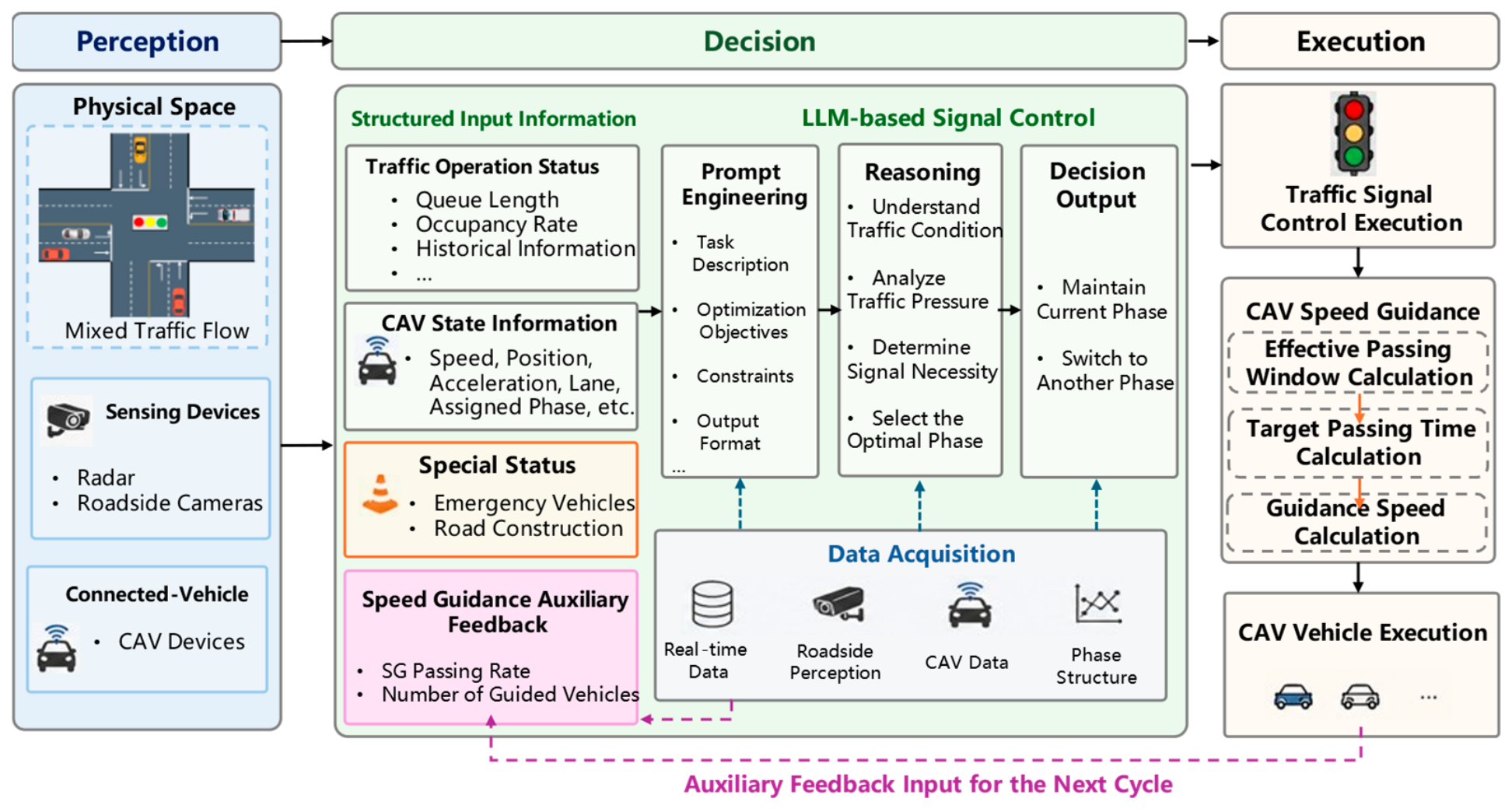
To address these limitations, this study develops an LLM-driven signal control method for urban signalized intersections under mixed traffic flow. The main contributions of this study are threefold:

• An LLM-enabled signal control framework for mixed traffic. Real-time traffic-state perception and customized prompt engineering are integrated to organize multisource traffic information and guide the LLM in generating safe, feasible, and executable phase-control decisions.
• Coordinated signal control and CAV speed guidance. A CAV speed-guidance algorithm is incorporated into the control framework, allowing vehicle speeds to be adjusted according to signal states and traffic conditions, thereby improving coordination between signal timing and vehicle operations.
• Adaptability to regular and special traffic scenarios. The proposed framework is evaluated using five matched random seeds under different CAV penetration rates, emergency-vehicle priority, road-construction constraints, multiple traffic-demand levels, and perception-noise conditions. Parameter-sensitivity and runtime experiments further examine the effects of the decision interval and speed-guidance range, together with the availability of timely LLM actions and deadline-triggered fallback operations.

The remainder of this paper is organized as follows. Section 2 introduces the preliminaries and formulates the signal-control problem. Section 3 presents the proposed LLM-driven control framework, including traffic-state perception, prompt engineering, phase decision-making, online fallback operation, and CAV speed guidance. Section 4 describes the simulation environment, experimental scenarios, comparison methods, statistical protocol, and robustness and sensitivity experiments. Section 5 reports the results under different CAV penetration rates, analyzes the microscopic effects of speed guidance, and evaluates emergency-vehicle priority, road-construction constraints, traffic-demand variation, perception noise, parameter sensitivity, and online computational responsiveness. Section 6 summarizes the findings, limitations, and future research directions.

2. Preliminaries

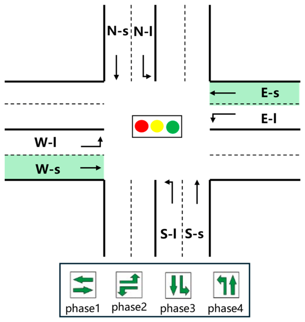
This study formulates traffic signal control at a single intersection as a discrete-time sequential decision-making problem. Let the decision step of the signal controller be Delta T. At each decision time t, the perception layer obtains the intersection traffic state, and the decision layer converts it into structured input. The LLM then outputs a phase control action under the given constraints. Based on the sensitivity analysis, Delta T = 20 is adopted in the remaining experiments as a compromise between traffic performance and online action availability.

Assume that the intersection has m controllable signal phases. The state information input to the LLM at the t-th decision time can be expressed as

$$S_t=\{B,P_t,X_t,H_t,C_t,V_t,S_{t-1}^{\mathrm{guide}}\}$$

(1)

where $B$ denotes the basic intersection information, including approaches, number of lanes, phase structure, and the corresponding permitted traffic movements; $P_t$ denotes the current signal phase state, including the current phase number, elapsed duration of the current phase, remaining green time, and whether it is in the yellow light stage; $X_t$ denotes the current traffic operation state; $H_t$ denotes the historical traffic information state; $C_t$ denotes the traffic control constraint information; $V_t$ denotes the CAV state information; $S_{t-1}^{\mathrm{guide}}$ denotes the previous-cycle CAV speed guidance feedback information.

Where the current traffic operation state $X_t$ can be further expressed as

$$X_t=\{x_{m,t}\mid m=1,2,\cdots ,M\}$$

(2)

$$x_{m,t}=(o_{m,t},q_{m,t},i_{m,t},n_{m,t})$$

(3)

where $o_{m,t}$ is the occupancy of the lane corresponding to phase $m$; $q_{m,t}$ is the queue length of the lane corresponding to phase $m$; $i_{m,t}$ is the inactive time of phase $m$; $n_{m,t}$ is the number of detected vehicles at the approach corresponding to phase $m$ during the current decision cycle.

The historical traffic state $H_t$ is used to reflect traffic variation trends and can be expressed as

$$H_t=\{X_{t-k},X_{t-k+1},\dots ,X_{t-1}\}$$

(4)

The traffic control constraint information $C_t$ can be expressed as

$$C_t=\{g_{min},g_{max},y,\mathsf{\Omega },R_t,E_t\}$$

(5)

where $g_{min}$ is the minimum green time; $g_{max}$ is the maximum green time; $y$ is the yellow light time; $\mathsf{\Omega }$ is the set of phase conflict constraints; $R_t$ is the road construction state, including affected lanes, construction duration, etc.; $E_t$ is the emergency vehicle state, including the lane of the emergency vehicle, the corresponding signal phase, etc.

For CAV states, assume that there are $N_t^{\mathrm{CAV}}$ CAVs, then:

$$V_t={\{v_{c,t},d_{c,t},a_{c,t},l_{c,t},p_{c,t}\}}_{c=1}^{N_t^{\mathrm{CAV}}}$$

(6)

where $v_{c,t}$ is the speed of the $c$th CAVs; $d_{c,t}$ is the distance from the vehicle to the stop line or intersection exit; $a_{c,t}$ is the vehicle acceleration; $l_{c,t}$ is the lane occupied by the vehicle; $p_{c,t}$ is the signal phase corresponding to the vehicle.

In terms of the action space, the phase control action output by the LLM is defined as

$$a_t\in A_t=\{keep,switch(p_j)\}$$

(7)

where $keep$ indicates maintaining the current phase, $switch(p_j)$ indicates switching to the target phase $p_j$. If a phase-switching action is selected, the minimum green time, yellow light transition, and phase conflict constraints must be satisfied; if maintaining the current phase is selected, the maximum green time constraint must be satisfied. Therefore, the actual executable action set can be expressed as

$$A_t^{valid}=\{a_t\mid a_t\in A_t, C_t(a_t)=1\}$$

(8)

where $C_t(a_t)=1$ indicates that action $a_t$ satisfies the traffic control constraints at the current moment; otherwise, the action is not executable.

Based on the above definitions, the LLM signal control process can be expressed as

$$a_t=f_{LLM}(S_t,\stackrel{⏜}{P},A_t^{valid})$$

(9)

where $f_{LLM}(.)$ denotes the decision function jointly formed by the large language model and prompt engineering; $\stackrel{⏜}{P}$ is the prompt-engineering template, which constrains the LLM to reason according to the traffic control task, information acquisition rules, phase safety constraints, and specified output format. Unlike traditional optimization algorithms, the LLM does not directly solve a closed-form optimal control equation, but performs comprehensive judgment under structured traffic state inputs and control-rule constraints to generate executable phase control actions. Equation (9) should be interpreted as an interface-level representation of a black-box conditional policy rather than a white-box analytical model of the LLM. The internal token-level assessment and decision trade-offs remain opaque.

3. Methodology

As a new type of transportation system that integrates the physical world and the digital world, the T-CPS optimizes traffic operation through real-time data interaction and intelligent decision-making. The autonomous operation of a traffic signal control system can be described as a closed loop involving information collection, information transmission, decision-making, and control execution [43]. Studying intersection control optimization algorithms from the T-CPS perspective is of great significance for improving traffic operation efficiency and traffic safety on the road section.

The method proposed in this paper takes the LLM as the decision-making core. The perception layer obtains intersection traffic states; information such as traffic operation state, CAV state, and special event state is organized into structured inputs; and executable phase control actions are generated under traffic control constraints. Unlike direct phase switching based on rules, the LLM performs comprehensive reasoning over multisource traffic information under prompt engineering constraints to judge the main traffic pressure at the current intersection, potential congestion trends, and the necessity of phase switching.

Based on the foregoing problem formulation, an LLM-based signal control framework for mixed traffic flow is developed, as illustrated in Figure 1. The framework comprises three layers: (1) a perception layer that collects and preprocesses intersection traffic, CAVs, and special-event information; (2) a decision layer in which the LLM, guided by task-specific prompts and traffic-control constraints, analyzes the structured state input and selects a feasible phase control action; and (3) an execution layer that implements the selected action in the signal controller.

3.1. Control Method Framework

3.1.1. Perception Layer

From the T-CPS perspective, the perception layer of this control method serves as the core hub for interaction between information space and physical space. It obtains traffic state information from physical space and uploads the information data to the cloud server through the Internet of Vehicles, providing real-time and accurate data support for subsequent signal control reasoning in the decision layer.

The information obtainable by the perception layer mainly includes the following two categories:

(1)

Vehicle information: CAVs transmit parameters such as acceleration, speed, position, distance to the stop line, and the number of approaching vehicles to the perception layer in real-time through onboard sensors and V2X communication technology. HVs, by contrast, can only provide local traffic state information through fixed sensors. In addition, the perception layer can obtain information about emergency vehicles at the intersection.

(2)

Intersection information: including intersection structure, number of lanes, traffic signal phases, phase-movement mapping, signal inactive time, occupancy, queue length, and other information.

3.1.2. Decision Layer

Under T-CPS, the cloud server obtains traffic state information through the Internet of Vehicles. Combining this traffic information, the decision layer of the control method uses the LLM as the core engine and customized prompt engineering as the driving mechanism. It integrates multisource data from physical space, domain knowledge, and auxiliary decision-making algorithms to generate real-time signal control decisions that comply with traffic rules, optimize traffic efficiency, and adapt to complex scenarios.

The customized prompt engineering adopted in this paper guides the LLM to reason out signal control decisions that meet the requirements and strictly control the output format and structure by designing and adjusting the instruction input to the LLM. Among them, Chain of Thought (CoT), as the core reasoning strategy, guides the model to decompose complex signal control problems step by step, further improving the logic and accuracy of the output and enabling the LLM to better realize practical value. Details are provided in Section 3.2.

This study focuses on a four-leg intersection, as shown in Figure 2. The decision layer receives traffic information transmitted by the perception layer. The approaches of the intersection are named east (E), west (W), south (S), and north (N), and vehicle movements are named through (s) and left turn (l).

The LLM reasons and deliberates based on the above multi-source traffic information and determines the signal phase for the next control cycle within each control step. In this paper, the control step is set to 20 s; that is, the phase selection for the next cycle is completed during the previous control cycle, the phase control action is executed at the beginning of the current cycle, and CAV speed guidance is carried out based on the currently determined green phase. The speed guidance part is detailed in Section 3.3.

To prevent the online reasoning time of the LLM from affecting the real-time execution of signal actions, a rolling decision mechanism one cycle in advance is adopted. During the t-th control cycle, the controller completes data acquisition, prompt construction, LLM reasoning, action parsing, and safety verification based on the current traffic state, generating a candidate phase action for the (t + 1)-th control cycle. When the (t + 1)-th control cycle begins, the system does not need to wait for LLM reasoning again but directly executes the phase action that has been cached and verified in the previous cycle. Therefore, the single LLM reasoning time and tool invocation time mainly affect whether the next cycle action can be prepared on time and do not block the signal execution already determined for the current cycle. If an LLM response timeout occurs or the output action fails the safety verification during actual operation, the controller maintains the current phase to ensure continuity and safety of signal control. Nevertheless, LLM-based online control remains subject to network-dependent inference latency, response variability, and potentially invalid or hallucinated outputs. Therefore, candidate actions are restricted to the predefined feasible phase set and verified before execution; late or invalid responses trigger a deterministic fallback that maintains the current phase.

CAV speed guidance and signal action execution occur in the same control execution cycle. Specifically, when the (t + 1)-th cycle begins to execute the phase action determined in the t-th cycle, the speed guidance module calculates the guidance speed according to the current actual green light state, remaining green time, queue dissipation time, and CAV state. If the phase action requires a yellow light transition, speed guidance is not executed during the yellow light stage; instead, it is calculated based on the effective green window after the target green light is actually activated. Therefore, speed guidance is not executed in the next-next cycle; rather, it is executed after the target phase actually enters the passable green stage. Its guided pass rate is then used as feedback input for subsequent LLM decision cycles.

The overall procedure of the proposed method is summarized in Algorithm 1.

Algorithm 1 LLM-driven signal control with CAV speed guidance

Require: traffic environment E, DeepSeek-V4-Flash model πθ, phase set Φ,

action set At, phase-action map Mapt, constraints Ct, guidance range Dguide

1: Initialize E, cached action â0, guidance record DCAV ← ∅, feedback ηguidep,0 ← 0

2: for each control cycle t = 0, 1, …, T do

3:  Execute cached and verified action ât

4:  Observe St = {B, Pt, Xt, Ht, Ct, Vt, Sguidet−1}

5:  Build Atvalid = {at | at ∈ At, Ct(at) = 1} and input xt = {St, Mapt, Atvalid}

6:  Query and parse DeepSeek-V4-Flash: (ãt+1, et) ← Parse(πθ(xt))

7:  if ãt+1 ∈ Atvalid then ât+1 ← ãt+1

8:  else ât+1 ← Fallback(current phase)

9:  end if

10:   Identify green movements Gt from ât

11:   if CAV guidance is enabled and ât is green then

12:    for each CAV c satisfying 0 < dc,t ≤ Dguide and pc,t = p do

13:    Get CAV state {lc,t, dc,t, vc,t, ac,t, pc,t}

14:    Estimate queue-dissipation time Rdisc,t

15:    Compute Weffc,t = [t + ΔTstartp + Rdisc,t, t + ΔTstartp + Gp − Δtsafe]

16:    Let Weffc,t = [teffs, teffe]

17:    Compute Tfeasiblec,t = {τ ∈ [teffs, teffe]

18:       amin ≤ ac,t(τ) ≤ amax, vmin ≤ vc,t(τ) ≤ vmax}

19:    if Tfeasiblec,t ≠ ∅ then

20:       Compute tarrc,t = t + dc,t / max(vc,t, ε)

21:       Select t*c,t = arg min over τ ∈ Tfeasiblec,t of |τ − tarrc,t|

22:       Set T*c,t = t*c,t − t

23:       Compute vguidec,t, aguidec,t, v*c,t

24:       Set vcmdc,t = min(vguidec,t, vsafec,t)

25:    else

26:       Set vcmdc,t using a deceleration-waiting or stopping strategy

27:    end if

28:    Apply vcmdc,t and store the command in DCAV

29:    end for

30:    Update ηguidep,t

31:   else

32:    Set Sguidet ← Sguidet−1

33:   end if

34: end for

35: return actions â and CAVs speed commands vcmd

3.1.3. Execution Layer

Under T-CPS, the control strategy of the decision layer is issued to the execution layer through the Internet of Vehicles to operate the traffic signal phases in physical space.

Table 1. LLM reasoning results.

… decision: Phase-2 explanation: There are no CAVs or emergency vehicles at the intersection, and traffic conditions on all road sections are normal. The inactive time of Phase-2 is 95.0 s, close to the threshold of 100 s, so release should be prioritized. In addition, the occupancies of the left-turn lanes included in Phase-2 (E-l and W-l) are 6% and 10.5%, respectively, which are relatively high; in particular, the occupancy of E0-l exceeds 10%. Although the left-turn lane of Phase-4 (S-l) has a higher occupancy (17%), its inactive time is 46.0 s and has not yet reached the threshold for urgent release. Therefore, selecting Phase-2 can effectively relieve phase congestion that is about to reach the threshold while balancing the needs of other phases. decision: Phase-4 explanation: There are no CAVs or emergency vehicles at the intersection, and traffic conditions on all road sections are normal. The currently active phase is Phase-2, whose inactive time is 0 s. The inactive times of the other phases are Phase-1: 23.0 s, Phase-3: 46.0 s, and Phase-4: 69.0 s. Phase-4 has relatively high occupancy (S-l: 22.98%) and no road construction. Considering the historical occupancy data (‘S-l’: ‘17%’, ‘S-s’: ‘4.5%’, …), selecting Phase-4 can relieve the continuously increasing traffic pressure in that direction. …

shows the results of large language model reasoning for two adjacent control steps.

3.2. Prompt Engineering

This paper selects the CoT strategy, ensuring reasoning depth suitable for dynamic traffic scenarios while also considering real-time requirements. The core of CoT is to decompose complex problems into several smaller and more manageable subproblems. Complex signal control tasks are serialized into multiple subproblems, guiding the model to perform evolutionary reasoning and gradually derive the final control strategy. This paper provides part of the prompt engineering, as shown in

Table 2. Example of prompt engineering.

You are acting as an AI signal controller to relieve intersection congestion under mixed traffic flow. Please strictly observe the following: Clarify the basic content of the signal control task. Interpret the structured traffic-state information supplied by the program. Compare the candidate phases using the supplied observations and decision rules, and select one available phase action. Return the selected phase to the execution program, which applies the signal action and performs CAV speed guidance when enabled. ## Structured traffic-state input - Intersection movement layout: {movement_info} - Signal phase structure: {phase_info} - Explicit phase–action–movement mapping: {phase_action_map} - Current signal phase: {current_phase} - Phase-level traffic-state observations: {phase_state} - {historical_data} - {inactive_time} - {cav_guidance_context} Each entry in phase_state contains: - action_index: the integer index of the candidate phase. - decision: the corresponding Phase-N action. - phase_name: the phase label in the signal phase structure. - movements: the traffic movements served by the phase. - queue_sum: the sum of valid queued-vehicle counts for the served movements. - max_occupancy: the maximum valid occupancy among the served movements, expressed as a percentage; −1 indicates that no valid occupancy value is available. - all_accessible: whether all served movements are marked as accessible. - has_road_construction: whether any served movement has road construction. - has_emergency_vehicle: whether an emergency vehicle is detected in any served movement. Use phase_action_map to associate each candidate phase with its served movements. Do not assume that a phase index has the same meaning at different intersections ## Notes When the inactive time of a phase exceeds 100 s, you need to switch to that phase. If road construction reduces the capacity of a movement, avoid ineffective green allocation while maintaining service according to the remaining capacity. If an emergency vehicle exists, priority release is required. Right-turn lanes are outside your control scope and do not need to be considered. CAV speed guidance feedback is used only as an auxiliary reference; consider releasing the phase when the guided pass rate is too low.

.

3.3. CAV Speed Guidance

To further exploit the communicable and controllable advantages of CAVs, a CAV speed guidance mechanism is introduced based on the LLM signal control results.

3.3.1. Speed Guidance Trigger Mechanism

At the end of the previous cycle, the phase decision output by the LLM signal control module is:

$$a\in \{keep,switch(p_j)\}$$

(10)

The execution layer updates the signal state according to this decision and transmits the information to the CAV guidance module.

The phrase ‘at the end of the previous cycle’ here refers to completing the precomputation of the phase action for the (t + 1)-th cycle within the t-th control cycle. The phase action is executed at the beginning of the (t + 1)-th cycle. If the target phase requires a yellow light transition, CAV speed guidance starts after the target green light is actually activated; if the current phase is maintained, speed guidance can be calculated directly based on the current remaining green time after the (t + 1)-th cycle begins.

$$I_t^{sig}=\{p_t,G_t^{rem},Y_t,\mathsf{\Delta }{T}_p^{start},G_p\}$$

(11)

where $p_t$ is the release phase determined for this cycle; $G_t^{rem}$ is the remaining green time of the current phase; $Y_t$ is the yellow light transition time; $\mathsf{\Delta }{T}_p^{start}$ is the time from the current moment t to the formal green light activation time, taken as $Y_t$, otherwise taken as 0; $G_p$ is the available green time of the phase determined for this cycle $p_t$.

For the c-th CAV, its state information can be expressed as

$$I_{c,t}^{veh}=\{v_{c,t},d_{c,t},a_{c,t},l_{c,t},p_{c,t}\}$$

(12)

where $v_{c,t}$ is the vehicle speed, $d_{c,t}$ is the distance from the vehicle to the stop line, $a_{c,t}$ is the vehicle acceleration, $l_{c,t}$ is the lane occupied by the vehicle, $p_{c,t}$ is the signal phase corresponding to the vehicle.

When a vehicle satisfies the following conditions, speed guidance is triggered:

$$0<d_{c,t}\le D_{guide}$$

(13)

and

$$p_{c,t}=p_t$$

(14)

where $D_{guide}$ is the length of the speed guidance area. If the vehicle is far from the stop line or its corresponding phase has no possibility of release in the short term, the vehicle follows the original car-following model without speed intervention.

3.3.2. Queue Dissipation Time Estimation

After the green light is activated, queued vehicles on the approach are released one by one at the saturation flow rate. Therefore, determining whether a CAV can pass through the intersection continuously requires estimating the remaining dissipation time of the queued vehicles ahead of it.

Because this paper assumes that only CAVs can provide vehicle-level state information, while ordinary vehicles do not provide individual-vehicle position and speed data, it is impossible to directly identify every vehicle ahead of a CAV. The detector provides the queue length of lane l $q_{l,t}$, and the number of queued vehicles can be approximated as follows, rounded upward:

$$N_{l,t}^q=⌈{\displaystyle \frac{q_{l,t}}{l_{veh}+s_0}}⌉$$

(15)

where $l_{veh}$ is the average vehicle length, $s_0$ is the average headway in the queued state.

Because the CAV distance to the stop line $d_{c,t}$ is known, the number of queued vehicles ahead of the CAVs can be estimated according to the positional relationship between the CAVs and the queue area:

$${\widehat{N}}_{c,t}^{front}=\left\{\begin{array}{ll}\min \left(N_{l,t}^q,⌊{\displaystyle \frac{d_{c,t}}{l_{veh}+s_0}}⌋\right),\hfill & d_{c,t}\le q_{l,t}\hfill \\ N_{l,t}^q,\hfill & d_{c,t}>q_{l,t}\hfill \end{array}\right.$$

(16)

Let the saturation discharge headway be $h_s$ and the green light start-up lost time be $t_l$, then the remaining queue dissipation time corresponding to the CAVs is:

$$R_{c,t}^{dis}={\delta }_{p,t}{t}_l+h_s{\widehat{N}}_{c,t}^{front}$$

(17)

where ${\delta }_{p,t}$ is the start-up loss correction coefficient. When the phase has not yet been activated, or when the green light has just been activated and queued vehicles have not yet completed start-up, ${\delta }_{p,t}$ = 1; when the green light has already been activated, and the start-up loss has occurred, ${\delta }_{p,t}$ = 0 to avoid repeatedly counting the start-up loss time.

3.3.3. Effective Passing Window Considering Queue Dissipation

The passage of a CAV depends not only on whether the signal is green, but also on whether the queued vehicles ahead have been released. Therefore, this paper modifies the original green window into an effective passing window that considers queue dissipation.

If the CAV corresponding phase $p_{c,t}$ is consistent with the release phase already determined for this cycle $p_t$, then its effective passing window is:

$$W_{c,t}^{eff}=\begin{array}{l}[t+\mathsf{\Delta }{T}_{p_t}^{start}+R_{c,t}^{dis},\hfill \\ t+\mathsf{\Delta }{T}_{p_t}^{start}+G_p-\mathsf{\Delta }{t}_{safe}]\hfill \end{array}$$

(18)

where $\mathsf{\Delta }{t}_{safe}$ is the safety margin at the end of the green time.

3.3.4. Feasibility of Speed Guidance

Let the effective passing window of the CAVs be:

$$W_{c,t}^{eff}=[t_s^{eff},t_e^{eff}]$$

(19)

For any candidate passing time $\tau \in W_{c,t}^{eff}$, the travel time from the current position to the stop line is:

$$T=\tau -t$$

(20)

If the vehicle adjusts its speed with uniform acceleration, the required acceleration is:

$$a_{c,t}(\tau )={\displaystyle \frac{2(d_{c,t}-v_{c,t}T)}{T^2}}$$

(21)

The corresponding speed is:

$$v_{c,t}(\tau )=v_{c,t}+a_{c,t}(\tau )T$$

(22)

Therefore, the feasible set of passing times that satisfy the speed and acceleration constraints can be expressed as

$$T_{c,t}^{feasible}=\begin{array}{l}\{\tau \in [t_s^{eff},t_e^{eff}]\mid a_{min}\le a_{c,t}(\tau )\le a_{max},\hfill \\ v_{min}\le v_{c,t}(\tau )\le v_{max}\}\hfill \end{array}$$

(23)

If:

$$T_{c,t}^{feasible}\ne Ø$$

(24)

then the CAVs can pass continuously through the intersection within the effective green window under vehicle dynamic constraints; otherwise, the vehicle should execute a deceleration, waiting, or stopping strategy.

To reduce speed fluctuation, this paper preferentially selects the feasible passing time closest to the vehicle’s natural arrival time. The vehicle’s natural arrival time is:

$$t_{c,t}^{arr}=t+{\displaystyle \frac{d_{c,t}}{max(v_{c,t},\epsilon )}}$$

(25)

The target passing time is:

$$t_{c,t}^{*}=\arg {\min }_{\tau \in T_{c,t}^{\mathrm{feasible}}}\left|\tau -t_{c,t}^{\mathrm{arr}}\right|$$

(26)

If the natural arrival time is earlier than the effective passing window, the vehicle should decelerate appropriately; if the natural arrival time is later than the effective passing window, the vehicle needs to accelerate appropriately. If the acceleration or speed constraints cannot be satisfied, the vehicle needs to wait or stop.

3.3.5. Calculation of Guidance Speed and Acceleration

After determining the target passing time $t_{c,t}^{*}$, the target travel time from the current position to the stop line is:

$$T_{c,t}^{\ast }=t_{c,t}^{\ast }-t$$

(27)

The corresponding average guidance speed is:

$${\overline{v}}_{c,t}^{guide}={\displaystyle \frac{d_{c,t}}{T_{c,t}^{\ast }}}$$

(28)

The guidance acceleration is:

$$a_{c,t}^{guide}={\displaystyle \frac{2(d_{c,t}-v_{c,t}{T}_{c,t}^{\ast })}{{(T_{c,t}^{\ast })}^2}}$$

(29)

The corresponding target terminal speed is:

$$v_{c,t}^{\ast }=v_{c,t}+a_{c,t}^{guide}{T}_{c,t}^{\ast }$$

(30)

The vehicle dynamic constraints must also be satisfied:

$$a_{min}\le a_{c,t}^{guide}\le a_{max}$$

(31)

$$v_{min}\le v_{c,t}^{\ast }\le v_{max}$$

(32)

When the above two equations are satisfied, the vehicle operates according to the calculated guidance acceleration and target speed. If they are not satisfied, the speed adjustment within the current effective passing window is infeasible, and the vehicle should decelerate to a stop.

At the same time, the actual vehicle operation must still satisfy car-following and safe-distance constraints. The final control speed can be expressed as

$$v_{c,t}^{cmd}=min({\overline{v}}_{c,t}^{guide},v_{c,t}^{\mathrm{safe}})$$

(33)

where $v_{c,t}^{\mathrm{safe}}$ is the safe speed determined by the car-following model or safe-distance constraint. Through the above processing, CAVs can make their arrival time at the stop line match the effective green window, considering queue dissipation as closely as possible while satisfying safe car-following constraints.

3.3.6. CAV Speed Guidance Feedback

To strengthen the information linkage between signal control and vehicle speed guidance, this paper introduces the CAV speed guidance pass rate as auxiliary feedback information and uses it as a supplementary input state for the LLM in the next control cycle.

$${\eta }_{p,t}^{guide}={\displaystyle \frac{N_{p,t}^{pass}}{N_{p,t}^{guide}+\epsilon }}$$

(34)

where ${\eta }_{p,t}^{guide}$ is the CAV speed guidance pass rate; $N_{p,t}^{guide}$ is the number of CAVs participating in speed guidance for phase p during cycle t; $N_{p,t}^{pass}$ is the number of CAVs that successfully pass the stop line after speed guidance during cycle t.

Equation (34) is used to evaluate the execution outcome of the speed-guidance commands issued for phase p during the preceding control interval. The feedback is regarded as reliable only when at least two CAVs received speed guidance. A one-vehicle sample is ignored because its guidance pass rate can only be either zero or one and therefore provides insufficient evidence for signal adjustment.

For a reliable sample, the desired outcome is a ${\eta }_{p,t}^{\mathrm{guide}}$ value approaching one, indicating that all guided CAVs pass the stop line within the evaluation interval. A value below one indicates that at least one of the guided CAVs did not complete the intended passage during that interval. The feedback does not directly determine the next signal action. Emergency-vehicle priority, movement accessibility, safety constraints, current traffic demand, and downstream capacity remain the primary decision factors. When two or more feasible phases exhibit comparable real-time traffic demand, a guidance pass rate below one, calculated from a reliable sample, gives the previously evaluated phase secondary priority, provided that the phase remains accessible.

4. Experiments

4.1. Simulation Environment Construction

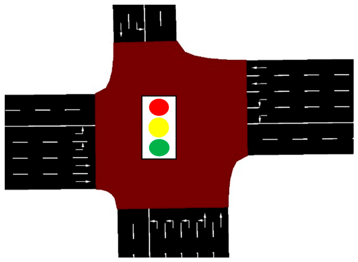
This paper builds the simulation environment using the SUMO microscopic simulation platform (version 1.23.1). To verify the actual effect of the signal control method, an intersection in Nanning is selected as the case study, and the intersection scenario is shown in Figure 3. The north–south approaches are 200 m long, the east–west approaches are 250 m long, and the first 150 m before each approach is set as the speed guidance detection area. Traffic volume is collected by roadside devices deployed by the traffic police. The collection time is the evening peak period on 28 April 2025, with a collection interval of 5 min. Part of the collected data is shown in

Table 3. Traffic volume collection table. (using 17:00–17:05 as an example).

Approach	Vehicles	Through Movement Proportion
East approach	68	0.88
West approach	62	0.67
North approach	43	0.36
South approach	136	0.21

. To characterize the differentiated driving features of CAVs and HVs in mixed traffic flow, this paper uses the IDM model to describe the car-following behavior of HVs and the CACC model to describe the car-following behavior of CAVs.

In addition, in the experiment, the speed guidance parameters are set as follows: the saturation headway h_s is 2 s, the green-light start-up lost time $t_l$ is 2 s, the green-end safety margin $\mathsf{\Delta }{t}_{safe}$ is 1 s, the maximum acceleration is 3 m/s², the maximum deceleration is −2 m/s², the average vehicle length $l_{veh}$ is 5 m, and the maximum guidance speed $v_{max}$ is 18 m/s.

To simplify the research scenario, focus on the core problem, and provide prerequisites for the subsequent simulation scheme design, the following assumptions are made for the simulation scenario:

(1)

The main experiments assume ideal V2X communication without transmission delay or packet loss. Therefore, they represent an upper-bound communication condition. A separate sensitivity experiment examines uncertainty in the queue-length and lane-occupancy observations supplied to the LLM.

(2)

The impacts of pedestrians and non-motorized vehicles are not considered.

(3)

Because the intersection has dedicated right-turn lanes and vehicles are not affected by signal control, this paper does not consider the impact of right-turn vehicles.

4.2. Simulation Scheme Design

The evaluation consists of a regular mixed-traffic scenario and two non-recurrent operational scenarios involving emergency-vehicle priority and road-construction constraints. Additional experiments examine different traffic-demand levels, perception noise, and the sensitivity of the decision interval and CAV speed-guidance range. For each evaluated method and experimental configuration, five independent runs were conducted using random seeds 1–5. Within each comparison, the same traffic seed and route file were used across the evaluated methods. Each run covered 2000 s of simulated traffic operation, and the results are reported as the run-level mean and sample standard deviation. The evaluation indicators include average waiting time (AWT), average fuel consumption (AFC), and average number of stops (ANS). Emergency-vehicle average waiting time (EV-AWT) is additionally evaluated in the emergency-vehicle scenario.

4.2.1. Regular Scenario

The regular scenario is used to analyze the effect of changes in CAV penetration rate on signal control performance. This study sets the CAV penetration rates to 0, 0.25, 0.5, 0.75, and 1, respectively. CAVs can upload information such as vehicle speed, position, acceleration, lane, and corresponding phase to the perception layer through V2X communication. This scenario is used to test the control performance of the proposed method under different degrees of CAV information availability.

4.2.2. Emergency Vehicle Scenario

The emergency vehicle scenario is used to simulate special vehicles with priority-passage needs, such as ambulances and fire engines. This study introduces a small number of emergency vehicles into the baseline traffic flow and assumes that their arrival times and arrival directions are randomly generated. During the entire simulation process, emergency vehicles account for approximately 1% of all vehicles.

When an emergency vehicle is detected entering the influence area of the intersection, information such as its lane, corresponding phase, and position is input to the LLM signal controller as priority control constraints.

4.2.3. Road Construction Scenario

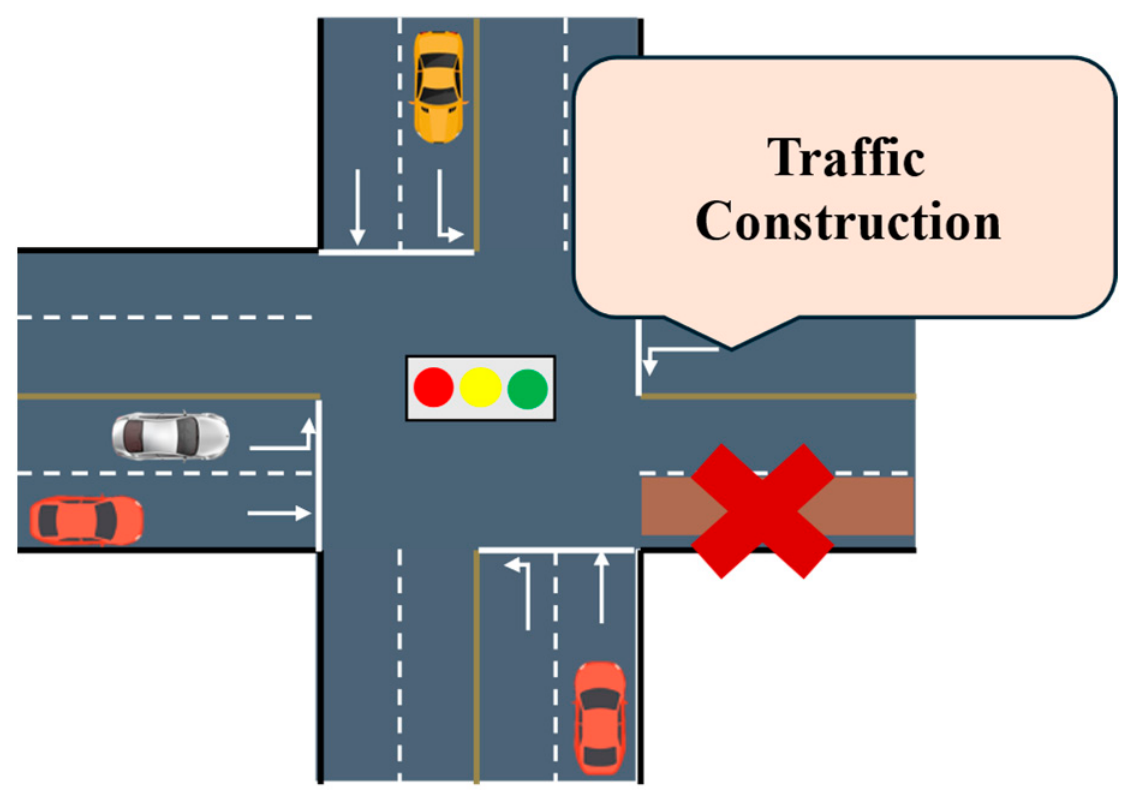
The road construction scenario, illustrated in Figure 4, is designed to simulate a localized reduction in downstream capacity. From 600 to 800 s of the simulation, one lane of the eastbound exit link is completely closed due to construction. During this period, the capacity of the affected exit decreases, which may cause queues to propagate upstream and influence traffic operations in other directions. The signal controller is therefore required to adjust the green time adaptively according to the real-time queue conditions, reduce ineffective green allocation to the affected movement, and maintain adequate service for the unaffected movements.

4.2.4. Traffic-Demand Variation Experiment

To evaluate whether the performance of the proposed method depends on a single traffic-demand pattern, three demand levels were considered: low, baseline, and high traffic demand. The baseline profile was derived from the observed peak traffic demand at the investigated intersection. The low-demand profile was approximately 75% of the baseline demand, whereas the high-demand profile was approximately 1.12 times the baseline demand. Because the baseline already represents peak-hour conditions, the high-demand scenario was designed to simulate a temporary traffic surge caused by large-scale events or other unusual demand disturbances. The turning proportions, intersection geometry, vehicle parameters, and controller settings were kept unchanged across the three demand levels. Experiments were conducted at CAV penetration rates of 0% and 50%, using five matched random seeds for each configuration. The results are reported as the run-level mean and standard deviation.

4.2.5. Perception-Noise Robustness Experiment

To approximate the traffic-state perception uncertainty that may arise from roadside sensors, vehicle detectors, and data-aggregation processes in real-road environments, a perception-noise sensitivity experiment was conducted under the regular traffic scenario. The CAV penetration rate, decision interval, and speed-guidance range were fixed at 50%, Delta T = 20 s, and D_guide = 150 m, respectively. Three perception-noise levels, sigma = 0, 0.10, and 0.20, were considered. Five matched traffic seeds and identical route files were used across all noise conditions.

For each movement-level queue-length or lane-occupancy observation x supplied to the LLM, the noisy observation was generated as

$$\tilde{x}=\mathrm{clip}\left[x(1+\sigma \epsilon )\right],\hspace{1em}\hspace{1em}\hspace{1em}\hspace{1em}\epsilon ~N(0,1).$$

(35)

where $\tilde{x}$ denotes the traffic-state observation perceived by the controller, $\epsilon$ is a standard Gaussian random variable, and $\sigma$ determines the intensity of perception noise.

The perturbation was applied only to the aggregate movement-level queue-length and occupancy information supplied to the LLM. It did not alter the physical traffic state in SUMO, the ground-truth data used to calculate the evaluation metrics, individual CAV states, or vehicle dynamics.

To quantify the actual magnitude of the observation perturbation, the relative mean absolute error (RMAE) was calculated separately for movement-level queue length and lane occupancy as

$${\mathrm{RMAE}}_x={\displaystyle \frac{{\displaystyle \sum _{t,m}\left|{\tilde{x}}_{m,t}-x_{m,t}\right|}}{{\displaystyle \sum _{t,m}|}{x}_{m,t}|}},\hspace{1em}\hspace{1em}\hspace{1em}\hspace{1em}x\in \{q,o\}.$$

(36)

where m and t denote the traffic movement and observation time, respectively; q represents queue length; and o represents lane occupancy.

4.2.6. Parameter-Sensitivity and Online-Response Experiments

The sensitivity experiments are conducted under the regular traffic scenario with a CAV penetration rate of 50% and matched traffic-demand seeds. For the decision-interval experiment, Delta T is set to 10, 15, and 20 s, while $D_{\mathrm{guide}}$ is fixed at 150 m. For the guidance-range experiment, $D_{\mathrm{guide}}$ is set to 0, 50, 100, 150, and 200 m while Delta T is fixed at 20 s. In addition to AWT, AFC, and ANS, the experiments report the proportion of usable responses returned within Delta T, and the fallback-action frequency.

To further examine the trade-off between bounded online responsiveness and potential traffic performance, the operational full LLM configuration was compared with a deadline-disabled reference. In the deadline-disabled reference, the simulator waited for the complete API response and accepted valid actions returned after the operational deadline. The same model, prompt, controller parameters, route files, and five traffic seeds were used in both configurations. Because physical traffic would continue evolving while waiting for a delayed response, the deadline-disabled configuration is treated only as an offline reference rather than an online-deployable controller.

4.2.7. Ablation Experiment Design

To identify the respective contributions of the functional prompt blocks, three ablated variants of the proposed method were constructed. LLM without Phase-level state representation (PSR) removes the phase-level structured representation and supplies the same underlying queue, occupancy, accessibility, detector status, and emergency vehicle observations at the movement level. The LLM must therefore associate these observations with the candidate phases through the phase–action map. An LLM without the Operational-Constraint Block (OCB) removes the operational-constraint information and associated decision rules concerning emergency-vehicle priority and movement accessibility under road-construction-induced capacity restrictions. LLM without output structure constraints (OSC) removes the explicit output-structure constraints while retaining the traffic-state information and decision rules. The complete method, denoted as Full LLM, retains all three functional blocks. The configurations of the full framework and its ablation variants are summarized in

Table 4. Configurations of the proposed framework and its component-ablation variants.

Method	Structured Traffic State Input	PSR	OCB	OSC	CAV Speed Guidance
Full LLM	√	√	√	√	√
LLM w/o PSR	√	—	√	√	√
LLM w/o OCB	√	√	—	√	√
LLM w/o OSC	√	√	√	—	√

.

All variants used the same LLM, model parameters, traffic routes, CAV speed-guidance algorithm, decision interval, and random seeds. Except for the functional block being examined, the remaining prompt components and controller settings were unchanged. The experiments were conducted under the regular traffic scenario and the two special scenarios using five matched traffic seeds. Results are reported as the run-level mean and standard deviation.

4.2.8. Coupling of Baseline Signal Controllers with CAV Speed Guidance

To distinguish the contribution of LLM-based phase decision-making from that of the CAV speed-guidance module, the same signal-consistent speed-guidance algorithm was coupled with four adaptive baseline controllers: SOTL, Max-pressure, PPO-based, and UniTSA. Each baseline retained its original state representation, phase-selection policy, trained parameters, and action space. After the baseline selected a signal phase, the speed-guidance module calculated the effective passage window and generated feasible speed recommendations for CAVs within the guidance range. No LLM reasoning or prompt-based decision process was introduced into these baseline controllers. The experiments were conducted under the regular traffic scenario at CAV penetration rates of 0%, 25%, 50%, 75%, and 100%, using five matched traffic seeds for each configuration. The decision interval and guidance range were fixed at ΔT = 20 s and D_guide = 150 m, respectively.

4.3. Comparison Methods

To verify the effectiveness of the proposed LLM signal control method, this paper selects the following methods for comparison:

(1)

Fixed Time Control (FTC): a traditional signal control method that uses the fixed cycle of the real intersection.

(2)

Single-intersection Webster: calculates the optimal signal cycle and green split for each phase according to the vehicle arrival rate of each approach at the intersection, with the aim of minimizing average vehicle delay.

(3)

Self-Organizing Traffic Light control (SOTL): the signal light autonomously decides whether to switch phases according to the current phase and competing phases, giving priority to high-demand directions and reducing vehicle waiting time.

(4)

Max-pressure: an adaptive traffic signal control method based on pressure balancing. It balances the queue lengths of adjacent intersections by optimizing the pressure of each phase, reduces oversaturation risk, and ultimately maximizes the overall throughput of the road network.

(5)

PPO-based: an RL-based traffic signal control method. The state space is represented by lane-level occupancy, and the action space is restricted to selecting a signal phase from a predefined set of feasible phase schemes. The reward function is defined as the negative average vehicle waiting time.

(6)

UniTSA [44]: a universal reinforcement-learning framework for V2X traffic signal control. Following the original study, UniTSA uses a junction matrix to represent movement-level traffic flow, maximum and average occupancy, movement attributes, lane numbers, current- and next-phase signal states, and minimum-green satisfaction. The latest $K=8$ junction-matrix snapshots are stacked as the input state, corresponding to approximately 40 s of historical traffic information under the original 5 s action interval. Its action space follows the original keep-or-change design, and its reward is the normalized negative average queue length.

The principal training and implementation settings of the PPO-based and UniTSA controllers are summarized in

Table 5. Training and implementation settings of the learning-based baseline controllers.

Method	Parameter	Setting
PPO-based	Training steps	300,000
	Parallel environments	6
	Episode duration	2000 s
	Rollout length	5000 steps per environment
	Batch size	64
	Optimization epochs	10
	Learning-rate schedule	Linear decay
	Feature dimension	32
UniTSA	Training steps	800,000
	Rollout length	512
	Batch size	128
	Optimization epochs	5
	Learning-rate schedule	Linear decay
	Discount factor	0.99
	GAE coefficient	0.95
	Clipping range	0.20

. Both controllers were trained only under the regular traffic scenario, and their trained parameters were frozen during all subsequent evaluations, including the emergency-vehicle, road-construction, and CAV speed-guidance coupling experiments.

(7)

LLM: the proposed signal control method uses DeepSeek-V4-Flash through the DeepSeek API (base URL: https://api.deepseek.com; API model identifier: deepseek-v4-flash), accessed between 15 and 30 August 2026. Requests were issued using the LangChain Chat OpenAI client (version 1.3.14). The model was specified by its API identifier rather than a pinned snapshot.

Through prompt engineering, this method integrates intersection operation states, CAV information, and special scenario constraints to generate real-time phase control decisions satisfying traffic control constraints and combines a speed guidance algorithm to achieve collaborative optimization. The same original prompt template was used across all experimental scenarios. Under the provider’s default thinking mode, temperature and top-p settings have no effect. The model parameters were not trained or fine-tuned for any experimental scenario. Responses exceeding the deadline or failing output verification were discarded, and the controller maintained the current phase as the fallback action.

(8)

LLM-noSG: the signal control method proposed in this paper without speed guidance, compared with the LLM method.

To ensure a consistent evaluation protocol, the PPO-based and UniTSA controllers were trained only under the regular traffic scenario, and their parameters were frozen during the emergency-vehicle and road-construction tests. The parameters of DeepSeek-V4-Flash were not trained or fine-tuned for any experimental scenario; instead, a fixed prompt template was used to interpret real-time traffic observations and operational constraints. Therefore, the special-scenario experiments evaluate training-free responsiveness to non-recurrent conditions rather than superiority over RL controllers specifically retrained for each event.

5. Experimental Results

5.1. Analysis of Results in the Regular Scenario

5.1.1. Performance Analysis Under Different CAV Penetration Rates

To verify the control performance of the proposed LLM signal control method under different CAV penetration rates, this paper sets the CAV penetration rates to 0, 0.25, 0.5, 0.75, and 1 and selects multiple methods for comparative experiments. The evaluation indicators include average waiting time, average fuel consumption, and average number of stops.

As shown in

Table 6. Evaluation indicators under different penetration rates. Mean ± sample SD (n = 5).

Penetration Rate	Method	AWT (s)	AFC (g)	ANS
0	Fixed-time	96.26 ± 1.68	126 ± 1	4.44 ± 0.10
	Webster	92.37 ± 4.39	120 ± 1	4.58 ±0.41
	SOTL	66.17 ± 3.62	97 ± 2	2.40 ± 0.15
	Max-pressure	63.07 ± 2.89	98 ± 2	2.49 ± 0.15
	PPO-based	53.47 ± 4.11	101 ±1	2.01 ± 0.12
	UniTSA	45.21 ± 3.28	75 ± 2	2.12 ± 0.32
	LLM	50.42 ± 4.84	89 ± 3	2.10 ± 0.20
0.25	Fixed-time	102.32 ± 4.59	120 ± 1	3.78 ± 0.12
	Webster	95.01 ± 5.02	109 ± 2	2.98 ± 0.06
	SOTL	64.37 ± 4.62	97 ± 3	1.90 ± 0.11
	Max-pressure	64.69 ± 3.06	96 ± 2	2.12 ± 0.06
	PPO-based	54.81 ± 4.76	107 ± 2	2.05 ± 0.18
	UniTSA	48.90 ± 3.97	76 ± 2	2.26 ± 0.20
	LLM-noSG	49.17 ± 7.89	84 ± 6	2.35 ± 0.25
	LLM	48.31 ± 10.84	81 ± 11	2.09 ± 0.39
0.5	Fixed-time	92.09 ± 2.34	107 ± 5	3.80 ± 0.19
	Webster	83.30 ± 2.43	104 ± 5	3.02 ± 0.41
	SOTL	61.83 ± 3.48	95 ± 4	1.89 ± 0.10
	Max-pressure	58.76 ± 3.26	94 ± 3	2.21 ± 0.04
	PPO-based	52.32 ± 3.71	100 ± 2	2.12 ± 0.30
	UniTSA	44.58 ± 5.10	77 ± 4	1.9 ± 0.04
	LLM-noSG	43.31 ± 6.31	79 ±5	2.24 ± 0.32
	LLM	37.60 ± 8.50	76 ± 9	1.52 ±0.34
0.75	Fixed-time	90.35 ± 2.28	98 ± 2	3.32 ± 0.15
	Webster	80.73 ± 4.92	95 ± 5	2.23 ± 0.24
	SOTL	53.31 ± 4.76	85 ± 5	1.72 ± 0.05
	Max-pressure	51.12 ± 3.50	86 ± 4	2.15 ± 0.06
	PPO-based	47.72 ± 3.75	85 ± 3	2.33 ± 0.15
	UniTSA	40.20 ± 4.15	79 ± 3	1.75 ± 0.42
	LLM-noSG	38.80 ± 5.20	71 ± 5	1.70 ± 0.30
	LLM	33.51 ± 4.46	67 ± 3	1.17 ± 0.12
1	Fixed-time	87.44 ± 11.07	114 ±2	2.30 ± 0.42
	Webster	77.87 ± 7.83	99 ± 3	2.11 ± 0.32
	SOTL	48.00 ± 2.67	80 ± 2	1.42 ± 0.09
	Max-pressure	49.23 ± 3.11	75 ± 2	1.10 ± 0.06
	PPO-based	41.92 ± 5.65	74 ± 2	1.23 ± 0.34
	UniTSA	32.25 ± 4.25	70 ± 1	1.19 ± 0.20
	LLM-noSG	28.90 ± 5.75	68 ± 3	1.23 ± 0.12
	LLM	22.76 ± 3.54	69 ± 4	1.16 ± 0.15

, with the increase in CAV penetration rate, the average waiting time of the proposed LLM method shows an obvious overall downward trend. When the CAV penetration rate is 0, the average waiting time of the LLM method is 50.42 s. When the penetration rate increases to 0.25, 0.5, 0.75, and 1, the average waiting time decreases to 48.31 s, 37.60 s, 33.51 s, and 22.76 s, respectively. As the proportion of CAVs increases, the system can obtain more sufficient information on vehicle speed, position, and arrival trends, allowing the LLM to more accurately judge the traffic demand of each phase during phase decision-making. At the same time, the signal control result can further act on the CAV speed guidance module, thereby reducing ineffective waiting before the stop line.

When the CAV penetration rate is 0, the average waiting time of the LLM method is 50.42 s, lower than those of Fixed-time, Webster, SOTL, Max-pressure, and PPO-based, but higher than the 45.21 s of UniTSA. This indicates that even without introducing CAV speed guidance, the LLM method can still make relatively effective phase selections based on multisource data. However, because CAV state and speed guidance information are absent at this time, the collaborative advantage of the LLM has not yet been fully exerted, and therefore it does not achieve the best result compared with UniTSA. Since there are no CAVs that can receive speed guidance in this scenario, no LLM-noSG comparative experiment is needed.

When the CAV penetration rate increases to 0.25, the average waiting time of the LLM method is 48.31 s. This corresponds to reductions of 52.79%, 49.15%, 24.95%, 25.32%, 11.86%, and 1.21% relative to Fixed-time, Webster, SOTL, Max-pressure, PPO-based, and UniTSA, respectively. However, the difference from UniTSA is small compared with the run-to-run variation and should therefore be interpreted as comparable performance rather than a decisive advantage.

When the CAV penetration rate reaches 0.75, the average waiting time of the LLM method decreases to 33.51 s, which is 29.78% and 16.64% lower than PPO-based and UniTSA, respectively. Compared with low-penetration scenarios, the advantage of the LLM method over LLM-noSG also further expands at this stage, indicating that as the proportion of CAVs increases, vehicle state information becomes more sufficient and the collaborative effect between signal control results and CAV speed guidance becomes more evident.

When the CAV penetration rate is 1, the average waiting time of the LLM method decreases to 22.76 s, the lowest value among all methods. Compared with Fixed-time, Webster, SOTL, Max-pressure, PPO-based, and UniTSA, the average waiting time of the LLM method decreases by 73.97%, 70.77%, 52.58%, 53.77%, 45.71%, and 29.43%, respectively. Meanwhile, compared with LLM-noSG, the average waiting time of the LLM method decreases by 21.25%, and the average number of stops decreases from 1.23 to 1.16. These results show that in a fully CAV environment, the proposed method can fully use vehicle speed, position, phase state, and queue information to realize collaborative optimization between signal control and vehicle speed guidance, thereby reducing intersection delay.

The nonlinear improvement at high CAV penetration rates may be associated with heterogeneous car-following interactions and the increasing occurrence of consecutive CAV vehicle pairs. Previous studies have similarly reported that the traffic-flow benefits of CACC or CAV control may remain limited at low penetration rates but become more pronounced after reaching a moderate or high penetration threshold [45,46,47,48]. At low penetration rates, isolated speed-guided CAVs remain constrained by surrounding HVs, whereas at high penetration rates, consecutive groups of controllable CAVs can more consistently adjust their arrival times to the available green window. Nevertheless, differences in the car-following models and vehicle-dynamics parameters of CAVs and HVs may also contribute to this trend.

5.1.2. Time-Space Trajectory Analysis

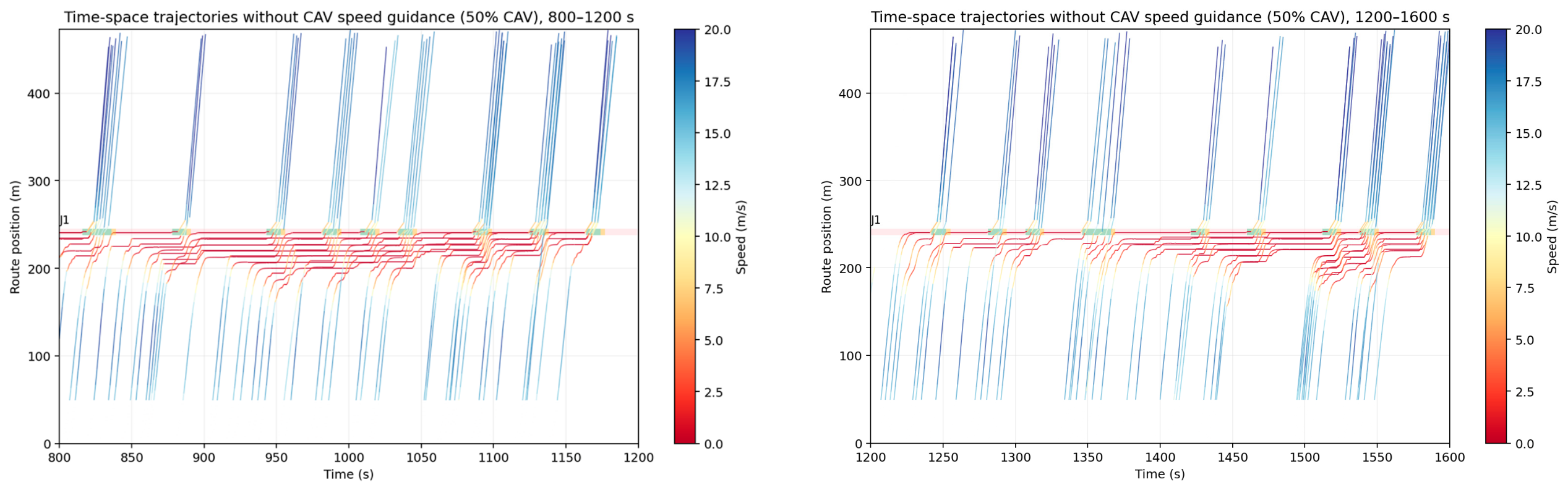
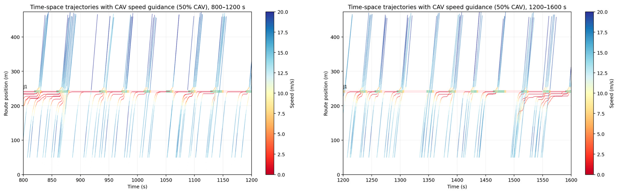
To examine the microscopic impact of CAV speed guidance under the proposed signal control framework, Figure 5 and Figure 6 present the time-space trajectories of all eastbound through vehicles traveling from the western approach to the eastern exit link through J1 under a 50% CAV penetration rate. Here, J1 denotes the focal four-leg signalized intersection in the study network. The vertical axis represents the cumulative route position, with the J1 stop line located at approximately 250 m. Trajectory colors denote instantaneous vehicle speed, ranging from red for low speeds to blue for high speeds, while the horizontal signal bands indicate the signal phases at J1. Without CAV speed guidance, many vehicles exhibit extended low-speed or stopped trajectories upstream of the stop line, indicating recurrent queuing and deceleration before the intersection. With speed guidance, vehicle trajectories generally show smoother approach patterns and shorter low-speed segments in several signal cycles, particularly during the 800–1200 s interval. However, low-speed queues are still observed during periods of relatively high demand.

5.1.3. Effects on Traffic Efficiency and Speed Stability

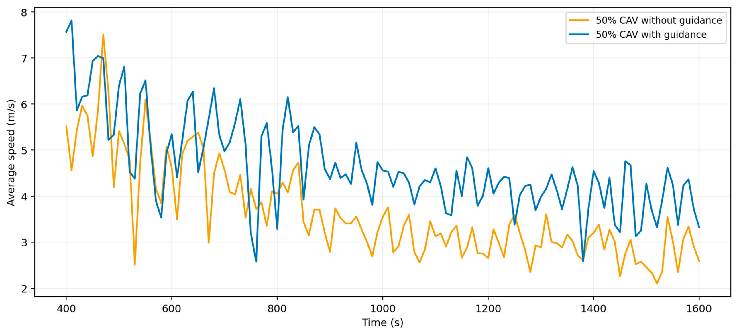
Figure 7 compares the average vehicle speed in the study intersection network, aggregated at 10 s intervals from 400 to 1600 s, under a 50% CAV penetration rate. Although both profiles fluctuate because of signal phase transitions and queue dynamics, the CAV’s speed-guidance case maintains a higher average speed during most intervals, particularly after 850 s. This indicates that speed guidance helps CAVs adjust their approach speeds to better match the available green time, thereby reducing unnecessary braking.

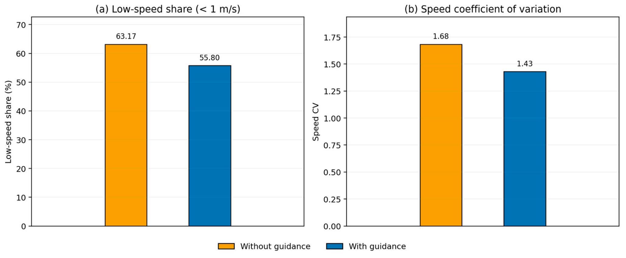
To further quantify the effects of CAV speed guidance, four indicators are evaluated: average speed, low-speed share, speed coefficient of variation (CV), and total inbound throughput. The low-speed share is defined as the proportion of vehicle state samples with speeds below 1 m/s, reflecting the prevalence of queuing and stopping. The speed CV, calculated as the ratio of speed standard deviation to mean speed, is used to measure relative speed stability.

Figure 8 compares the traffic performance with and without CAV speed guidance. Compared with the no-guidance case, CAV speed guidance increases the average speed from 3.48 to 4.58 m/s, corresponding to an improvement of 31.4%. The low-speed share decreases from 63.17% to 55.80%, a reduction of 7.36 percentage points. In addition, the speed CV decreases from 1.683 to 1.430, indicating a 15.0% improvement in relative speed stability. The total inbound throughput increases from 1100 to 1135 vehicles, representing an increase of 3.2%. These quantitative results corroborate the time series observations, indicating that CAV speed guidance reduces low-speed operation and improves traffic efficiency under the proposed signal control framework.

5.2. Analysis of Results in the Emergency Vehicle Scenario

To further verify the applicability of the proposed LLM-based signal control method in special traffic-demand scenarios, an emergency-vehicle priority-passage scenario was evaluated at CAV penetration rates of 0%, 25%, 50%, 75%, and 100%.

Table 7. AWT under different CAV penetration rates in the emergency-vehicle scenario. Mean ± sample SD (n = 5).

Method	Penetration Rate
	0	0.25	0.5	0.75	1
Fixed-time	98.97 ± 2.21	102.54 ± 4.55	92.93 ± 2.35	90.40 ± 2.72	87.44 ± 11.07
Webster	90.58 ± 3.45	94.61 ± 6.01	89.36 ± 1.16	87.99 ± 7.06	84.63± 7.83
SOTL	63.20 ± 5.21	65.63 ± 2.87	60.92 ± 3.59	55.10 ± 2.55	48.00 ± 2.6
Max-pressure	59.20 ± 4.69	61.92 ± 2.77	57.63 ± 4.51	55.33 ± 3.56	49.23 ± 3.11
PPO-based	55.32 ± 3.75	53.36 ± 8.21	51.46 ± 8.87	48.64 ± 3.51	44.29 ± 1.96
UniTSA	48.45 ± 3.50	49.25 ± 7.32	48.94 ± 1.50	47.03 ± 3.00	40.81 ± 4.20
LLM-noSG	-	47.86 ± 3.45	45.67 ± 4.24	44.27 ± 3.14	36.51 ± 2.42
LLM	46.80 ± 5.01	45.61 ± 4.82	42.88 ± 3.71	41.97 ± 5.72	31.19 ± 3.76

and

Table 8. EVAWT under different CAV penetration rates in the emergency-vehicle scenario. Mean ± sample SD (n = 5).

Method	Penetration Rate
	0	0.25	0.5	0.75	1
Fixed-time	91.11 ± 16.05	95.55 ± 20.68	86.16 ± 17.25	85.87 ± 21.70	78.85 ± 12.51
Webster	90.41 ± 19.15	93.70 ± 24.05	84.48 ± 16.43	80.84 ± 18.16	77.28 ± 22.02
SOTL	61.53 ± 8.15	61.44 ± 13.09	58.30 ± 13.50	47.61 ± 5.91	42.32 ± 3.89
Max-pressure	57.01 ± 12.06	58.22 ± 16.30	55.12 ± 15.63	52.25 ± 9.46	48.22 ± 10.32
PPO-based	50.97 ± 11.13	47.95 ± 10.08	45.38 ± 8.42	40.97 ± 11.13	42.58 ± 7.27
UniTSA	55.80 ± 17.97	49.24 ± 12.29	45.35 ± 17.10	41.79 ± 13.45	38.68 ±16.98
LLM-noSG	-	20.45 ± 3.98	21.18 ± 2.74	17.04 ± 5.49	16.96 ± 5.37
LLM	20.34 ± 2.00	19.82 ± 4.45	18.80 ± 3.02	16.94 ± 4.47	15.80 ± 3.02

report the overall AWT and EVAWT, respectively.

As detailed in Section 4.3, the PPO and UniTSA checkpoints and controller parameters were kept fixed in the emergency-vehicle experiments, without scenario-specific retraining or tuning.

Table 7 and Table 8 show that the proposed method achieves the lowest numerical AWT and EVAWT at all five CAV penetration rates. As the CAV penetration rate increases from 0% to 100%, the AWT of the proposed method decreases from 46.80 s to 31.19 s, while its EV-AWT decreases from 20.34 s to 15.80 s. At 0% penetration, the EVAWT of the proposed method is 60.09–77.68% lower than those of the six comparison methods. At 50% penetration, introducing CAV speed guidance reduces AWT from 45.67 s to 42.88 s and EV-AWT from 21.18 s to 18.80 s compared with LLM-noSG. These results indicate that the proposed controller can consistently incorporate emergency-vehicle priority information while benefiting from increasing connected-vehicle availability.

In summary, the proposed LLM signal control method can effectively identify emergency vehicle priority-passage demand and reduce emergency vehicle waiting time through dynamic signal phase adjustment while maintaining good operating efficiency for ordinary vehicles. Compared with traditional timed control and rule-based control methods, the LLM can use structured prompt engineering to comprehensively reason over traffic states, historical trends, and emergency vehicle information.

5.3. Analysis of Results in the Road Construction Scenario

To evaluate the robustness of the proposed method under abnormal traffic-organization conditions, the road-construction scenario was examined at CAV penetration rates of 0%, 25%, 50%, 75%, and 100%. The AWT results are reported in

Table 9. AWT under different CAV penetration rates in the road construction scenario. Mean ± sample SD (n = 5).

Method	Penetration Rate
	0	0.25	0.5	0.75	1
Fixed-time	102.84 ± 5.51	103.22 ± 4.30	99.57 ± 2.87	96.05 ± 3.75	93.57 ± 7.98
Webster	99.46 ± 8.12	100.43 ± 4.40	95.18 ± 6.31	94.30 ± 7.74	90.14 ± 4.82
SOTL	65.68 ± 10.48	61.96 ± 8.73	60.18 ± 10.11	56.63 ± 7.37	52.84 ± 5.62
Max-pressure	66.53 ± 6.30	60.22 ± 3.63	62.77 ± 3.90	59.48 ± 4.10	55.74 ± 4.99
PPO-based	64.73 ± 6.77	60.83 ± 9.68	55.49 ± 6.84	53.24 ± 6.72	42.45 ± 2.58
UniTSA	62.65 ± 5.72	57.00 ± 4.24	51.03 ± 5.39	51.91 ± 5.41	43.12 ± 4.26
LLM-noSG	-	53.78 ± 6.35	47.98 ± 3.45	46.16 ± 6.73	41.07 ± 5.89
LLM	59.22 ± 6.12	52.46 ± 4.56	45.74 ± 2.51	40.54 ± 5.76	35.35 ± 4.19

. The construction-induced downstream-capacity restriction changes the traffic pressure across different approaches and phases, thereby providing a test of the controllers’ adaptability to non-recurrent operational constraints. The same frozen-parameter protocol described in Section 4.3 was applied to the road construction experiments.

Table 9 shows that the proposed LLM method obtains the lowest numerical AWT at all five CAV penetration rates. Its AWT decreases from 59.22 s at 0% penetration to 35.35 s at 100% penetration, corresponding to an overall reduction of 40.31%. At 50% penetration, CAV speed guidance further reduces AWT from 47.98 s for LLM-noSG to 45.74 s for LLM. Although the magnitude of the improvement varies across penetration rates, the overall results indicate that connected-vehicle information and signal-consistent speed guidance improve the controller’s ability to respond to construction-induced downstream-capacity restrictions.

5.4. Ablation and Component-Contribution Analysis

5.4.1. Prompt-Functional Ablation Under Regular Traffic

Table 10. Prompt-functional ablation results under regular traffic. Mean ± sample SD (n = 5).

Method	AWT (s)	Returned Within ΔT (%)	Fallback-Action Frequency (%)	Mean Inference Time (s)
Full LLM	37.60 ± 8.50	85.76 ± 7.49	13.25 ± 7.67	8.32 ± 0.86
LLM w/o PSR	42.81 ± 6.85	90.21 ± 3.87	8.28 ± 3.58	8.12 ± 0.71
LLM w/o OCB	43.77 ± 11.64	80.82 ± 8.07	17.94 ± 8.52	7.98 ± 1.74
LLM w/o OSC	68.68 ± 16.56	69.84 ± 9.10	27.73 ± 8.11	12.31 ± 1.08

compares the contributions of the three prompt-functional blocks under regular traffic. The full LLM achieves the lowest AWT while maintaining a relatively high proportion of responses returned within Delta T. Removing PSR slightly reduces the mean inference time and increases the timely return rate, but results in higher AWT. This indicates that the phase-level representation contributes primarily to decision quality rather than computational speed: aggregating movement-level observations into phase-aligned queue and occupancy indicators reduces the need for the LLM to reconstruct the relationship between traffic demand and candidate phases.

The poorer traffic-control performance of LLM w/o OCB may be partially associated with its lower returned within Delta T rate and correspondingly higher fallback-action frequency compared with Full LLM. When a valid action is unavailable before the decision deadline, the controller retains the current phase as the fallback action. Although this policy guarantees executable online control, frequent fallback operation may prevent timely phase adjustment in response to evolving queues. The degradation should not, however, be attributed exclusively to response availability, because removing OCB also eliminates explicit operational-feasibility and priority cues that may help structure the decision process. Since these constraints are not continuously activated under regular traffic, their specific contribution is further examined under the emergency-vehicle and road-construction scenarios in Section 5.4.2.

Removing OSC produces the clearest deterioration in both online responsiveness and traffic performance. Its mean inference time increases to 12.31 s, while the proportion of responses returned within Delta T decreases to 69.84% and the fallback-action frequency rises to 27.73%. Without explicit output-format constraints, the model is more likely to produce unnecessarily extended or structurally inconsistent responses, reducing the availability of executable actions within the decision interval. Overall, the results indicate that PSR mainly supports phase-selection quality, OCB supplies operational-feasibility guidance, and OSC is particularly important for obtaining timely and executable online control actions.

5.4.2. Operational-Constraint Ablation Under Special Scenarios

To further examine the contribution of the OCB, Full LLM and LLM w/o OCB were evaluated under the emergency-vehicle and road-construction scenarios at a CAV penetration rate of 50%. Five matched traffic seeds and identical scenario settings were used. The results are presented in

Table 11. Operational-constraint ablation results under emergency-vehicle and road-construction scenarios. Mean ± sample SD (n = 5).

Scenario	Method	AWT (s)	EAAWT (s)	Returned Within ΔT (%)	Fallback-Action Frequency (%)
Emergency vehicle	Full LLM	42.88 ± 3.71	18.80 ± 3.02	90.06 ± 4.34	9.19 ± 5.04
	LLM w/o OCB	47.44 ± 13.36	42.31 ± 8.98	79.77 ± 7.06	18.74 ± 6.95
Road construction	Full LLM	45.74 ± 2.51	-	83.35 ± 4.34	15.41 ± 3.60
	LLM w/o OCB	74.97 ± 20.21	-	78.29 ± 3.43	19.24 ± 3.43

.

Removing the OCB produced particularly evident deterioration in the scenario-specific indicators. In the emergency-vehicle scenario, the overall AWT increased by 10.63%, while EV-AWT increased by 125.05%. The much larger change in EV-AWT indicates that queue and occupancy information alone may not ensure timely service for a low-frequency emergency movement. The explicit emergency-priority information and associated decision rules in the OCB enable the LLM to identify the affected phase and treat its release requirement as a primary constraint.

In the road-construction scenario, removing the OCB increased AWT by 63.91%. Without explicit information and instructions concerning construction-induced movement accessibility and capacity restrictions, the controller may continue to allocate green time mainly according to observed queue and occupancy. This can result in ineffective release toward the capacity-constrained movement and aggravate upstream queuing.

5.4.3. Cross-Controller Contribution of CAV Speed Guidance

To separate the contribution of CAV speed guidance from that of signal decision-making,

Table 12. AWT comparison of signal controllers with and without CAV speed guidance. Mean ± sample SD (n = 5).

Method	CAV Penetration	Baseline AWT (s)	Baseline + SG AWT (s)	Improvement
SOTL	0%	66.17 ± 3.62	66.17 ± 3.62	0%
	25%	64.37 ± 4.62	49.90 ± 5.00	22.48%
	50%	61.83 ± 3.48	49.59 ± 2.15	19.80%
	75%	53.31 ± 4.76	50.76 ± 17.56	4.78%
	100%	48.00 ± 2.67	43.13 ± 15.77	10.15%
Max-pressure	0%	63.07 ± 2.89	63.07 ± 2.89	0%
	25%	64.69 ± 3.06	52.37 ± 2.14	19.04%
	50%	58.76 ± 3.26	54.52 ± 1.97	7.22%
	75%	51.12 ± 3.50	51.01 ± 4.56	0.22%
	100%	49.23 ± 3.11	54.95 ± 8.92	−11.62%
PPO-based	0%	53.47 ± 4.11	53.47 ± 4.11	0%
	25%	54.81 ± 4.76	53.05 ± 17.52	3.21%
	50%	52.32 ± 3.71	39.53 ± 4.93	24.45%
	75%	47.72 ± 3.75	35.48 ± 3.68	25.65%
	100%	41.92 ± 5.65	30.78 ± 2.11	26.57%
UniTSA	0%	45.21 ± 3.28	45.21 ± 3.28	0%
	25%	48.90 ± 3.97	46.03 ± 2.02	5.87%
	50%	44.58 ± 5.10	43.02 ± 0.95	3.50%
	75%	40.20 ± 4.15	38.21 ± 2.69	4.95%
	100%	32.25 ± 4.25	34.81 ± 4.20	−7.94%
LLM	0%	50.42 ± 4.84	50.42 ± 4.84	0%
	25%	49.17 ± 7.89	48.31 ± 10.84	1.75%
	50%	43.31 ± 6.31	37.60 ± 8.50	13.18%
	75%	38.80 ± 5.20	33.51 ± 4.46	13.63%
	100%	28.90 ± 5.75	22.76 ± 3.54	21.25%

compares each controller with and without the same guidance module at matched CAV penetration rates. Improvement denotes the percentage reduction in AWT relative to the corresponding controller without guidance; a negative value indicates increased waiting time. At 0% penetration, the paired results are identical because no vehicle receives speed guidance.

The results show that the effect of speed guidance depends on both the underlying controller and CAV penetration. SOTL obtains positive mean improvements at all nonzero penetration rates, although its benefit is greater at 25% and 50% than at higher penetration rates. For Max-pressure, the improvement decreases from 19.04% at 25% penetration to almost zero at 75%, before becoming negative at 100%. PPO-based control benefits from guidance at all tested nonzero penetration rates, with larger reductions in AWT from 50% penetration onward. UniTSA obtains modest improvements between 25% and 75%, but its mean AWT increases by 7.94% at full penetration. These comparisons demonstrate that speed guidance is not an independently additive component whose benefit necessarily increases with penetration.

For the proposed framework, speed guidance reduces the mean AWT at every nonzero penetration rate, with the reduction increasing from 1.75% at 25% penetration to 21.25% at full penetration. LLM with guidance achieves the lowest mean AWT among the evaluated configurations from 50% to 100% penetration. The LLM controller already provides comparatively low AWT without guidance over this range, while the addition of guidance produces a further reduction. The observed performance should therefore be attributed to the combination of traffic-responsive LLM phase selection and signal-consistent CAV speed adjustment, rather than to either component alone.

A possible explanation for the controller-dependent results is that speed guidance changes CAV arrival times and consequently modifies the queue and occupancy patterns observed by the signal controller. These changes are beneficial when the resulting arrivals remain aligned with subsequent green service but may be counterproductive when the signal logic responds inadequately to the modified traffic distribution. In the evaluated UniTSA configuration, the policy determines whether to maintain the current phase or advance to the next phase in a predefined sequence, rather than freely selecting any target phase. This restricted action structure may limit its ability to realign green service with guidance-induced arrival changes at high penetration. Similarly, pressure- or occupancy-responsive controllers may react to spatial traffic-state changes introduced by guided vehicle trajectories.

Related non-monotonic interactions were also reported by Maadi et al. [37], who observed that the queue-length ratio of their RL controller with speed guidance increased in several higher-penetration configurations. They attributed this partly to the broad guidance coverage and low minimum advisory speed used in their study, which could generate queues behind guided CAVs. Although their guidance strategy and performance measures differ from those adopted here, their findings likewise indicate that increasing the number of guided vehicles does not necessarily produce a monotonic improvement in intersection-level performance.

5.5. Performance Under Different Traffic-Demand Levels

Table 13. Average waiting time under different traffic-demand levels at 0% CAV penetration. Mean ± sample SD (n = 5).

Method	Demand
	Low	Baseline	High
Fixed-time	41.96 ± 4.26	96.26 ± 1.68	115.39 ± 7.85
Webster	38.51 ± 5.60	92.37 ± 4.39	103.71 ± 7.38
SOTL	33.87 ± 3.56	66.17 ± 3.62	83.03 ± 2.78
Max-pressure	35.64 ± 1.64	63.07 ± 2.89	78.08 ± 5.22
PPO-based	30.84 ± 1.18	53.47 ± 4.11	75.05 ± 4.73
UniTSA	29.53 ± 6.86	45.21 ± 3.28	68.04 ± 4.96
LLM	29.20 ± 6.64	50.42 ± 4.84	72.03 ± 10.36

and

Table 14. Average waiting time under different traffic-demand levels at 50% CAV penetration. Mean ± sample SD (n = 5).

Method	Demand
	Low	Baseline	High
Fixed-time	40.15 ± 2.34	92.09 ± 2.34	127.28 ± 6.11
Webster	34.78 ± 3.64	83.30 ± 2.43	101.43 ± 5.47
SOTL	29.19 ± 2.02	61.83 ± 3.48	72.63 ± 6.33
Max-pressure	32.84 ± 2.39	58.76 ± 3.26	70.77 ± 2.93
PPO-based	25.00 ± 1.37	52.32 ± 3.71	65.67 ± 7.78
UniTSA	24.13 ± 1.18	44.58 ± 5.10	60.28 ± 4.82
LLM-noSG	24.91 ± 2.01	43.31 ± 6.31	60.35 ± 10.25
LLM	24.01 ± 1.20	37.60 ± 8.50	55.98 ± 6.72

compare the average waiting time of the evaluated methods under low, baseline, and high traffic-demand levels at CAV penetration rates of 0% and 50%, respectively. The baseline demand represents the observed peak-hour traffic condition, the low-demand profile is approximately 75% of the baseline demand, and the high-demand profile represents a temporary traffic surge. All values are reported as the run-level mean and standard deviation over five independent runs.

As expected, the average waiting time generally increases as traffic demand rises. At 0% CAV penetration, the AWT of the proposed LLM method increases from 29.20 s under low demand to 50.42 s under baseline demand and 72.03 s under high demand. The LLM method achieves the lowest numerical AWT under low demand. Under baseline and high demand, however, UniTSA obtains lower AWT values of 45.21 s and 68.04 s, respectively, compared with 50.42 s and 72.03 s for the LLM method. This result indicates that when no CAV information or speed-guidance capability is available, the proposed method remains competitive but does not consistently outperform the reinforcement-learning baseline.

At 50% CAV penetration, the proposed LLM method achieves the lowest numerical AWT under all three demand levels, with values of 24.01 s, 37.60 s, and 55.98 s under low, baseline, and high demand, respectively. Compared with Fixed-time control, these values correspond to reductions of 40.20%, 59.17%, and 56.02%. Compared with UniTSA, the reductions are 0.50%, 15.66%, and 7.13%, respectively. The difference under low demand is relatively small compared with the run-to-run variability, whereas clearer advantages are observed under baseline and high demand.

Comparing the two penetration levels, introducing 50% CAVs reduces the AWT of the proposed method by 17.77%, 25.43%, and 22.28% under low, baseline, and high demand, respectively. These results indicate that the proposed framework can use connected-vehicle information and signal-consistent speed guidance across different demand levels. Nevertheless, the AWT still rises to 55.98 s under high demand, showing that the proposed method cannot fully eliminate delay when traffic demand approaches the capacity of the intersection.

5.6. Robustness Analysis Under Perception Noise

To examine the robustness of the proposed controller to imperfect traffic-state perception, perception-noise experiments were conducted under the regular traffic scenario with a CAV penetration rate of 50%. The decision interval was fixed at Delta T = 20 s, and the CAV speed-guidance range was fixed at D_guide = 150 m. Three perception-noise levels, namely $\sigma$ = 0, 0.10, and 0.20, were considered. Five matched traffic seeds and identical route files were used under all noise conditions. The results are reported as the run-level mean and sample standard deviation in

Table 15. Performance and observation errors under different perception-noise levels. Mean ± sample SD (n = 5).

$\mathit{\sigma }$	Queue Relative MAE (%)	Occupancy Relative MAE (%)	AWT (s)	AFC (g)	ANS
0	0	0	37.60 ± 8.50	76 ± 9	1.52 ± 0.34
0.1	8.15 ± 0.30	7.90 ± 0.30	41.61 ± 5.59	74 ± 3	1.49 ± 0.10
0.2	16.25 ± 0.84	16.11 ± 0.54	48.51 ± 10.73	76 ± 6	1.59 ± 0.26

.

As the noise standard deviation increased from 0.10 to 0.20, Q-RMAE increased from 8.15% to 16.25%, while O-RMAE increased from 7.90% to 16.11%. These values confirm that the magnitude of the observation error increased approximately proportionally with the prescribed noise level. The slightly smaller relative errors than the nominal noise standard deviations are consistent with the expected absolute magnitude of zero-mean Gaussian perturbations and the clipping of physically infeasible observations.

Traffic performance exhibited moderate sensitivity to increasingly inaccurate observations. AWT increased from 37.60 s under the no-noise condition to 41.61 s at $\sigma$ = 0.10, and further to 48.51 s at $\sigma$ = 0.20. This indicates that errors in the movement-level queue and occupancy information can affect the phase-selection decisions of the LLM, particularly when the observation errors become relatively large. Nevertheless, AFC remained approximately stable across the three conditions, while ANS changed only slightly from 1.52 to 1.59. Therefore, although perception noise produced some degradation in waiting-time performance, the controller remained operational and did not exhibit abrupt deterioration in fuel consumption or stopping frequency.

5.7. Parameter Sensitivity and Online Computational Responsiveness

Increasing Delta T generally increased the proportion of usable LLM responses returned within the nominal decision interval and reduced the fallback-action frequency. Here, “Returned within Delta T” denotes the proportion of LLM calls that produced a valid control action within the nominal decision interval. Compared with Delta T = 10 s, the 20 s setting produced a similar AWT and nearly identical AFC, while reducing ANS from 2.02 to 1.52. Therefore, among the tested values, Delta T = 20 s provides the most balanced trade-off between traffic performance and online action availability. The performance variation is not strictly monotonic because changing Delta T affects not only the available inference time but also the synchronization among traffic-state sampling, phase transitions, and short-term queue evolution.

These results quantify rather than eliminate the inference-latency limitation. Any response that misses the permitted decision deadline or fails output verification is rejected and handled by the deterministic fallback before signal execution.

Table 16. Sensitivity analysis of the decision interval Delta T and online response availability. Mean ± sample SD (n = 5).

ΔT (s)	AWT (s)	AFC (g)	ANS	Returned Within ΔT (%)	Fallback-Action Frequency (%)
10	39.72 ± 10.01	76 ± 5	2.02 ± 0.21	63.89 ± 10.32	32.56 ± 9.11
15	45.54 ± 12.70	87 ± 6	2.25 ± 0.40	72.02 ± 8.99	27.22 ± 9.16
20	37.60 ± 8.50	76 ± 9	1.52 ± 0.34	85.76 ± 7.49	13.25 ± 7.67

quantifies the availability of timely LLM actions but does not directly indicate whether rejecting delayed responses affects traffic performance. Therefore, an additional deadline-disabled reference was examined at the same decision interval of Delta T = 20 s. As shown in

Table 17. Comparison of deadline-enforced and deadline-disabled LLM control under regular traffic. Mean ± sample SD (n = 5).

Method	AWT (s)	AFC (g)	ANS	Mean Inference Time (s)
Operational deadline	37.60 ± 8.50	76 ± 9	1.52 ± 0.34	8.32 ± 0.86
Deadline-disabled reference	31.48 ± 3.30	67 ± 2	1.24 ± 0.09	17.26 ± 6.81

, this reference allows the simulator to wait for and adopt valid responses returned after the operational deadline, whereas the operational configuration rejects such responses and maintains the current phase when no usable action is available before the deadline.

The deadline-disabled reference produced a lower observed AWT of 31.48 s, compared with 37.60 s under the operational deadline, but increased the mean inference time from 8.32 to 17.26 s. Thus, disabling the deadline did not make the remote API more responsive; it merely allowed delayed responses to be accepted after the operational decision window. The results suggest that deadline enforcement may forgo some potentially beneficial LLM actions, but it bounds the waiting time and prevents delayed responses from interrupting signal execution.

To further examine the sensitivity of the proposed method to the spatial coverage of CAV speed guidance, D_guide was varied from 0 to 200 m, while Delta T was fixed at 20 s and the traffic demand, CAV penetration rate, and remaining controller settings were kept unchanged. This parameter determines the upstream distance over which CAVs can receive and execute signal-consistent speed recommendations. As shown in

Table 18. Sensitivity analysis of the CAV speed-guidance range D_guide. Mean ± sample SD (n = 5).

Dguide (m)	AWT (s)	AFC (g)	ANS
0	43.31 ± 6.31	79 ± 5	2.24 ± 0.32
50	44.72 ± 7.85	78 ± 4	1.95 ± 0.45
100	38.78 ± 12.00	76 ± 9	1.89 ± 0.24
150	37.60 ± 8.50	76 ± 9	1.52 ± 0.34
200	46.16 ± 9.75	82 ± 5	2.39 ± 0.40

, extending the guidance range does not produce a monotonic improvement in traffic performance. A short guidance range leaves vehicles with limited distance for gradual speed adjustment, whereas an excessively long range may include vehicles whose arrivals do not belong to the immediate effective passage window and may consequently introduce unnecessary early interventions. The intermediate setting of 150 m was therefore retained as a deployment-oriented compromise. It provides sufficient distance for smooth speed adjustment while limiting the guidance operation to vehicles that are directly relevant to the upcoming signal cycle.

6. Conclusions

An LLM-driven intersection signal control method is proposed for mixed traffic flow. The method obtains intersection operation states, CAV state information, historical traffic information, and special-scenario information through the perception layer and uses prompt engineering to constrain the LLM to generate executable phase control decisions. A CAV speed guidance algorithm is further designed so that signal control results can affect vehicle operation, thereby realizing collaborative optimization between signal phase decision-making and CAV speed adjustment. Based on the SUMO simulation platform, scenarios with different CAV penetration rates, emergency vehicle passage, and road construction are constructed, and the proposed method is compared with Fixed-time, Webster, SOTL, Max-pressure, PPO-based, and UniTSA methods.

The results show that the proposed method has good delay-control capability, with its advantages generally becoming more evident as the availability of CAV state information increases. This improvement is associated with the coordination between LLM-based phase decision-making and CAV speed guidance, which jointly considers vehicle states, effective passage windows, and queue-dissipation conditions. Across different traffic-demand levels, the proposed method remains competitive and benefits from connected-vehicle information and speed guidance. In non-recurrent scenarios, it can incorporate emergency-vehicle priority and temporary road-construction constraints into its phase decisions without retraining the LLM parameters. The perception-noise experiments further demonstrate that the controller remains operational under imperfect queue-length and occupancy observations, although its waiting-time performance exhibits moderate sensitivity as the noise level increases. Overall, the performance gains are scenario- and metric-dependent rather than uniform under all conditions.

In addition, the limitation of this study is that the developed signal control method optimizes only a single isolated intersection and cannot guarantee overall effectiveness in a real road network. At the network level, route guidance, traffic signal optimization, and CAV trajectory planning can be integrated within a unified framework to improve overall traffic efficiency [49]. Multi-agent coordinated control with asynchronous decision cycles also provides a potential approach for coupling traffic controllers operating at different temporal and spatial scales [50]. Future work should explore multi-intersection coordination schemes. The framework also remains dependent on remote API availability and is subject to inference latency, response variability, and potentially invalid or hallucinated outputs.