Dynamic Resilience Screening of Strait of Hormuz-Induced Trade Squeeze in Global Food Supply Chain Systems

Highlights

Systems science contribution

• An ordered country–month transition model traces how a localized chokepoint shock moves through route disruption, market reallocation, household access and crop calendar production risk.
• By separating shock entry, state crossing and intervention timing, the framework locates the binding propagation layer instead of compressing resilience into a single composite score.

Main findings and implications

• In the hypothetical Hormuz stress test, trade squeeze accounts for 92.1–94.5% of modeled normalized import availability pressure, while only 39 of 161 alerted countries cross to model-Crisis or a higher internal state.
• State crossing occurs when reallocation pressure meets weak household access and delayed production risk, and intervention value falls sharply once the active breakpoint has passed.

Abstract

A maritime chokepoint shock can spread beyond the countries directly connected to the affected route. We develop a monthly resilience screening model for a hypothetical Strait of Hormuz closure that separates direct disruption, scarcity-driven trade squeeze, household access pressure and delayed production risk. Hormuz severity variants and related Red Sea, Black Sea and fertilizer node scenarios test the stability of the modeled mechanism ordering. A three-event historical panel provides a limited external consistency check, not full model validation. In the baseline Hormuz stress test, mean modeled import availability pressure ranges from 0.0023 to 0.0076 on the normalized scale during March–August 2026. Trade squeeze accounts for 92.1–94.5% of that pressure, compared with 5.5–7.9% for direct disruption. Of 161 countries entering model-Alert, 39 later enter model-Crisis or a higher internal state. Crossings concentrate where reallocation pressure coincides with weak household access and delayed production risk. Historical estimates are directionally consistent for some events, although the Suez window exhibits non-flat pre-event coefficients and is not interpreted causally. The state labels are internal thresholds, not humanitarian classifications. The model identifies which propagation layer is binding and how quickly the associated intervention window closes.

1. Introduction

Global supply chains are studied through several modeling traditions that answer different questions. System dynamics represents disruption through stocks, flows, delays and feedback, making it well suited to temporal propagation but often too aggregated to identify which trade route or importer receives the shock first [1,2]. Bullwhip models explain how ordering and information dynamics amplify variability upstream, but their focal outcome is demand and order variance rather than cross-country food access stress following a route shock [3]. Ecological and infrastructure resilience emphasize absorption and recovery [4,5], while supply chain formulations add redundancy, flexibility and continuity [6,7]. Definitions that include adaptation or transformation do not imply that every quantitative model represents structural change. Network science resolves topology and heterogeneous connectivity [8,9]; robustness and interdependence studies show how failures propagate across nodes and coupled systems [10]. These representations do not by themselves translate a route disruption into household food access.

Supply chain research has brought these traditions closer. Disruption studies relate network design and mitigation capability to impact severity [11,12]. Strategy reviews classify preparedness, response and recovery measures [13,14], whereas quantitative reviews and viability research focus on measurement and survival under prolonged disruption [15,16]. System dynamics applications make feedback and inventories explicit [17]. Maritime network studies identify route structure and infrastructure criticality [18,19], while port resilience work examines rerouting and operational continuity [20]. More recent work adds smart port coordination, chokepoint exposure and structural vulnerability analysis [21,22,23]. These approaches provide either temporal detail or network detail. Few connect route entry, market redistribution, household access and delayed agricultural production in one ordered country–month screen.

Multi-criteria, digital and organizational resilience studies broaden managerial diagnosis, but composite capability or vulnerability scores rarely identify where a disruption becomes binding. Port vulnerability analysis provides a structural diagnosis of logistics systems [24], while grain chain analysis under drought shows the value of locating critical nodes and stages [25]. These approaches inform intervention design, yet neither directly separates physical entry, importer displacement, household access and the production calendar in one transition sequence.

Food trade research provides the empirical mechanisms needed for that distinction. International trade can support dietary diversity and buffer local harvest shocks [26,27], but dependence on distant suppliers also creates exposure to correlated disruption and network fragility [28]. Resilience and teleconnection studies show that the same trade network can absorb one regional shock and transmit another [29,30,31]. Commodity network analysis identifies an efficiency–resilience trade-off [32]. Empirical studies then show heterogeneous propagation in seafood trade networks [33], and multilayer analyses extend this logic to interacting food systems and chokepoints [34,35].

Market and policy responses determine how physical disruption is distributed. Export restrictions and strategic trade policy can amplify scarcity and prices [36,37,38]. Price shocks and pandemic disruption affect countries unevenly because income and procurement conditions differ [39,40]; landed-cost heterogeneity adds exchange rate, freight and financing exposure [41]. Reserves and alternative trade arrangements can absorb part of the shock [42,43], while energy and fertilizer costs carry it into later production periods [44]. Cooperation and supply chain capabilities can reduce unilateral amplification [45,46]. Dietary outcomes and production exposure remain conditioned by trade structure and input systems [47,48], while governance and social protection shape the final food security consequence [49].

The distinction from the closest modeling traditions is summarized in

Table 1. Comparison with representative modeling approaches.

Representative Approach	Principal Result or Strength	Boundary for the Present Question	Difference in This Study
Forrester and Sterman: system dynamics [1,2]	Stocks, flows, feedback and delays explain temporal amplification and policy response.	Aggregate structures commonly provide limited resolution of route-specific entry and importer heterogeneity.	Monthly state transitions and delays are retained, but pressures are conditioned on country, commodity, route exposure and intervention timing.
Lee et al.: bullwhip model [3]	Demand processing, rationing, batching and price variation can amplify order variance upstream.	The principal outcome is order variability in a serial supply chain rather than food access stress across countries.	Amplification is represented as scarcity-driven reallocation after direct route loss, followed by separate access and production lag operators.
Buldyrev et al. on interdependent networks and Ivanov and Dolgui on viability [10,16]	Coupled failures and survival conditions show how disruption propagates through connected systems.	Structural or binary failure measures do not directly resolve prices, household access and crop calendar timing.	A fixed network is combined with continuous country–month pressures and explicit entry, crossing and intervention tasks.
Laber et al.: multilayer food production network [34]	Interacting production and trade layers transmit shocks and alter food availability across regions.	Maritime entry, scarcity allocation, household access and intervention timing are not jointly decomposed into one transition sequence.	The model attributes pressure across route entry, reallocation, access and delayed production before assigning an internal state.
Verschuur et al. and Alexander et al.: chokepoint and input cost assessments [22,44]	Route disruption and energy–fertilizer price shocks quantify large trade, production and consumption consequences.	These assessments do not use the same country–month state-crossing screen to locate the active propagation layer.	Hormuz links maritime, energy, fertilizer and food channels in one bounded case study, with mechanism ablations and timing experiments.

. The comparison focuses on the mechanism each model resolves, its principal analytical result and the layer that remains outside its boundary. It is representative rather than exhaustive.

This study links those mechanisms through an ordered resilience screen centered on a hypothetical Strait of Hormuz closure. Trade squeeze is the study’s name for scarcity-driven import pressure that remains after the direct route component has been separated. It is a modeled attribution component, not an observed market share or a claim that importer competition is a newly discovered phenomenon. Likewise, entry, crossing and breakpoint are operational labels for the timing of exposure, threshold transition and intervention opportunity. Import availability risk, household pressure and delayed production risk map to established availability, access and production lag concepts.

The contribution is therefore methodological but deliberately bounded. The model separates direct disruption from reallocation pressure, domestic access pressure and delayed production risk in a monthly country-level stress test. Related scenarios and historical event windows are used to assess whether the direction of this sequence survives changes in the entry shock. The model evaluates absorption and recovery within the represented network. It does not endogenously transform the network topology. Hormuz is the focal case because it couples maritime routing, energy prices, fertilizer inputs and crop calendars. The analysis is not a forecast of a real 2026 crisis, and the model state labels (model-Alert, model-Crisis and model-Emergency) are not IPC, FEWS NET, WFP or famine classifications.

The analysis addresses three diagnostic questions. How does a Hormuz shock enter country food systems through route exposure and absorption capacity? When does direct exposure become scarcity-driven reallocation pressure and then cross a stricter internal state threshold? Which intervention layer retains value once deployment delay is considered? These questions organize the model sequence, results and policy experiments. Because the 2026 closure is hypothetical and the historical panel is directional, they are investigated as bounded stress test questions rather than confirmatory causal hypotheses.

2. Conceptual Framework and Mathematical Formulation

The model follows the implemented screening sequence rather than a general equilibrium or route optimization system. It represents three country-level pressures: import availability risk ($IAR$), delayed production risk ($DPR$) and household access pressure ($HP$). Direct disruption and trade squeeze are separate components of $IAR$. All pressure variables are normalized to $[0,1]$, with larger values denoting stronger stress. This compact formulation removes parameters that are not used in the reported calculations and links every equation to a reported output.

2.1. System Boundary and Interpretation of Resilience

Countries are indexed by i, food groups by g and months by t. The country state is represented by

$$X_{i,t}=\left(IA{R}_{i,t},DP{R}_{i,t},H{P}_{i,t},Z_{i,t},Stat{e}_{i,t}\right),$$

(1)

where Z is the internal severity score. The monthly transition is

$$X_{t+1}=\mathcal{F}(X_t,s_t,U_t;\Theta ),$$

(2)

with scenario shock $s_t$, intervention vector $U_t$ and parameter set $\Theta$.

The network topology is fixed over each scenario. Route and supplier edges can be degraded through the scenario inputs, but new routes, modes or contracts are not selected endogenously. Resilience in this study therefore refers to absorption, survivability and recovery within the represented structure. Adaptability and transformability, which would require endogenous network reconfiguration, are outside the reported stress test. Entry, crossing and breakpoint are timing labels within this transition system, not new resilience constructs.

Let $\mathcal{C}\left(x\right)=min\{1,max(0,x\left)\right\}$ denote truncation to the unit interval. Country–food group variables are aggregated using dietary energy weights ${\phi }_{i,g}$, where ${\sum }_g{\phi }_{i,g}=1$.

2.2. Direct Disruption and Trade-Squeeze Pressure

The direct component of import pressure is

$$D_{i,g,t}=\mathcal{C}\left[{\mu }_D{s}_t{E}_{i,g}^F(0.55+0.45d_{i,g})(0.55+0.45c_{i,g})r_{i,g}\right],$$

(3)

where $E^F$ is route-related food exposure, d is food-import dependence, c is supplier concentration risk, r is the export restraint multiplier and ${\mu }_D$ scales direct disruption.

Trade squeeze is the scarcity-driven component that is not mechanically proportional to direct route exposure:

$$S_{i,g,t}=\mathcal{C}\left[{\mu }_S{f}_t(0.35+0.65d_{i,g})(0.35+0.65e_i)(0.35+0.65c_{i,g})\right],$$

(4)

where $f_t$ is the freight and fuel reallocation shock, $e_i$ is energy import dependence and ${\mu }_S$ controls reallocation strength. The multiplicative form gives the term a clear interpretation. Reallocation pressure is strongest when the system-wide freight shock meets import dependence, energy dependence and concentrated sourcing.

The resulting increment in import availability risk is

$$\Delta IA{R}_{i,g,t}=\mathcal{C}\left[(D_{i,g,t}+S_{i,g,t})(1-0.40b_{i,g}-0.15{\mathsf{\ell }}_{i,g,t})\right],$$

(5)

where b is the baseline control buffer index and ℓ is logistics support. The country-level components are

$$D_{i,t}=\sum _g{\phi }_{i,g}{D}_{i,g,t},S_{i,t}=\sum _g{\phi }_{i,g}{S}_{i,g,t}.$$

(6)

The trade squeeze attribution share reported in the Section 4 is

$$TSShar{e}_t={\displaystyle \frac{{\sum }_i{S}_{i,t}}{{\sum }_i(D_{i,t}+S_{i,t})+\epsilon }}.$$

(7)

It is a decomposition of normalized import availability pressure, not a tonnage loss or observed market share. The corresponding absolute scale is reported as the country mean

$${\overline{IAP}}_t={\displaystyle \frac{1}{N_t}}\sum _i(D_{i,t}+S_{i,t}).$$

(8)

The reported calculation does not use a softmax allocation score. Softmax, CES, auction and linear programming allocation models would require contract-level demand, bids, elasticities, shipment capacities or market-clearing constraints that are not observed consistently across countries. A gravity model can characterize baseline bilateral trade propensity, but it does not by itself determine short-run scarcity allocation across importers without additional capacity and behavioral assumptions. Equation (4) is instead a transparent reduced-form screening operator. Its strength is varied directly through ${\mu }_S=0.8,1.0,1.2$, avoiding an unsupported payment capacity coefficient.

2.3. Delayed Production and Household Access Pressures

Energy and fertilizer shocks reach later production windows through

$$\begin{array}{cc}\hfill G_{i,g,t}^E& =(0.75E_i^E+0.25p_t^E)e_i{s}_t,\hfill \end{array}$$

(9)

$$\begin{array}{cc}\hfill G_{i,g,t}^F& =(0.70E_i^{Fert}+0.30{\tilde{p}}_t^{Fert})d_i^{Fert}{\tilde{s}}_t,\hfill \end{array}$$

(10)

where tildes denote lagged monthly scenario inputs. Delayed production risk is

$$\Delta DP{R}_{i,g,t}=\mathcal{C}\left[{\mu }_P(0.45G_{i,g,t}^E+0.55G_{i,g,t}^F)(0.55+0.45h_g)K_{i,g,t}^{cal}(1-0.35{\mathsf{\ell }}_{i,g,t})\right],$$

(11)

with food group input sensitivity $h_g$ and monthly crop calendar kernel $K^{cal}$. The kernel shifts energy and fertilizer pressure across months. It does not resolve the effect of a two-week delay within a month.

Import and production pressures affect households through food and energy costs. Define

$$\begin{array}{cc}\hfill FCos{t}_{i,g,t}& =q_g(0.45+0.55d_{i,g})s_t+p_t^F(0.35+0.65d_{i,g}),\hfill \end{array}$$

(12)

$$\begin{array}{cc}\hfill ECos{t}_{i,t}& =p_t^E(0.35+0.65e_i),\hfill \end{array}$$

(13)

where $q_g$ is the food group price sensitivity and $p_t^F$ and $p_t^E$ are scenario food and energy price pressures. Household pressure increases by

$$\begin{array}{cc}\hfill \Delta H{P}_{i,g,t}=\mathcal{C}[& {\mu }_A\left(0.40FCos{t}_{i,g,t}+0.30ECos{t}_{i,t}+0.20\Delta IA{R}_{i,g,t}+0.10\Delta DP{R}_{i,g,t}\right)\hfill \\ \hfill & \times (0.65+0.35a_i)(0.60+0.40v_i)(1-0.30u_{i,t}^{sub}-0.10u_{i,t}^{dem})],\hfill \end{array}$$

(14)

where $a_i$ is baseline affordability pressure, $v_i$ is baseline vulnerability, and $u^{sub}$ and $u^{dem}$ are subsidy and demand management interventions.

Absolute country pressures combine the baseline and scenario increment:

$$R_{i,t}=\sum _g{\phi }_{i,g}\mathcal{C}\left(R_{i,g,t}^0+\Delta R_{i,g,t}\right),R\in \{IAR,DPR,HP\}.$$

(15)

2.4. Severity Score, State Crossing and Breakpoints

The three pressures enter a compact country score:

$$P_{i,t}=0.30IA{R}_{i,t}+0.25DP{R}_{i,t}+0.45H{P}_{i,t},Z_{i,t}=1-exp(-{\kappa }_Z{P}_{i,t}),{\kappa }_Z=2.6.$$

(16)

The state partition is

$$Stat{e}_{i,t}=\left\{\begin{array}{cc}\mathrm{Watch}/\mathrm{no}\mathrm{crossing},\hfill & Z_{i,t}<0.10,\hfill \\ \mathrm{model}-\mathrm{Alert},\hfill & 0.10\le Z_{i,t}<0.15,\hfill \\ \mathrm{model}-\mathrm{Crisis},\hfill & 0.15\le Z_{i,t}<0.20,\hfill \\ \mathrm{model}-\mathrm{Emergency},\hfill & Z_{i,t}\ge 0.20.\hfill \end{array}\right.$$

(17)

These are internal pressure test thresholds. The first crisis-crossing month is

$$T_i^{crisis}=min\{t:Z_{i,t}\ge 0.15\}.$$

(18)

The operator ordering gives each intervention a breakpoint. Trade continuity measures modify ℓ and import diversion before Equation (5). Household support modifies Equation (14). Input protection modifies Equation (11). Buffer release modifies the baseline control buffer channel.

The current intervention operator changes pressures on the fixed network. An extension with endogenous reconfiguration would introduce flows $x_{jigmt}$ from exporter j to importer i for food group g, transport mode m and month t, and solve

$$\underset{x}{min}\left(\sum C_{jigmt}^{ship}{x}_{jigmt},\sum {\tau }_{jigmt}{x}_{jigmt},\sum {\rho }_{jigmt}^{risk}{x}_{jigmt},\sum _{i,g}Unme{t}_{i,g,t}\right)$$

(19)

where $C^{ship}$, $\tau$, ${\rho }^{risk}$ and $Unmet$ denote shipping cost, delivery time, route risk and unmet import requirement. The optimization would be subject to flow conservation, route and terminal capacities, mode compatibility and delivery windows. The feasible flows would replace the exogenous trade continuity perturbation in Equation (5). Decomposition-based multimodal optimization offers one route to solving this larger problem [50]. Equation (19) is a future extension and is not used to generate the reported results.

3. Materials and Methods

3.1. Scenario Construction and Data

The baseline scenario represents a hypothetical severe Strait of Hormuz closure beginning in March 2026, followed by partial relaxation. Mild and medium Hormuz variants change shock intensity and duration. Red Sea, Black Sea and fertilizer node scenarios change the entry location while retaining the same screening sequence. These related cases test stability within the model family. They are not treated as replicas of a Hormuz closure or as evidence of universal generalizability.

Inputs are divided into four groups. Observed inputs include baseline food and input trade, route-related exposure, population, food prices and historical event windows. Derived inputs include import dependence, supplier concentration, control buffers, household affordability, vulnerability and crop group weights. Scenario inputs include shock timing, freight, energy, fertilizer and food price paths, and policy activation schedules. Prespecified model inputs include the reduced-form pass-through multipliers, heuristic coefficient blocks, three score weights and internal thresholds. Table S2 reports sources and transformations, and Tables S3–S6 report scenario values, parameter meanings and sensitivity bands.

All inputs are aligned to the country–food group–month unit before the scenario calculation. The model uses five food groups and 218 country or territory units where data coverage permits. Dietary energy weights aggregate food groups to countries. Missing values are handled during preprocessing and are not inferred from scenario outcomes.

3.2. Parameterization and Sensitivity

The scalar parameter subset of $\Theta$ is

$${\Theta }_{\mathrm{scalar}}=({\mu }_D,{\mu }_S,{\mu }_A,{\mu }_P,{\kappa }_Z,z_A,z_C,z_E),$$

(20)

where the four $\mu$ terms control direct, squeeze, access and production lag strength, ${\kappa }_Z=2.6$ transforms pressure into the state score, and $z_A=0.10$, $z_C=0.15$ and $z_E=0.20$ define the internal state boundaries. The central $\mu$ values equal 1.0 and therefore leave each normalized operator at its reference scale.

The remaining fixed coefficients in $\Theta$, including 0.35, 0.45, 0.55 and 0.65, are author-specified heuristic design weights. They are not empirical elasticities, expert-elicited estimates or values fitted to the 2026 scenario outputs or historical event panel. Complementary additive weights sum to one. Affine factors create a positive floor and preserve monotonicity, with 0.35/0.65 representing stronger modulation by the normalized driver, 0.45/0.55 a near-balanced split and 0.55/0.45 a more conservative modulation. Household pressure and severity weights encode the assumed ordering of channels in the screening logic. The state thresholds are likewise prespecified partitions of the internal score and are not fitted to humanitarian classifications. Table S4 records the origin, role and potential estimation basis of each coefficient block. The model results are therefore conditional on these transparent structural assumptions.

Sensitivity runs vary ${\mu }_S$, ${\mu }_A$ and ${\mu }_P$ by $\pm 20\%$, vary the three state thresholds over the bands reported in Table S6 and run mechanism ablations. Allocation sensitivity is evaluated by perturbing the implemented multiplier ${\mu }_S$ directly, without introducing an unobserved payment capacity coefficient. The squeeze share remains at 90.3–93.2% under ${\mu }_S=0.8$ and at 93.3–95.4% under ${\mu }_S=1.2$, compared with 92.1–94.5% in the central specification.

With richer observations, the internal coefficients could be estimated under sign, range and adding-up constraints. Route-level shipments and freight costs could inform the direct and reallocation blocks, household expenditure and welfare panels could inform access pressure, and crop yields with input price and planting calendar data could inform delayed production. The coefficients could then be estimated through hierarchical or constrained calibration on a training set of disruptions and assessed against held-out events. The present channel multiplier and threshold tests measure specification dependence at the block level. They do not identify each internal coefficient or provide sampling uncertainty.

Ablations remove one channel while holding the others fixed. The no reallocation run sets $S_{i,g,t}=0$, the no access run sets $\Delta H{P}_{i,g,t}=0$, and the no production lag run sets $\Delta DP{R}_{i,g,t}=0$. These tests separate the channel that creates import pressure from the channels that turn that pressure into threshold crossing.

3.3. Monthly Solution and Reported Units

Each month is solved in the following order:

$$(s_t,f_t,p_t^E,p_t^{Fert})\to (D_{i,g,t},S_{i,g,t})\to \Delta IA{R}_{i,g,t}\to \Delta DP{R}_{i,g,t}\to \Delta H{P}_{i,g,t}\to Z_{i,t}\to Stat{e}_{i,t}.$$

(21)

No within-month equilibrium is imposed. The model is a screening calculation for transmission across layers, not a market-clearing forecast. Its import output is a normalized pressure index. It must not be read as tonnes, calories, monetary loss or observed market share.

Monthly aggregation matches the temporal resolution of the underlying trade, price and food security inputs. It also creates an important limitation. Disruptions occurring early or late in the same month can receive the same monthly value, and crop calendar kernels cannot identify a submonthly input delivery tipping point. The $DPR$ results therefore locate vulnerable planting and harvest months, not exact weekly deadlines.

3.4. Entry, Crossing and Outcome-Blinded Diagnostics

The entry task asks whether $Z_{i,t}$ first reaches 0.10. The crossing task asks whether a country that reaches model-Alert later reaches 0.15 or higher. The baseline country count records each country once. The quadrant diagnostic instead uses the first alert for each eligible country–scenario trajectory. It contains 205 records, whereas the baseline country diagnostic contains 161 unique countries and 39 later crossings. The 44 high-squeeze/high-access conversions in the quadrant table are therefore not an alternative estimate of the 39-country count.

Discrimination is summarized with AUC and Brier score. Because the mechanism variables contribute to Z, the main comparisons are within-model diagnostics. The outcome-blinded check defines a separate outcome from direct disruption, food exposure, baseline vulnerability and baseline household stress. It excludes trade squeeze, access pressure, delayed production risk, Z and model-state flags.

3.5. Historical Event Window Comparison

The historical panel stacks the 2021 Suez blockage, the 2022 Black Sea shock and the 2023 Red Sea shock. Pre-event trade links define exposure, and pre-event food insecurity and access variables define vulnerability. The pooled directional specification is

$$Y_{i,e,t}={\alpha }_{i,e}+{\lambda }_t+\delta (Exposur{e}_{i,e}\times Pos{t}_{e,t}\times Vulnerabilit{y}_{i,e})+\Gamma W_{i,e,t}+{ϵ}_{i,e,t},$$

(22)

where ${\alpha }_{i,e}$ are event–country fixed effects, ${\lambda }_t$ are relative month fixed effects, $\delta$ is the exposure–post–vulnerability coefficient, $W_{i,e,t}$ is a vector of observed controls with coefficient vector $\Gamma$, and ${ϵ}_{i,e,t}$ is the error term. Standard errors are clustered by country.

Event time interaction coefficients for months $-6$ to $-2$, relative to month $-1$, are inspected before the post-event coefficient is interpreted. For both outcomes, four of the five Suez pre-event coefficient estimates have absolute t-statistics above 1.96. No corresponding coefficient estimate in the Black Sea or Red Sea window meets that criterion. The Suez pattern violates a strict parallel trends interpretation, and the pooled estimate is therefore treated only as a directional association. It does not identify the causal effect of a Hormuz closure or validate every modeled operator.

The three events also differ substantively. Suez was a short vessel blockage, the Black Sea shock combined conflict, sanctions and commodity-specific export disruption, and the Red Sea shock primarily changed routing, insurance and transit time. Hormuz is modeled as a coupled energy, fertilizer, freight and food trade shock. The historical panel tests whether exposure and vulnerability interact in the expected direction. It does not establish that the event magnitudes or channels are interchangeable.

3.6. Intervention Scenarios and Metrics

The policy experiments compare trade continuity, buffer release, household support, input protection and an integrated package. The integrated package applies standardized buffer release, import diversion, subsidy, demand management and logistics support perturbations at the same activation date. At the central policy intensity of 0.80, the corresponding normalized inputs are 0.64, 0.60, 0.68, 0.28 and 0.68. The values are dimensionless model perturbations, not fiscal expenditures or physical quantities.

Deployment delay shifts the first active month. Peak load reduction and cumulative burden reduction compare population-weighted Z under each intervention with the baseline. Onset delay is the intervention first-crossing month minus the baseline first-crossing month. Positive onset delay means that the intervention keeps Z below $z_C$ for additional months before the first crossing. These metrics are evaluated separately because an intervention may reduce burden after losing the opportunity to delay first crossing.

4. Results

4.1. The Shock Entry Layer Is a Joint Exposure–Buffer Problem

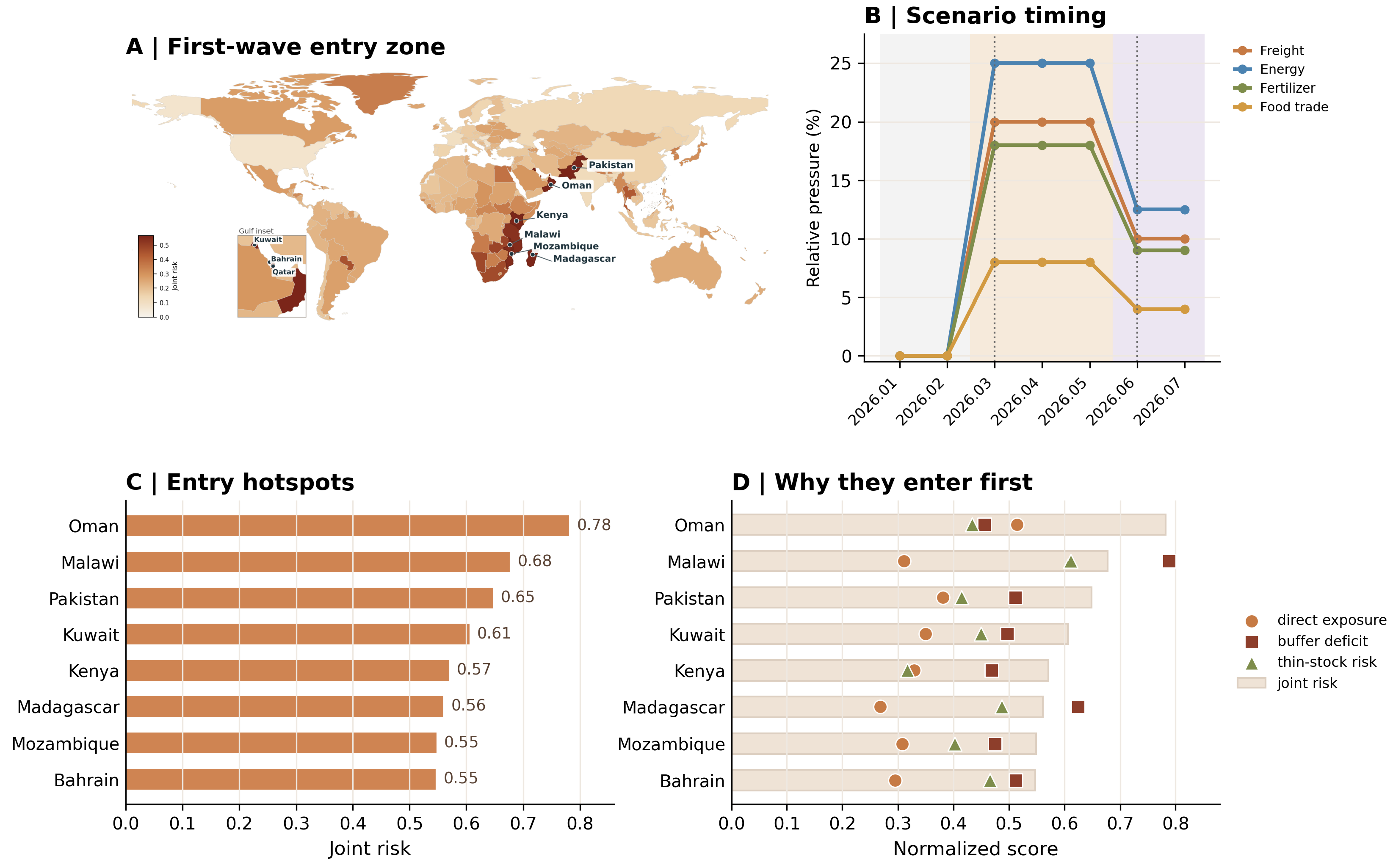
The baseline Hormuz stress test begins with an entry diagnosis rather than a crisis prediction. The hypothetical scenario is inactive in January and February 2026, becomes a full-blockade shock from March to May 2026, and relaxes to limited passage in June and July 2026. During the full-blockade phase, freight spillover is set at 20%, energy price pressure at 25% and fertilizer price pressure at 18%. These are reduced by half in the limited-passage phase. The timing structure shifts the question from general fragility to first contact. It asks which country systems are reached first when a corridor shock is activated and then partially relaxed.

Panel A of Figure 1 shows that the first-wave entry zone is geographically broad. Some high-intensity countries are close to the Gulf, but many are not. The hotspot set includes Oman, Malawi, Pakistan, Kuwait, Kenya, Madagascar, Mozambique and Bahrain, with joint-risk values of about 0.55–0.78. Oman ranks first because its direct exposure is high and its buffer deficit is non-negligible. Malawi ranks second for a different reason. Direct exposure is lower than Oman’s, but buffer deficit and stock shortfall are much larger. Madagascar follows the same pattern. Pakistan and Kuwait lie between these extremes, combining moderate-to-high direct exposure with weaker stock or buffer conditions. The ranking reflects more than maritime proximity.

Panels B–D clarify the timing and composition of the hotspot score. Panel B shows that the entry shock is not a static exposure label. Route, energy, fertilizer and food trade pressures activate during the full-blockade months and then relax during the limited-passage phase. Panels C and D show that the countries at the top of the entry ranking do not all enter for the same reason. Oman is driven mainly by direct exposure. Malawi is driven by buffer deficit and thin-stock risk. Pakistan, Kuwait, Bahrain and Mozambique have a mixed profile. The first-wave set is a joint exposure–buffer ranking rather than a proximity list or a single-variable vulnerability screen.

At this stage, the diagnostic task separates entry from severity. A route-only screen would prioritize countries by affected trade lanes or affected import volumes. A vulnerability-only screen would prioritize countries by general food insecurity or low reserves. The joint entry operator combines both and captures countries that would be missed by either one alone. In the nested entry check, adding buffer deficit to direct exposure improves entry discrimination from an AUC of 0.665 to 0.795 and lowers the Brier score from 0.202 to 0.174. The improvement shows that the first breakpoint is already a coupled systems state, in which physical exposure must interact with weak absorption capacity.

The entry map is not a final food security risk map and should not be used as one. A country can be in the first-wave entry zone and later absorb the shock through inventories, alternative suppliers, public reserves, procurement credit or household support. Conversely, a country outside the top entry list can deteriorate later if it is displaced during market reallocation or if domestic access pressure becomes binding. Its meaning is temporal as well as spatial. It identifies where the shock first arrives, while later state transitions are evaluated in the subsequent layers of the chain.

4.2. Reallocation Pressure Dominates the Modeled Import Availability Response

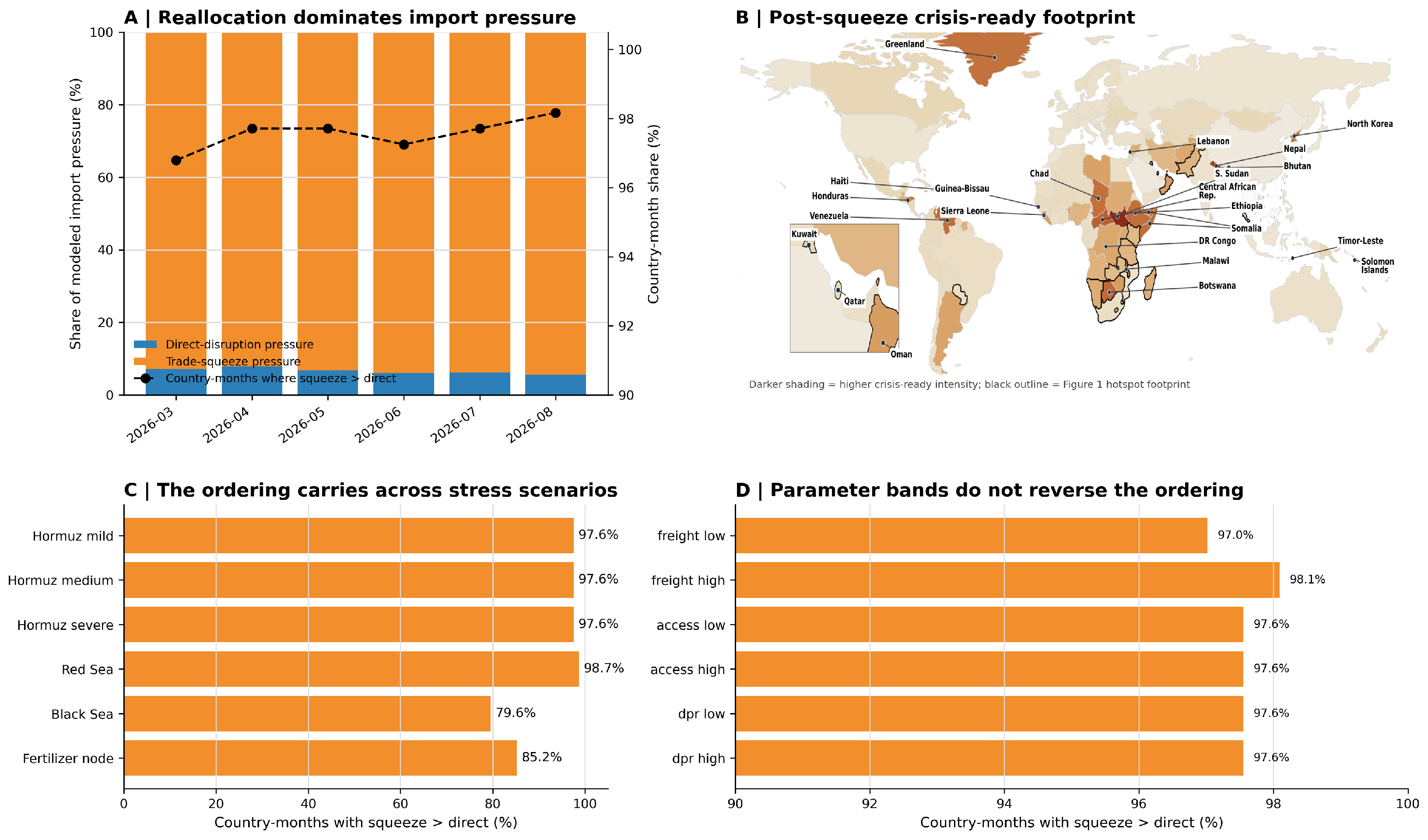
After the entry shock changes route capacity and landed costs, most of the modeled import availability response occurs through the reallocation pressure term rather than the direct corridor term. Panel A of Figure 2 decomposes the normalized pressure index into direct disruption and trade squeeze. The country-mean total pressure is 0.0060, 0.0060, 0.0076, 0.0053, 0.0035 and 0.0023 from March to August 2026. These absolute index values are small because they are averages over all modeled countries, including weakly exposed systems, and they are not tonnes, calories or monetary losses. Within the same monthly totals, trade squeeze accounts for 92.9%, 92.1%, 93.2%, 93.9%, 93.8% and 94.5%, respectively. Direct disruption accounts for the remaining 5.5–7.9%. The share of country–months in which squeeze pressure exceeds direct pressure ranges from 96.8% to 98.2%.

The decomposition does not diminish the role of the strait. Direct disruption activates the stress test and enters both pressure components. The result instead shows that the reduced-form reallocation operator amplifies and redistributes the initial shock through import dependence, energy dependence, supplier concentration and limited logistics support. Countries with similar corridor exposure can therefore receive different total pressures. The squeeze component $S_{i,g,t}$ represents this modeled amplification, while $D_{i,g,t}$ represents the component directly associated with corridor exposure.

Panel B shows the post-squeeze high-pressure footprint. The highlighted countries are not identical to the Figure 1 entry hotspots. Black outlines identify the first-wave hotspot footprint, while darker shading identifies countries with higher total import availability pressure after the squeeze operator is applied. The initial shock is geographically concentrated, but the modeled response spreads through heterogeneous import dependence, supplier concentration, energy exposure, logistics support and domestic absorption capacity. The Gulf inset applies the same comparison to countries close to the corridor. Proximity remains visible, but it does not determine the final pressure ranking.

Panels C and D test whether the ordering is specific to one scenario or parameter setting. Squeeze pressure exceeds direct pressure in 97.6% of country–months under the mild, medium and severe Hormuz variants, 98.7% under the Red Sea case, 79.6% under the Black Sea case and 85.2% under the fertilizer node case. The lower Black Sea and fertilizer node values reflect their different entry mechanisms. The Black Sea event combines conflict and commodity-specific export disruption, while the fertilizer node case enters mainly through agricultural inputs. Neither is a simple substitute for Hormuz. The reallocation strength sensitivity also preserves the baseline ordering. When ${\mu }_S$ is reduced to 0.8, the monthly squeeze share is 90.3–93.2%. When ${\mu }_S$ is raised to 1.2, it is 93.3–95.4%, compared with 92.1–94.5% under the central value.

The mechanism scoreboard clarifies the explanatory roles. If the market reallocation channel is suppressed, squeeze disappears by construction and peak model-Crisis load falls from the baseline mechanism set. If the domestic access channel is suppressed, squeeze still dominates direct loss, but the alert-to-crisis conversion rate falls. Trade squeeze alone is not treated as sufficient for a food security crisis. The two channels play different roles. Squeeze redistributes import pressure, while domestic access turns redistributed import pressure into a food security state transition. A route-only model cannot make this distinction, and a single composite vulnerability index would hide it.

The 92.1–94.5% range is an attribution within the normalized pressure model, not an observed global market share. It should not be generalized to all food crises or read as evidence that physical disruption is trivial. Under the specified Hormuz stress test, direct disruption initiates the response, while the larger modeled component arises from the reallocation pressure operator.

4.3. The Warning-to-Crisis Transition Is a Second-Stage Screening Process

Broad warning does not mechanically lead to a crisis crossing. In the formal baseline country-level alert-to-crisis diagnostic, 161 countries enter model-Alert at least once, but only 39 later cross into model-Crisis or a higher internal model state. The remaining 122 are absorbed or do not worsen further. This split matters because exposed countries are not mechanically escalated. model-Alert means that the external shock has entered the country system. model-Crisis means that the shock has also passed through stock, price, household access and delayed-production layers strongly enough to cross a stricter state threshold.

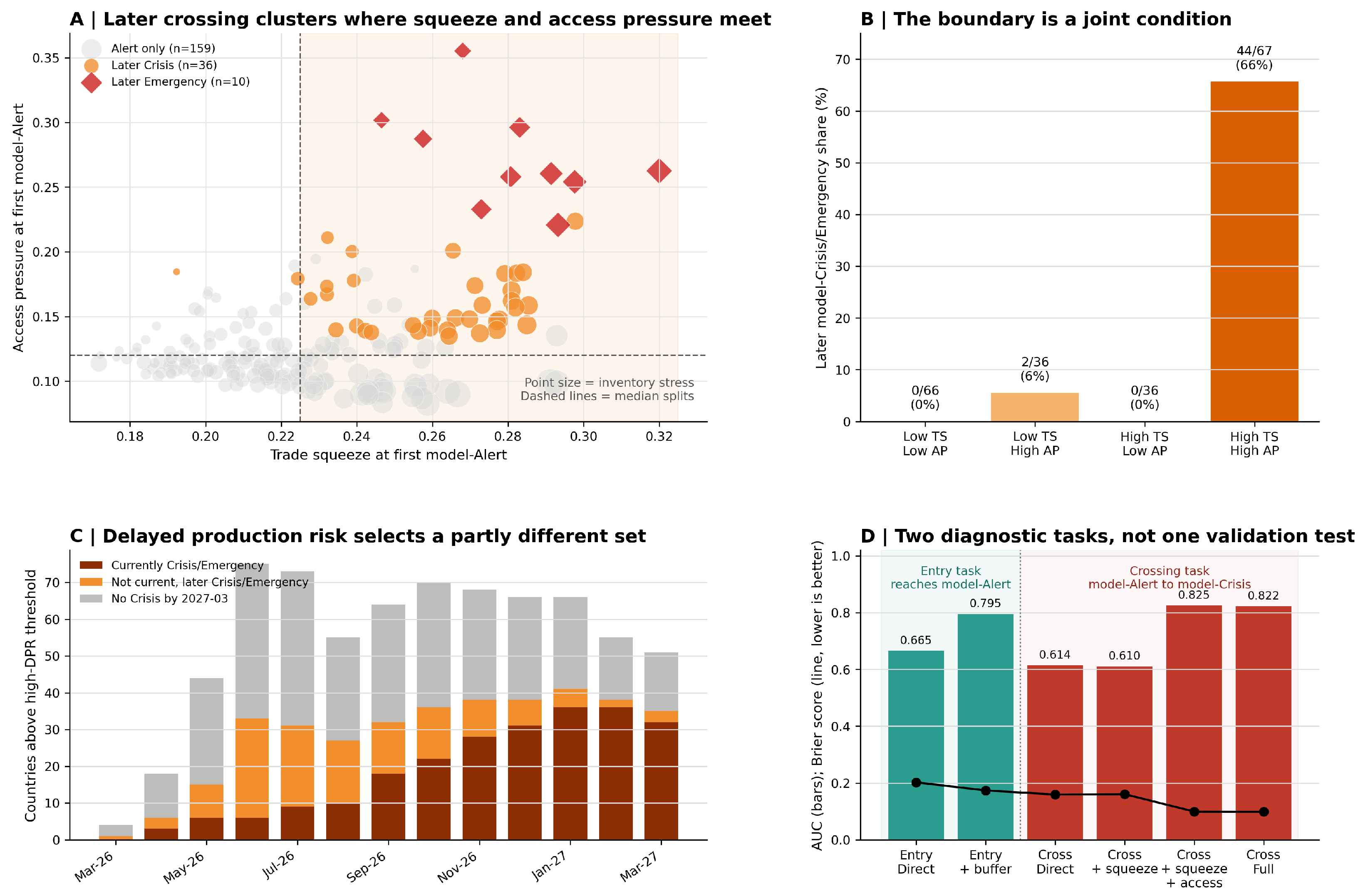
Panel A of Figure 3 visualizes this second-stage screen at the first model-Alert point. The x-axis is trade squeeze, the y-axis is access pressure, and point size indicates inventory stress. Countries that later become model-Crisis or model-Emergency cluster in the upper-right region, where squeeze and access pressure are both high. The lower-right region contains countries with high squeeze but low access pressure, and these do not convert in the quadrant diagnostic. Import displacement is not sufficient by itself. The upper-left region shows the complementary case. High access pressure without high squeeze produces only limited conversion. The boundary is a joint condition, not a one-variable threshold.

Panel B gives the same pattern as a conversion table, but with a different denominator from the formal 161-country baseline diagnostic. The quadrant table uses 205 first-alert records and classifies later model-Crisis or model-Emergency crossing, so the $2+44$ conversions in this panel should be read as a first-alert screening diagnostic rather than as a replacement for the 39-country baseline count. Low squeeze and low access pressure produce no later model-Crisis or model-Emergency cases in the quadrant diagnostic. High squeeze and low access pressure also produce no conversion. Low squeeze and high access pressure produce two conversions out of 36 first-alert records, about 6%. High squeeze and high access pressure produce 44 conversions out of 67 first-alert records, about 66%. Broad model-Alert is not enough. A country needs exposure to market displacement and a domestic access condition that allows the displacement to translate into household pressure.

The formal absorbed-versus-crossing table supports the same interpretation. Mean trade squeeze at first alert is high in both absorbed and crossing pathways, which is why squeeze alone is not enough to separate them. The larger differences appear in access pressure and delayed production risk. Mean access pressure rises from about 0.0145 in absorbed cases to about 0.0166 in crossing cases, and mean delayed production risk rises from about 0.0052 to about 0.0081. These are not large numbers in absolute terms, but they operate at the margin of state thresholds. Their role is to explain why similarly squeezed importers can follow different state paths.

Panel C extends the screen into the production calendar. The high-$DPR$ count rises after the first shock months and peaks before all current crisis states are visible. In March 2026, only four countries exceed the high-$DPR$ threshold. By June and July, the high-$DPR$ set expands to more than 70 countries, with a large group not yet in current model-Crisis or model-Emergency. By late 2026 and early 2027, the currently crisis or emergency component becomes a larger share of the high-$DPR$ stack. This temporal pattern shows why the model separates current access pressure from delayed production risk. A country can look absorbed in the immediate food access layer while still carrying production risk into a later planting or harvest window.

Panel D evaluates the diagnostic gain more directly. For the entry task, direct exposure gives an AUC of 0.665, while direct exposure plus buffer deficit gives 0.795. For the crossing task, direct exposure gives an AUC of 0.614, adding squeeze alone remains weak at 0.610, but adding access pressure raises the AUC to 0.825 and lowers the Brier score from about 0.159 to about 0.099. The full specification remains close to this level, at an AUC of 0.822. The comparison separates two tasks. Entry improves when buffer deficit is added to direct exposure, whereas crossing improves only when access pressure is added to squeeze. A single route exposure score cannot perform both tasks.

The outcome-blinded crossing check addresses circular interpretation. Here, the alternative crossing outcome is built only from direct food disruption, food exposure, baseline vulnerability and baseline household stress. It excludes trade squeeze, access pressure, delayed production risk, crisis-score components and model-state flags. Among 807 first-blind-alert observations, 382 show strict future blind crossing. The entry-only specification gives an in-sample AUC of 0.896 and a Brier score of 0.130. Adding trade squeeze, access pressure, delayed production risk and the squeeze–access interaction raises in-sample AUC to 0.914 and lowers the Brier score to 0.117, while the leave-scenario-out AUC remains similar at about 0.895–0.898. This is a robustness diagnostic rather than an independent causal validation exercise, but the mechanism variables retain the expected sign and discrimination when the outcome is defined without model-state labels.

The state labels should be read within this bounded design. They are internal screening states rather than operational humanitarian categories. They measure state transitions inside a controlled pressure test. The transitions show why some alerts are absorbed, why some become crisis, and why some carry delayed production risk before current access conditions deteriorate.

4.4. Observed Disruption Windows Are Consistent with the Screening Direction

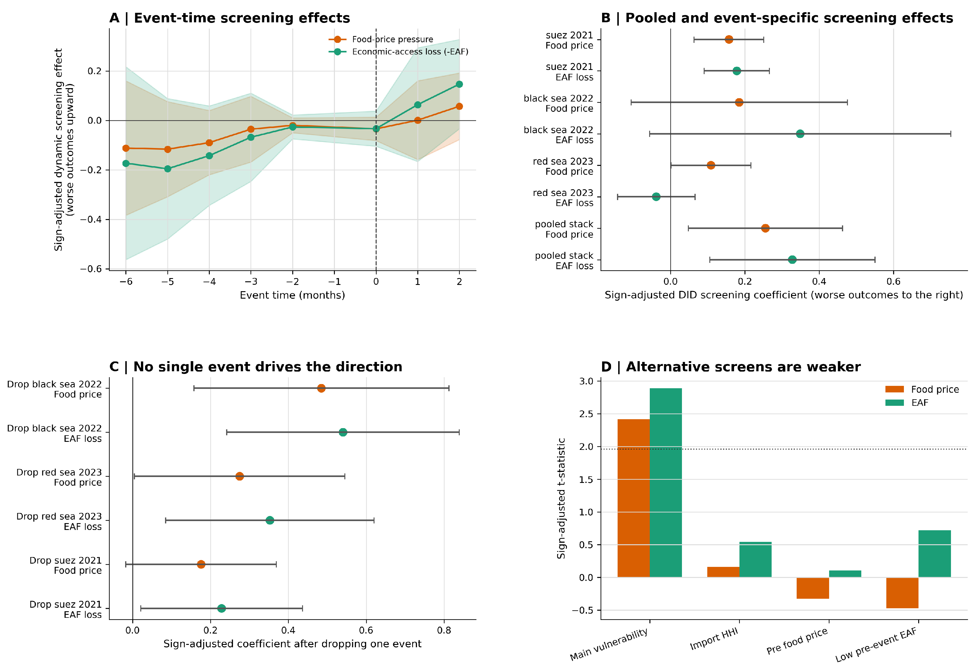
The modeled exposure–vulnerability interaction is compared with three observed disruption windows. These are the 2021 Suez blockage, the 2022 Black Sea shock and the 2023 Red Sea shock. Figure 4 uses these events to test a narrower proposition, not to reconstruct every model operator. After observed disruptions, countries that are both exposed and vulnerable should show stronger food price pressure or economic access deterioration than countries without that exposure–vulnerability combination.

Panel A reports sign-adjusted event-time coefficients, where positive values indicate worse outcomes in the expected direction. The pre-event diagnostic is not uniform across events. Relative to month $-1$, four of the five Suez coefficient estimates for months $-6$ to $-2$ have absolute t-statistics above 1.96 for both food price pressure and the economic access factor. None of the corresponding Black Sea or Red Sea coefficient estimates meet that criterion. The Suez comparison therefore fails a strict parallel trends screen. Post-event movement in the expected direction is reported as descriptive evidence of exposure–vulnerability association, not as a causal effect of the disruption.

Panel B shows pooled and event-specific estimates. In the three-event pooled post-window model, the food price coefficient is 0.255 with a standard error of 0.106 and a t-statistic of 2.42. The economic access coefficient is −0.328 with a standard error of 0.113 and a t-statistic of −2.89. The stacked specification uses 37,932 observations, 218 country clusters and 654 event–country fixed effects. These estimates summarize conditional post-event differences in the stacked sample. Because the Suez pretrend is non-flat and the events are not exchangeable, the coefficients are not interpreted as causal validation of the Hormuz model.

The event-specific estimates reveal heterogeneity. The Suez window has the clearest two-outcome pattern, with positive food price pressure and adverse economic access movement. The Black Sea window has the expected signs for both outcomes, but confidence intervals are wider, consistent with a broader geopolitical and commodity-specific shock. The Red Sea window preserves the expected sign for food price pressure, while the economic access estimate is not adverse in the same way. These mixed results support only a narrower interpretation. The pooled and most event-specific estimates point in the same screening direction, while individual events differ in duration, commodity scope and transmission channel.

Panel C reports leave-one-event-out estimates. Dropping the Black Sea, Red Sea or Suez event preserves a positive food price coefficient and a negative economic access coefficient, although magnitudes change. This sign stability reduces dependence on one episode but does not repair event-specific identification limitations. It supports only the narrower claim that exposure combined with vulnerability is a recurring screening signal across the selected windows.

Panel D compares the main vulnerability screen with simpler alternatives. The main pre-event severe food insecurity screen gives sign-adjusted t-statistics of 2.42 for food price pressure and 2.89 for economic access deterioration. Alternative screens based on import concentration, pre-event food price level or low pre-event economic access fraction are weaker in the stacked design. The comparison shows that the selected vulnerability screen aligns more closely with both outcomes than these simpler alternatives.

The historical evidence remains deliberately bounded. It does not causally identify all channels in the scenario model, including private trader allocation, political bargaining, contract enforcement, sanctions, naval risk pricing, humanitarian distribution or informal trade. Its role is to provide a bounded external check on the direction of the screening logic. The scenario model resolves the represented mechanisms, whereas the historical panel assesses their plausibility against observed events. The two forms of evidence answer different questions and are interpreted as complementary rather than interchangeable.

4.5. Policy Value Is Breakpoint-Specific and Time-Sensitive

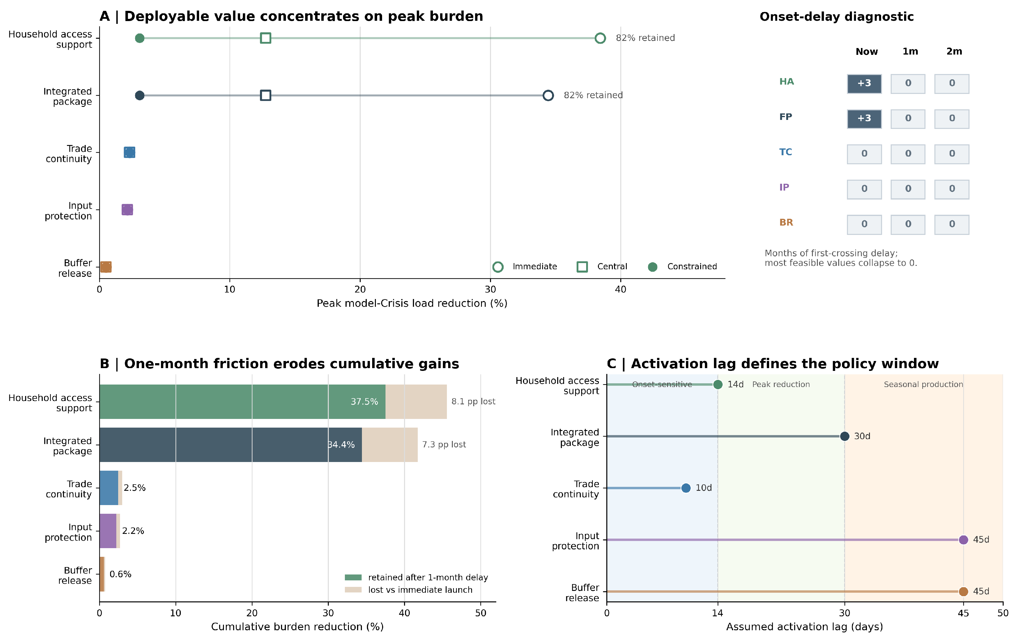
The policy experiment is diagnostic rather than a ranking table. Figure 5 compares household access support, an integrated package, trade continuity, input protection and buffer release. The integrated package combines buffer release, import diversion, household subsidy, demand management and logistics support. At the central policy intensity, their normalized perturbations are 0.64, 0.60, 0.68, 0.28 and 0.68, respectively. These are standardized model inputs, not equal-cost real fiscal packages. The comparison identifies the binding breakpoint in the baseline stress test and measures how much intervention value survives deployment delay.

Panel A shows deployable peak load value. Under immediate deployment, household access support reduces peak model-Crisis load by 38.4%, the peak population count in model-Crisis-or-higher states by 67.9% and cumulative model-state burden by 45.6%. The integrated package reduces peak load by 34.4% and cumulative model-state burden by 41.7%. Trade continuity, input protection and buffer release generate much smaller peak load reductions under the reported metric. The smaller peak-load effects do not imply that upstream instruments lack value. By the time peak model-Crisis load is measured, the active binding layer in the baseline stress test is domestic access rather than only route capacity, delayed production or stock release.

The onset delay diagnostic gives a different answer. With immediate deployment, household access support and the integrated package delay first crossing by three months. With a one-month delay, the onset delay gain collapses to zero. These metrics measure different timing margins. Onset delay is a threshold-timing outcome. It can be achieved only if intervention reaches the system before the relevant state transition. Once the transition has occurred, a later intervention can reduce burden but cannot retroactively delay the first crossing. The timing metric is separated from peak reduction and cumulative burden.

Panel B shows the burden effect after one-month friction. Household access support still reduces cumulative burden by 37.5%, losing about 8.1 percentage points relative to immediate deployment and retaining 82.3% of its immediate burden reduction value. The integrated package reduces cumulative burden by 34.4%, losing about 7.3 percentage points and retaining 82.5% of its immediate value. By contrast, peak load reduction falls much more sharply. Household access support falls from 38.4% to 12.8%, and the integrated package falls from 34.4% to 12.8%. With a two-month delay, peak load gains fall to about 3.1%, while burden reduction remains 28.5% for household access support and 26.3% for the integrated package. The policy implication is not just “act early”. Different policy metrics decay at different rates.

Panel C connects these values to operational lags. Household access support is represented as onset-sensitive and fast, around 14 days. Trade continuity is also fast, around 10 days, but it acts upstream on the squeeze process. The integrated package is slower, at around 30 days, and input protection and buffer release are represented with longer activation lags, at around 45 days. Placing these instruments on the same propagation timeline shows why a slower instrument can still be valuable for a delayed production or stock breakpoint but may fail to delay first crisis crossing if that crossing occurs before implementation.

Immediate deployment identifies the binding layer, with access support and the integrated package producing the largest peak and cumulative burden reductions under baseline timing. Deployment friction then separates fragile onset-delay gains from more persistent cumulative-burden gains. The activation-lag comparison further shows that a package’s practical value depends on reaching the relevant breakpoint in time as well as on its theoretical target. Together, these results turn policy comparison from a static ranking into a threshold-specific deployment problem.

The estimates should not be read as a cost-effectiveness ranking. The modeled interventions are not equal-cost programs and do not include targeting error, fiscal constraints, political feasibility, procurement bottlenecks or administrative leakage. The results instead concern the active breakpoint. If the crisis chain has already moved into household access, route-only measures are unlikely to dominate the measured model-Crisis outcome. If the chain is still upstream, access support may protect households but may not preserve market position. If the main threat is delayed production, input protection can be valuable even when current peak model-Crisis load effects are modest. The practical rule is to match the instrument to the active breakpoint and deploy it before the relevant threshold closes.

5. Discussion

5.1. Findings and Mechanism Interpretation

The Hormuz stress test separates first contact with the trade system from subsequent state deterioration. Countries near the corridor can enter through high direct exposure, as in the case of Oman, while geographically distant countries can enter because limited stocks and weak buffers leave little capacity to absorb a smaller external shock. The first-wave map is therefore a joint exposure–absorption screen. It should not be interpreted as a ranking of final food security outcomes.

Most modeled import availability pressure is assigned to the reallocation component after the corridor shock is introduced. Country-mean total pressure ranges from 0.0023 to 0.0076 during March–August 2026, and trade squeeze contributes 92.1–94.5% of that normalized quantity. Varying the reallocation strength multiplier by $\pm 20\%$ changes the corresponding range to 90.3–93.2% and 93.3–95.4%, without reversing the ordering. This result is conditional on the reduced-form pressure specification. It indicates that the modeled burden is amplified by import dependence, energy dependence, supplier concentration and limited logistics support. It is not an estimate of displaced tonnage or an observed global allocation share.

The distinction between entry and crossing explains why a broad shock footprint does not produce uniform escalation. Among the 161 countries that enter model-Alert, 39 later reach model-Crisis or a higher internal state. In the separate 205-record quadrant diagnostic, high squeeze without high access pressure produces no later conversion, whereas 44 of 67 records with both high squeeze and high access pressure convert. The counts use different units of observation, but both diagnostics point to the same mechanism. Reallocation pressure changes import availability, while domestic access and delayed production conditions determine whether that pressure crosses a more severe threshold.

The historical panel provides a limited external consistency check rather than causal or predictive validation. No Black Sea or Red Sea pre-event coefficient estimate exceeds the reported threshold, but four of the five Suez pre-event coefficient estimates have absolute t-statistics above 1.96 for both outcomes. The pooled post-event associations and leave-one-event-out signs remain informative as directional evidence, yet the non-flat Suez pretrend prevents a difference-in-differences causal interpretation. The manuscript therefore presents a screening framework supported by scenario case studies and limited historical comparison, not a fully validated predictive model. Policy experiments provide a separate within-model result. Household support and the integrated package reduce peak and cumulative burden when deployed immediately, while their ability to delay the first crossing disappears after a one-month implementation delay.

5.2. Relation to Established Modeling Approaches

Table 1 places the framework against representative system dynamics, bullwhip, interdependent network, food production network and chokepoint models. The framework draws on these established ideas rather than claiming new underlying supply chain phenomena. Stocks, delays and state transitions follow system dynamics logic, but the unit is a country–commodity–month pressure rather than an aggregate stock. Amplification is related to bullwhip reasoning, but the outcome is cross-country food access stress rather than upstream order variance. Interdependent and multilayer networks motivate propagation across connected units, while the present decomposition adds maritime entry, importer-level reallocation, household access and crop calendar timing in a common state-crossing screen. Its methodological contribution is this ordered decomposition and the separation of entry, crossing and intervention tasks.

This distinction also bounds the meaning of resilience. The reported model tests absorption, survivability and recovery within a fixed network. Scenario inputs can degrade existing route and supplier edges, but the solver does not create new routes, modes, suppliers or contracts. Adaptability and transformability require endogenous reconfiguration and are not measured here. The terms entry, crossing and breakpoint refer only to the timing of model-state transitions and intervention opportunities.

Hormuz is the focal case, not a generic empirical representation of all chokepoints. Its modeled shock couples freight, energy, fertilizer and food trade channels. Suez was a short physical blockage, the Black Sea shock combined conflict, sanctions and commodity-specific export disruption, and the Red Sea episode mainly altered routing, risk premia and transit time. The related scenarios test whether the ordering of model components survives different entry assumptions. They do not establish equal magnitudes, common causal structures or universal validity across maritime disruptions.

The state labels are similarly restricted. model-Alert, model-Crisis and model-Emergency are internal thresholds of a normalized screening index. They are not IPC, FEWS NET, WFP or famine classifications, and they cannot replace field assessments or household surveys. Their purpose is to make the transition logic auditable under a controlled stress test.

5.3. Managerial and Policy Implications

Operational monitoring should distinguish the layer at which pressure is accumulating. Route exposure and freight changes identify entry. Import dependence, supplier concentration, energy exposure and logistics capacity indicate whether the initial shock is being amplified. Food prices, affordability and social protection capacity indicate whether import pressure is reaching households. Fertilizer and energy exposure combined with crop calendars indicate whether a later production constraint is developing. A dashboard that reports only affected routes or tonnage can miss these transitions.

Intervention choice should follow the same sequence. Trade continuity and import diversion act before reallocation pressure is fully transmitted. Buffer release and household support act on domestic absorption and access. Input protection targets delayed production risk. The integrated package combines all five modeled instruments, but its slower deployment means that it can retain cumulative burden value after losing the opportunity to delay the first crossing. The practical comparison is therefore breakpoint-specific and time-dependent, not a cost-effectiveness ranking among real programs.

5.4. Limitations and Future Work

The reallocation component is a reduced-form pressure operator. It does not clear a physical market and does not observe firm-level contracts, bids, credit lines, elasticities, shipment capacities or procurement priorities. Softmax, CES, auction and linear programming alternatives would require behavioral or market-clearing assumptions that the available cross-country data cannot identify. A gravity specification could characterize bilateral trade propensity, but it would not by itself allocate scarce short-run supply across importers. The formulation therefore varies the implemented reallocation strength directly and reports the resulting sensitivity. The 92.1–94.5% central share must be read as a property of that stress test specification, not as a measured property of the global food system.

Fixed topology is a second limitation. Actual crisis response may create new suppliers, routes and transport modes. Future work could replace the exogenous trade continuity perturbation with a multi-objective flow problem that balances delivery time, cost, reliability and food security priority under route, terminal and mode constraints. Decomposition-based multimodal path optimization provides one possible computational approach, but it requires route-level capacities and operational data that are unavailable in the present study.

Monthly aggregation is appropriate for the common resolution of trade, price and food security inputs, but it can conceal within-month tipping points. Two disruptions occurring at different dates in the same month may receive the same scenario value, and a two-week delay in fertilizer delivery can matter even when the monthly average appears moderate. Delayed production results should therefore be interpreted as vulnerable planting or harvest months, not exact weekly deadlines.

The historical design has its own limits. The event windows are heterogeneous, the Suez pretrend is non-flat, and the pooled specification cannot isolate private allocation, sanctions, political bargaining, insurance pricing, informal trade or humanitarian distribution. The event panel is retained as a directional comparison only and does not validate the full operator sequence, threshold partition or predictive accuracy of the model. More credible validation would require event-specific controls, higher-frequency observed outcomes, pre-registered exposure definitions, stronger counterfactual designs and out-of-sample assessment across held-out disruptions.

Finally, country–commodity aggregation compresses local heterogeneity. Route-level AIS data, freight and insurance premia, trade-finance records, supplier contracts, reserve releases, weekly crop calendar data and household welfare observations would allow direct estimation of operators that are currently specified heuristically. Such data would also support endogenous network reconfiguration, out-of-sample validation and policy simulations expressed in physical or monetary units.

6. Conclusions

This study develops a monthly resilience screening model for a hypothetical Strait of Hormuz closure. The model separates direct disruption, reallocation pressure, household access and delayed production risk within a fixed global food trade structure. It is designed to locate transitions in a stress test sequence rather than forecast an actual closure or assign humanitarian classifications.

In the baseline scenario, country-mean import availability pressure ranges from 0.0023 to 0.0076 during March–August 2026. Trade squeeze accounts for 92.1–94.5% of that normalized pressure, and the ordering remains under a $\pm 20\%$ change in reallocation strength. Of the 161 countries entering model-Alert, 39 later reach model-Crisis or a higher internal state. Escalation concentrates where reallocation pressure coincides with weak household access and delayed production risk. These findings are conditional on the stated scenario, parameters and reduced-form operators.

The historical windows provide only a limited external consistency check because the events differ and the Suez pretrend is non-flat. They do not establish predictive validation. Intervention experiments show that modeled policy value depends on both the active layer and deployment timing. The resulting contribution is a case-study-supported systems diagnostic for identifying whether pressure is concentrated at route entry, import reallocation, household access or the production calendar, and for determining which modeled intervention window remains open.