Article

Supply Chain Shocks and the Reconfiguration of Green Finance Markets: A Quantile-on-Quantile Connectedness Analysis


1
School of Economics and Management, University of Chinese Academy of Sciences, Beijing 100190, China
2
Beijing Key Laboratory of Topological Statistics and Applications for Complex Systems, Beijing Institute of Mathematical Sciences and Applications, Beijing 101408, China
3
Digital Economy Laboratory, Beijing Institute of Mathematical Sciences and Applications, Beijing 101408, China
4
PBC School of Finance, Tsinghua University, Beijing 100084, China
5
Research Institute of The People’s Bank of China, Beijing 100033, China
*
Author to whom correspondence should be addressed.
Systems 2026, 14(6), 652; https://doi.org/10.3390/systems14060652
Submission received: 20 April 2026 / Revised: 3 June 2026 / Accepted: 4 June 2026 / Published: 6 June 2026

Abstract

Supply chain disruptions have become a major source of macro-financial stress, yet their implications for green finance remain underexplored. This paper investigates the state-dependent connectedness between supply-side bottlenecks and the green finance market, represented by clean energy equities, green bonds, and carbon prices. Using daily data on regional Supply Bottleneck Indices (SBIs) for China, the United States, and the euro area, we first construct a global Supply Bottleneck Index (GSBI) by principal component analysis and then estimate pairwise quantile-on-quantile connectedness (QQC) between supply bottleneck indicators and each green finance submarket. The results show that connectedness is strongly nonlinear, asymmetric, and time-varying. For the global indicator, connectedness intensifies at both joint and cross-tail quantile combinations, while mid-quantile states exhibit weak coupling. Regional results reveal clear heterogeneity: China and the United States display the strongest connectedness with clean energy equities in extreme upper-tail states, whereas the euro-area indicator is most tightly linked with the carbon market. Across many extreme states, supply bottleneck indicators show positive net connectedness with green finance markets, but green finance markets, especially carbon prices, can dominate the bilateral connectedness relation under calmer or intermediate regimes. Robustness checks based on average and quantile-rank GSBI constructions, a post-2023 subsample, and alternative QQC tuning choices support the tail-dominance pattern. These findings suggest that supply bottlenecks are not uniformly related to all green assets; rather, they are associated with state-dependent changes in the internal connectedness architecture of the green finance system. The paper contributes to the literature on financial connectedness and sustainable finance by showing how a real-economy disturbance is associated with changes in the connectedness and resilience of green financial markets.

1. Introduction

Real supply-side disruptions have become a defining feature of the post-pandemic macro-financial environment. Episodes such as the COVID-19 pandemic [1], the semiconductor shortage [2], the Suez Canal blockage [3], and the Russia–Ukraine war [4] have disrupted production networks, transport routes, and trade flows, thereby intensifying inflationary pressures, tightening financial conditions, and raising macroeconomic uncertainty [5,6,7,8]. These shocks have also highlighted the fragility of globally integrated supply chains and increased the demand for timely indicators capable of capturing production bottlenecks, delivery delays, and logistics frictions as they arise [9,10,11]. In this respect, the text-based Supply Bottleneck Index (SBI) proposed by Burriel et al. [12] offers a particularly useful high-frequency measure of real-economy supply stress.
At the same time, green finance has emerged as a central segment of modern financial markets [13]. It plays a dual role: it channels capital toward decarbonization and climate-aligned investment, and it provides a market-based mechanism for pricing transition-related risks [14,15]. This role is also grounded in sustainable asset-pricing theory: investor preferences for sustainability and climate-related risks can affect expected returns, valuation ratios, and portfolio demand for green assets [16]. Yet green finance is not a single asset class. Rather, it is a multi-segment system comprising clean energy equities, green bonds, and carbon markets, which respectively reflect the valuation, financing, and regulatory-pricing dimensions of the sustainability transition [17,18,19,20,21,22,23]. The increasing importance of these markets implies that external real-economy shocks, including supply bottlenecks, may have consequences not only for industrial activity and inflation, but also for the internal connectedness structure of green financial markets [24,25,26,27,28].
Existing studies have primarily analyzed these two issues separately. On the one hand, a growing macro-finance literature shows that supply disruptions affect inflation, output volatility, and financial conditions [7,8,10,11,29,30,31]. On the other hand, the green-finance literature has documented substantial connectedness within green assets and between green and conventional markets, especially during periods of market stress [17,18,20,21,24,25,26,27]. However, much less is known about how supply-side disruptions originating outside the financial sector are associated with green-finance connectedness, or whether different green submarkets react heterogeneously to global and regional supply bottlenecks.
Against this backdrop, this paper investigates the connectedness between supply chain bottlenecks and three core green finance markets: clean energy equities (CE), green bonds (GB), and carbon market (Carbon). These three markets are selected because they represent distinct risk profiles and regulatory environments within the green finance ecosystem, allowing us to capture potential heterogeneity in how supply-side stress propagates across segments. On the supply-chain side, we employ the daily newspaper-based Supply Bottleneck Index (SBI) for China, the United States, and the euro area, three economies that collectively dominate global trade flows, and construct the GSBI via principal component analysis (PCA) to extract their common variation [32]. On the green-finance side, clean energy equities, green bonds, and carbon allowances (represented by ICE EUA futures) are chosen to span equity, fixed-income, and derivative dimensions of green finance. Because supply disruptions and financial market dynamics are unlikely to be linear or state-invariant, we adopt the quantile-on-quantile connectedness (QQC) framework of Gabauer and Stenfors [33], which jointly conditions on the quantile states of both variables in each bivariate system. This allows us to evaluate whether the strength, direction, and persistence of connectedness vary across bearish, normal, and bullish market conditions, and whether the regional origin of supply-side stress matters economically.
This paper contributes to the literature in three ways. First, it introduces real-economy supply chain disturbances into the analysis of green finance connectedness and shows that the strongest links appear in joint- and cross-tail states rather than in normal market conditions. Second, it connects the regional origin of bottlenecks to the heterogeneous structure of green finance: clean energy equities are more tightly linked to China and U.S. bottlenecks, whereas carbon prices are especially sensitive to euro-area bottlenecks. Third, it extends the green-finance connectedness literature from within-system interactions to externally associated system reconfiguration, while explicitly treating the estimates as state-dependent dependence rather than structural causal effects.
The remainder of the paper is organized as follows. Section 2 discusses the theoretical linkages and related literature. Section 3 presents the data and methodology. Section 4 reports the empirical findings for global and regional supply chain shocks. Section 5 concludes.

2. Theoretical Linkages Between Supply Chain Disruptions and Green Finance Markets

2.1. Supply Chain Shocks, Economic Mechanisms, and Green Finance Connectedness

Supply chain bottlenecks are external real-economy shocks that alter production costs, delivery schedules, input availability, and transport efficiency [34]. Through these channels, they affect inflation expectations, uncertainty, discount rates, and funding conditions, with implications that extend well beyond trade and industrial production [5,6,7,8,10,11,31]. From an asset-pricing perspective, such shocks can influence both expected cash flows and required returns, implying that the financial consequences of supply disruptions are likely to be nonlinear and state-dependent [29].
These mechanisms are especially relevant for green finance. Clean energy equities are directly exposed to fluctuations in supply-chain conditions because renewable-energy equipment, batteries, semiconductors, and critical inputs are embedded in complex international production networks [35]. Green bonds are linked to the financing of climate-aligned projects, and their risk–return profile may change when supply bottlenecks alter project timelines, refinancing conditions, or investor sentiment [36,37]. Carbon markets are tied to the regulatory price dimension of the transition, and their response to supply disruptions may reflect changes in industrial activity, energy substitution, and compliance expectations [38,39]. Accordingly, supply chain shocks need not affect all green-finance segments in the same manner.
Three mechanisms guide the empirical interpretation. The first is a cash-flow channel: bottlenecks in equipment, batteries, semiconductors, and critical minerals can delay clean-energy deployment and alter expected revenues for transition-related firms. The second is a discount-rate and financing channel: persistent supply stress can raise inflation and interest-rate expectations, thereby affecting green bond valuations and the financing cost of climate-aligned projects. The third is a policy-pricing channel: supply disruptions can change energy substitution incentives, industrial output, and compliance demand, which are directly relevant for carbon allowance prices. These channels imply that regional bottlenecks should not be interchangeable. China is closely tied to clean-energy manufacturing and upstream inputs, the United States is central to technology, financing, and global risk sentiment, and the euro area is institutionally connected to the EU ETS and carbon-pricing regime.
The recent green-finance literature provides several reasons to expect heterogeneous and asymmetric connectedness across these markets. Reboredo [17] show that green bonds co-move more strongly with fixed-income markets than with energy commodities, implying diversification opportunities but also heterogeneous exposure to external shocks. Liu et al. [20] document asymmetric dependence and risk spillovers between green bonds and clean energy markets. Naeem et al. [22] extend this asymmetric perspective to the green bond–commodity nexus, showing that the relationship is concentrated in the tails of the joint distribution and becomes most pronounced under extreme market conditions. Pham [21] show that the strength of the relationship between green bond and green equity markets varies across quantiles and investment horizons. Reboredo and Ugolini [18] and Reboredo et al. [19] further show that green bonds are connected to broader financial markets, but often in a way that preserves diversification value. Related evidence by Hammoudeh et al. [40] emphasizes that the relationship between green bonds and financial or environmental variables is itself time varying. Using green financial portfolios that explicitly include carbon prices, Tiwari et al. [23], Chatziantoniou et al. [25], and Ringstad and Tselika [26] find that spillovers within green finance intensify during turbulent periods and that carbon prices often play a distinct role relative to green bonds and clean energy assets. More recently, Wang et al. [27] and Huang et al. [28] provide evidence that risk spillovers within green financial systems are highly dynamic and subject to structural heterogeneity.

2.2. Research Gap and Positioning of This Paper

By contrast, the literature on supply bottlenecks has focused mainly on macroeconomic and broad financial outcomes rather than on green finance as a system. The SBI of Burriel et al. [12] provides a timely narrative-based measure of supply bottlenecks, while recent studies show that elevated supply pressures can feed into inflation dynamics, output fluctuations, and tighter financial conditions [7,8,10,11,29,30,31]. Yet the existing evidence rarely distinguishes between global and regional sources of supply-side stress, and even more rarely asks how such shocks propagate into different segments of green finance.
This gap is important for two reasons. First, the green finance system is internally heterogeneous: valuation, financing, and regulatory-pricing channels may react differently to the same external disturbance [23,26]. Second, green-finance connectedness is known to strengthen in stressed states, implying that the effect of supply bottlenecks is unlikely to be adequately summarized by mean-based models [25,26]. For this reason, a state-dependent connectedness framework is particularly appropriate.
Our paper is closest in spirit to Youssef et al. [32], who show that supply bottlenecks and cryptocurrency markets are connected in a strongly nonlinear and quantile-dependent manner. We extend this external-shock perspective to a green financial system composed of clean energy equities, green bonds, and carbon prices. Rather than focusing on a single structural channel, we examine whether supply chain shocks reconfigure the internal connectedness structure of green finance, and whether such reconfiguration depends on market states and on the regional origin of supply-side stress. To synthesize the gaps identified above, Table 1 places this paper within the landscape of the most closely related studies by comparing market coverage, methodological choices, and key analytical features. The comparison reveals that existing work has addressed either the internal connectedness of green finance or the macroeconomic consequences of supply bottlenecks, but not the two together within a state-dependent framework that simultaneously covers clean energy equities, green bonds, and carbon markets across both global and regional supply chain indicators.

3. Data and Methodology

3.1. Data

The empirical analysis uses daily data on four supply chain shock indicators and three green finance market indices over the common sample from 2 January 2018 to 31 March 2026. Supply chain bottlenecks are measured using the daily newspaper-based Supply Bottleneck Indices (SBI) provided by Banco de España [12].1 The raw database contains country-level series for the United States, China, and several European economies, together with an aggregate euro-area indicator. We retain the China, United States, and euro-area series as our regional indicators and denote them as S B I C H N , S B I U S A , and S B I E U R , respectively. On the green-finance side, we use the S&P Clean Energy Index to proxy clean energy equities (CE),2 the S&P Dow Jones Green Bond Index to proxy green bonds (GB),3 and the daily settlement price of a continuous ICE EUA futures series under the EU ETS to proxy the carbon market (Carbon).4 The carbon variable uses the provider’s continuous settlement-price series for EUA futures exposure. This series is useful for maintaining a daily carbon-price proxy over a long sample, but it does not allow us to reconstruct contract-level roll dates, roll yields, or alternative maturity-specific EUA futures. We therefore interpret the carbon proxy as a continuous futures-price indicator rather than as a contract-specific return strategy, and we return to this limitation in the conclusion. This market design follows a large part of the green-finance connectedness literature, which treats clean energy, green bonds, and carbon prices as the three core segments of a green financial system [25,26].
The calendar is aligned by retaining dates common to all seven series and dropping observations with missing or nonpositive values before return construction. The aligned level sample contains 2121 observations from 2 January 2018 to 31 March 2026, and the final transformed sample contains 2120 daily observations from 3 January 2018 to 31 March 2026. Regional SBI series are positive newspaper-based stress indices and are transformed into log changes, r i , t = ln ( p i , t ) ln ( p i , t 1 ) . Green finance price series are transformed in the same way. The economic interpretation differs, however. For asset prices, log returns measure financial gains and losses. For the newspaper-based SBI, log changes measure innovations in bottleneck pressure rather than the absolute pressure level. This transformation is appropriate for the connectedness analysis because the QQC framework is applied to stationary daily changes and because green financial markets are expected to react most strongly to news about worsening or easing supply stress. The cost is that very persistent bottleneck levels are represented through repeated daily changes within the rolling window rather than through the raw level itself. We therefore interpret the SBI variables as short-run changes in supply-chain pressure, not as long-run level measures of disruption intensity. The PCA-based GSBI can take positive or negative values because it is a standardized factor score, so it is transformed by first differences rather than log differences. This treatment preserves the interpretation of increases in the global factor as increases in common supply bottleneck pressure while avoiding an invalid logarithmic transformation.
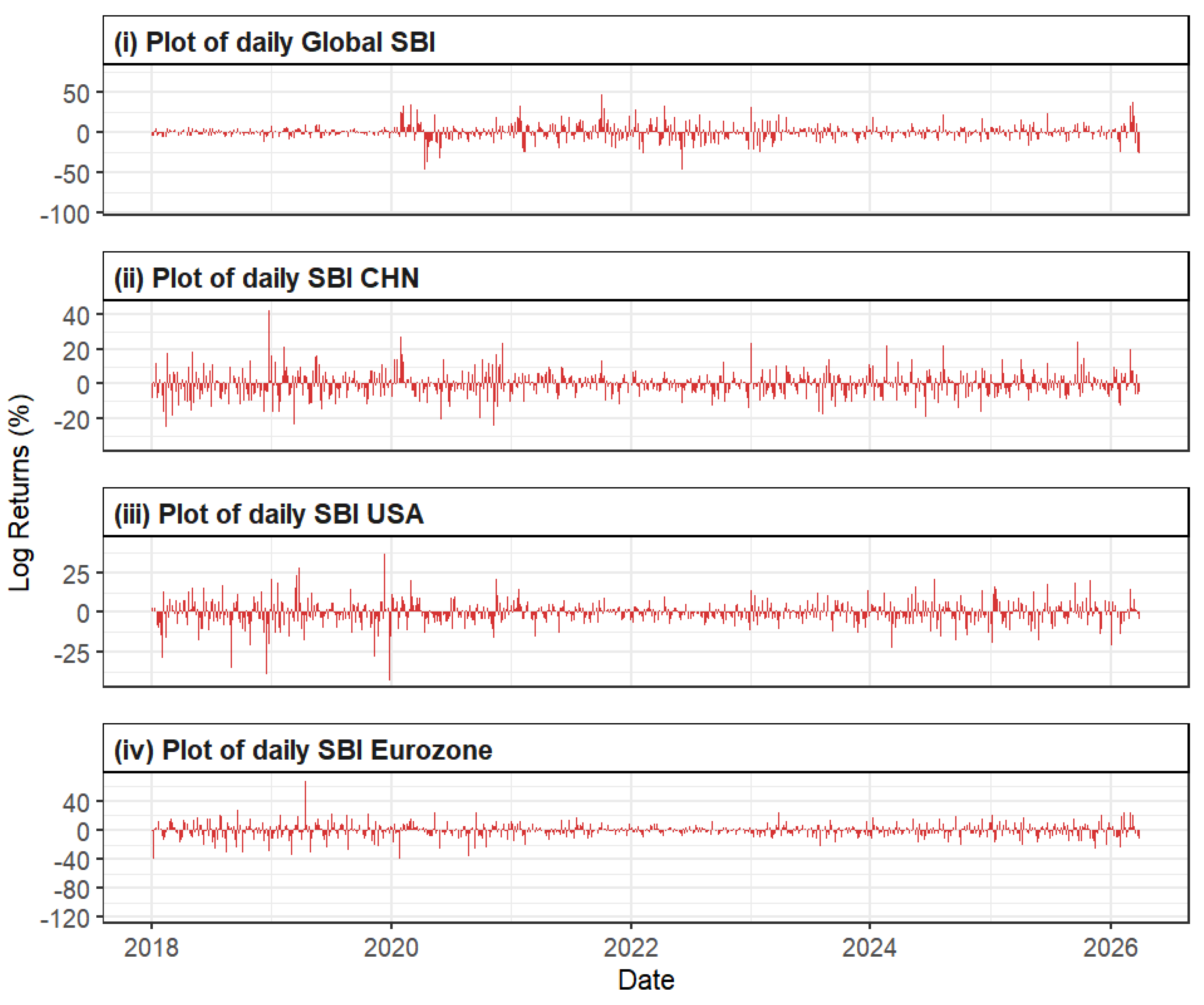
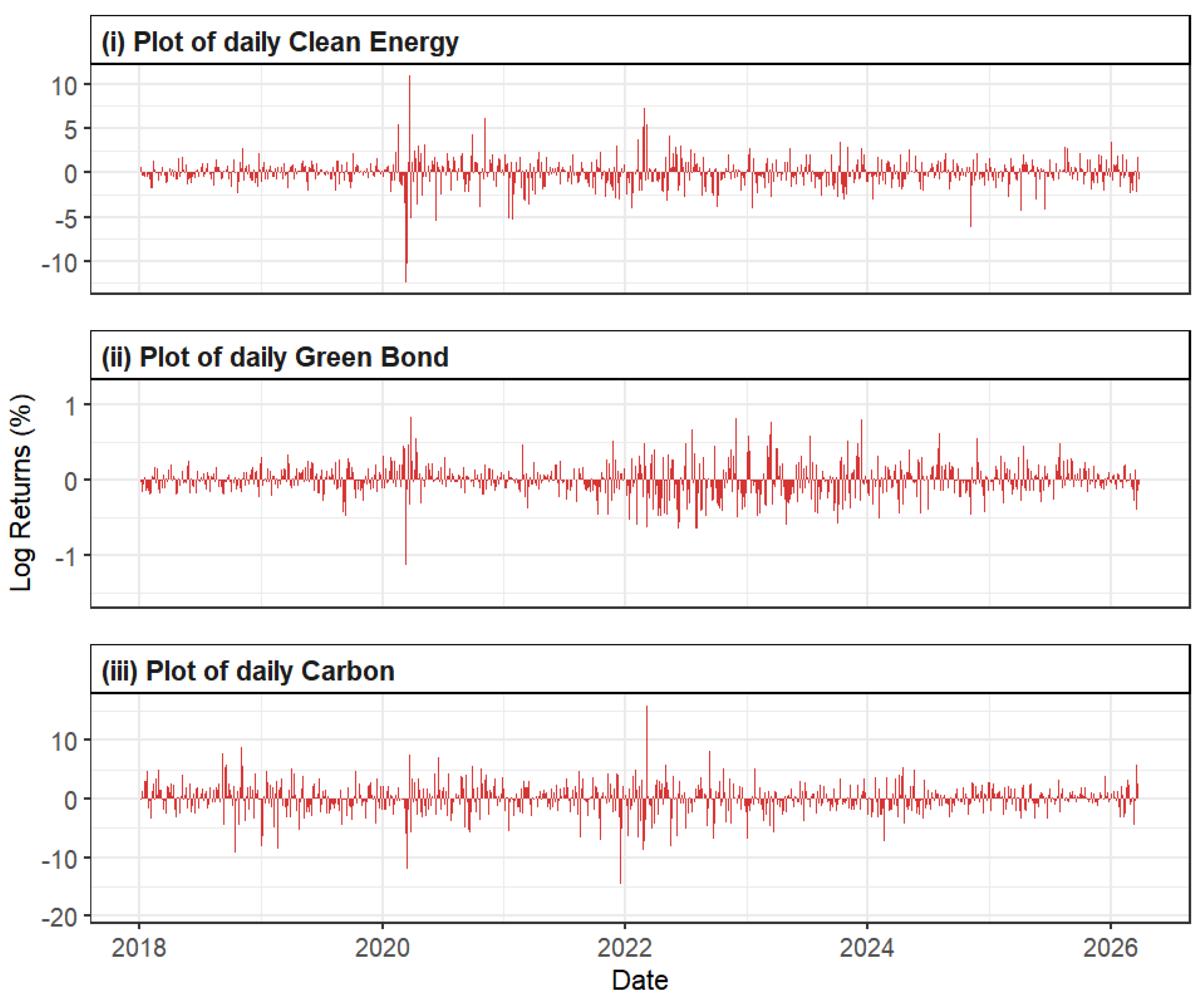
Figure 1 and Figure 2 plot the transformed SBI and green-finance return series, respectively. The SBI panels reveal episodic bursts of volatility, particularly around the pandemic and post-pandemic adjustment period, while the green-finance series also display visible clustering and tail events. Carbon is clearly the most volatile green submarket, whereas green bonds are comparatively smoother. These visual patterns already suggest that connectedness is likely to be nonlinear and concentrated in stressed states rather than under normal conditions.
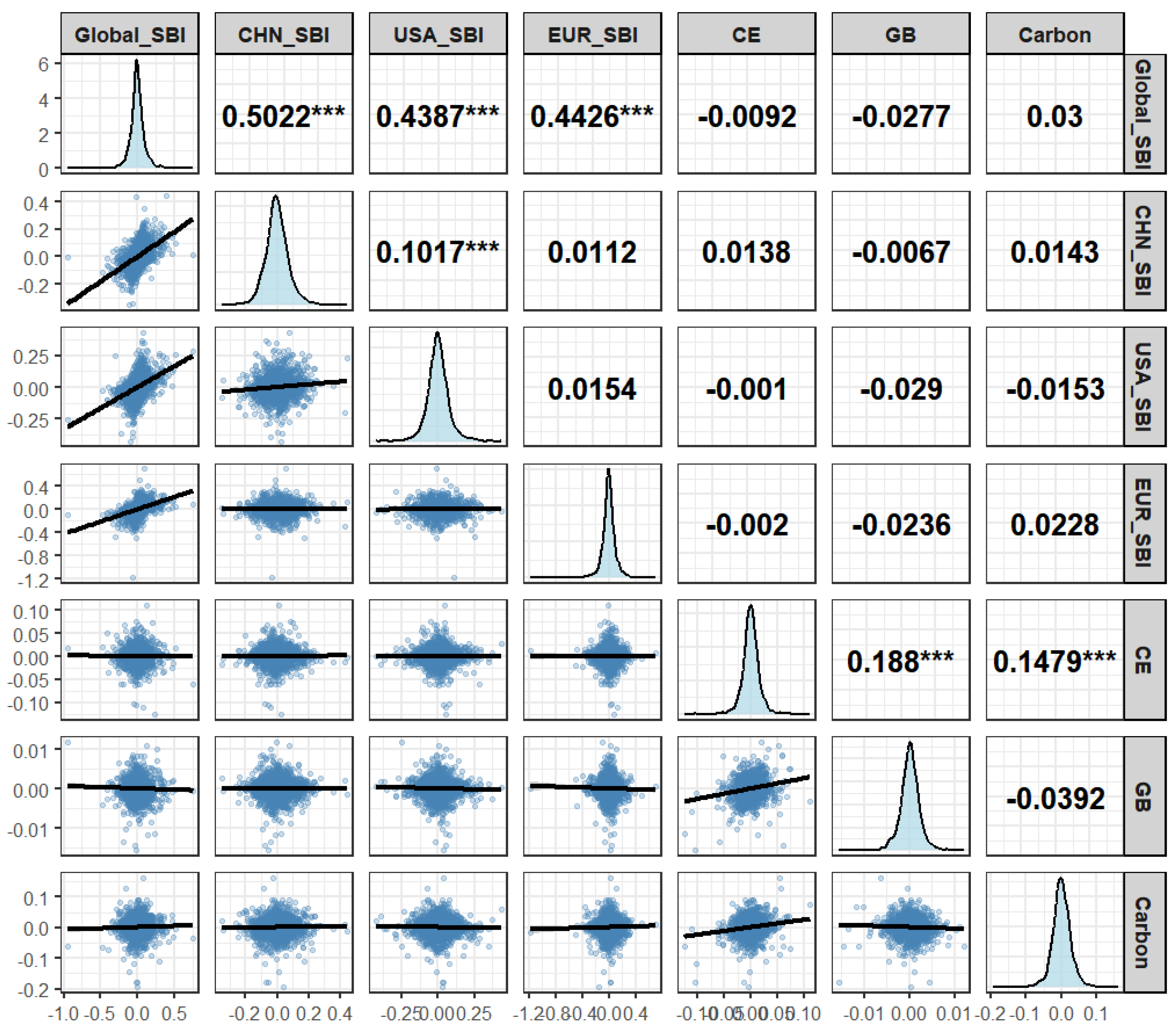
Table 2 reports the descriptive statistics of the transformed variables. All transformed series are stationary according to both the ADF and Phillips–Perron tests. The Jarque–Bera statistics strongly reject normality for every variable, confirming fat tails and non-Gaussian behavior. Among the supply chain indicators, the euro-area SBI is the most volatile (standard deviation 0.0977) and the most negatively skewed ( 0.8381 ), while the GSBI exhibits the highest average kurtosis among the aggregate measures. Within green finance, the carbon market has the largest mean return (0.0011) and standard deviation (0.0268), whereas green bonds are markedly less volatile (0.0023), a pattern consistent with earlier work showing that green bonds are usually less turbulent than equity- or commodity-linked green assets [17,26]. Table 3 further compares the raw SBI levels with the transformed SBI changes. The raw level series are more persistent and less uniformly stationary, whereas the transformed series strongly reject unit roots under both ADF and PP tests. This supports the use of transformed changes in the QQC estimation while preserving the economic interpretation that SBI changes measure innovations in bottleneck pressure. Figure 3 further shows that regional SBI changes and GSBI changes are positively and strongly correlated with one another, while contemporaneous linear correlations between supply bottleneck changes and green finance returns remain small. This combination of strong within-block dependence and weak cross-block linear correlation motivates the use of a state-dependent connectedness framework rather than a mean-based linear approach.
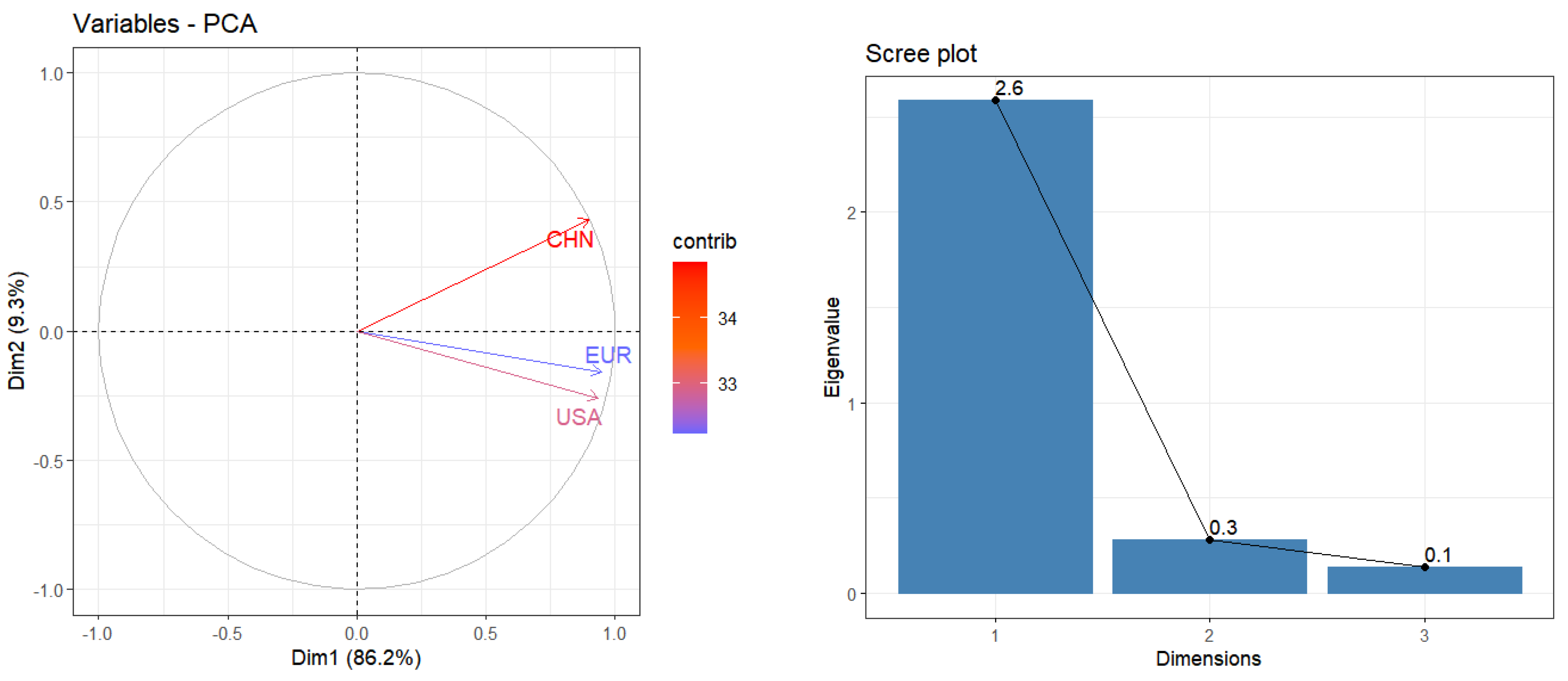
Because the three regional SBI level series are highly correlated, we extract their first principal component to construct the GSBI. The regional SBI levels are first standardized, and PCA is applied to the standardized level series. Table 4 shows that the first principal component has an eigenvalue of 2.5852 and explains 86.17% of the total variance, indicating that it captures the dominant common variation in regional supply bottlenecks. The sign of the first component is normalized so that it is positively correlated with the cross-regional average SBI, meaning that a higher G S B I represents stronger common bottleneck pressure. The resulting global factor is then first-differenced before QQC estimation because the standardized factor can take positive or negative values. The PCA loading plot in Figure 4 further shows that the three regional level series load positively and strongly on the first factor, supporting its interpretation as a global supply chain bottleneck indicator. As a transparency check, Section 4.4 also replaces the PCA factor with a simple standardized average of the regional SBI series.

3.2. Methodology

Supply bottlenecks are external disturbances whose financial effects are likely to be time-varying, nonlinear and state-dependent. To capture this feature, we adopt the quantile-on-quantile connectedness (QQC) approach, which maps connectedness across the quantile space and allows net connectedness positions to vary across calm, normal, and stressed regimes [32,33,41,42]. This is preferable to mean-based linear models because our objective is to identify how supply-side stress reconfigures green-finance connectedness in the tails as well as in intermediate states [43]. Our empirical design proceeds in two steps: we first extract a global supply bottleneck factor from the regional SBI series, and we then estimate pairwise QQC connectedness between each supply indicator and each green finance submarket.

3.2.1. Construction of the Global Supply Chain Shock Index

In addition to the regional supply bottleneck indicators for China, the United States, and the euro area, we construct a composite global supply chain shock index in order to capture the common component of supply-side stress across major production regions. Let S B I t C H N , S B I t U S A , and S B I t E U R denote the regional daily supply bottleneck indices. Since these series are highly correlated, we extract the first principal component from the standardized regional indicators. The resulting factor is interpreted as the global supply chain shock index:
G S B I t = PC 1 S B I t C H N , S B I t U S A , S B I t E U R .
This procedure yields a parsimonious measure of common global supply bottlenecks while preserving the regional information needed for the subsequent heterogeneity analysis. Because PCA is a linear dimension-reduction method, it may smooth some tail-specific co-movement in the regional SBI series. We therefore treat PCA as the baseline GSBI construction rather than as the only possible representation of global bottleneck pressure. Section 4.4 reports two alternative GSBI constructions: a simple standardized regional average and a quantile-rank GSBI. The latter first maps each regional SBI level into an inverse-normal empirical quantile score, averages the three quantile scores, and then takes first differences. This provides a nonlinear, rank-based aggregation that gives additional weight to regional tail positions. Accordingly, the empirical analysis is conducted at two levels: first, using the GSBI; and second, using each regional supply bottleneck indicator separately.

3.2.2. Quantile-on-Quantile Connectedness Framework

To examine the nonlinear, asymmetric, and state-dependent connectedness between supply chain disturbances and green finance markets, this paper employs the QQC approach proposed by Gabauer and Stenfors [33] and applied in a pairwise supply-chain setting by Youssef et al. [32]. The main advantage of this framework is that it allows the connectedness intensity between two variables to vary jointly across their quantiles. Hence, the method is particularly suitable for the present setting, where the connectedness between supply chain bottleneck indicators and green finance assets may differ substantially across bearish, normal, and bullish market conditions.
The empirical application is implemented in a bivariate pairwise manner. For each supply chain shock indicator m { G S B I , S B I C H N , S B I U S A , S B I E U R } and each green finance submarket n { C E , G B , C a r b o n } , we define the 2 × 1 vector
x t ( m , n ) = s t ( m ) g t ( n ) ,
where s t ( m ) denotes the return of the selected supply chain shock indicator and g t ( n ) denotes the return of the corresponding green finance market variable, namely clean energy equities ( C E ), green bonds ( G B ), or the carbon market ( C a r b o n ).
For each pair, the QQC framework starts from a quantile vector autoregression, Q V A R ( p ) , defined as
x t = μ ( τ ) + j = 1 p B j ( τ ) x t j + u t ( τ ) ,
where x t is a K × 1 vector of endogenous variables, with K = 2 in the present application, τ = ( τ 1 , τ 2 ) is a vector of quantiles with τ k ( 0 , 1 ) , μ ( τ ) is a K × 1 vector of quantile-specific intercepts, B j ( τ ) is a K × K matrix of quantile-specific autoregressive coefficients, and u t ( τ ) is a K × 1 vector of innovations with variance–covariance matrix H ( τ ) .
Using the Wold representation theorem, the Q V A R ( p ) system can be written in its quantile vector moving average representation:
x t = μ ( τ ) + h = 0 A h ( τ ) u t h ( τ ) ,
where A h ( τ ) is the quantile-specific impulse response coefficient matrix at horizon h.
Based on this representation, the F-step-ahead generalized forecast error variance decomposition (GFEVD) is computed as
ϕ i j , τ g ( F ) = h = 0 F 1 e i A h ( τ ) H ( τ ) e j 2 / H j j ( τ ) h = 0 F 1 e i A h ( τ ) H ( τ ) A h ( τ ) e i ,
where e i is a selection vector with unity in the ith position and zeros elsewhere. Since the rows of the generalized variance decomposition do not necessarily sum to one, we follow Diebold and Yilmaz [43] and normalize the decomposition as
ϕ ˜ i j , τ g ( F ) = ϕ i j , τ g ( F ) k = 1 K ϕ i k , τ g ( F ) .
The scaled GFEVD is then used to construct the standard connectedness measures. The directional connectedness to others from variable i is given by
C i , τ T O ( F ) = k = 1 k i K ϕ ˜ k i , τ g ( F ) ,
while the directional connectedness from others to variable i is
C i , τ F R O M ( F ) = k = 1 k i K ϕ ˜ i k , τ g ( F ) .
The net connectedness of variable i is defined as the difference between outgoing and incoming connectedness:
C i , τ N E T ( F ) = C i , τ T O ( F ) C i , τ F R O M ( F ) .
A positive value of C i , τ N E T ( F ) indicates that variable i occupies a positive net connectedness position, whereas a negative value implies that incoming connectedness dominates outgoing connectedness for that variable.
Finally, the adjusted total connectedness index (TCI), which measures the overall level of bilateral interconnectedness at quantile pair τ , is computed as
T C I τ ( F ) = K K 1 · 1 K i = 1 K C i , τ F R O M ( F ) .
The larger the value of T C I τ ( F ) , the stronger the degree of bilateral connectedness within the corresponding two-variable system.

3.2.3. Diagonal- and Anti-Diagonal-State Quantile Connectedness

A key feature of the QQC framework is that it distinguishes between diagonal-state and anti-diagonal-state quantile connectedness. Diagonal-state connectedness refers to quantile combinations in which both variables are simultaneously in similar market states, such as lower–lower, median–median, or upper–upper quantiles. In contrast, anti-diagonal-state connectedness refers to quantile combinations in which one variable is in a low state while the other is in a high state, or vice versa.
Formally, diagonal-state connectedness is associated with quantile pairs satisfying τ 1 = τ 2 , whereas anti-diagonal-state connectedness is associated with quantile pairs lying on the anti-diagonal of the quantile space, i.e., τ 1 = 1 τ 2 . This distinction is particularly useful when the interaction between two variables changes across market states or when the relationship is asymmetric. In the context of this paper, it allows us to identify whether supply chain shocks are most strongly connected with green finance markets when both are under stress, when both are tranquil, or when one is stressed while the other is not.
For each rolling window, the QQC approach produces a full quantile-on-quantile connectedness surface over the grid
T = { 0.05 , 0.275 , 0.50 , 0.725 , 0.95 } × { 0.05 , 0.275 , 0.50 , 0.725 , 0.95 } .
This five-point empirical grid captures lower-tail, intermediate, median, and upper-tail states while preserving rolling-window estimation stability. In the empirical section, we report (i) average total and net connectedness over the quantile surface, and (ii) time-varying diagonal- and anti-diagonal-state total connectedness in order to evaluate how state-dependent connectedness evolves across major episodes of global stress.

3.2.4. Estimation Strategy

The QQC measures are estimated in a rolling-window framework in order to capture the time variation in the connectedness structure. Following the empirical design of Gabauer and Stenfors [33] and Youssef et al. [32], the baseline specification is based on a 200-day rolling-window Q V A R ( τ ) model with a lag length selected by the Bayesian Information Criterion (BIC) and a 20-step-ahead forecast horizon. With daily data, a 20-step horizon approximately corresponds to a one-month forecasting window and provides a natural benchmark for medium-run spillover analysis.
For each rolling window, the analysis is repeated for all pairwise combinations between the four supply chain shock indicators and the three green finance market variables. Accordingly, the empirical design consists of twelve pairwise QQC systems:
{ G S B I , S B I C H N , S B I U S A , S B I E U R } × { C E , G B , C a r b o n } .
This pairwise structure is deliberate. It allows us to isolate the connectedness between each source of supply-side stress and each green finance submarket, thereby facilitating a transparent comparison of state-dependent and region-specific patterns. It also imposes an important boundary on interpretation. The pairwise QQC estimates describe bilateral state-dependent connectedness conditional on the estimated bivariate QVAR; they do not by themselves identify structural causality or fully partial out common drivers such as monetary policy, energy prices, inflation news, global risk sentiment, or climate-policy news. For this reason, the empirical discussion uses the terms “connectedness”, “net connectedness”, and “state-dependent dependence” when referring to the estimated results, and treats outgoing–incoming roles as model-implied connectedness positions rather than as causal effects.
The empirical analysis proceeds in two stages. In the first stage, we investigate the connectedness between the GSBI and each green finance submarket in order to establish the baseline relationship between global supply-side stress and the selected green-finance pairs. In the second stage, we replace the GSBI with the regional supply bottleneck indices for China, the United States, and the euro area, respectively, in order to uncover regional heterogeneity in the connectedness mechanism.

3.2.5. Interpretation in the Context of Green Finance

In the present setting, the QQC framework is used to examine how supply bottleneck indicators are associated with changes in the connectedness structure of the green finance market. Clean energy equities represent the valuation side of the green transition, green bonds represent the financing side, and the carbon market captures the regulatory-pricing side. By estimating total, directional, and net connectedness across quantile states, the methodology allows us to identify which green finance submarket is most sensitive to supply-side disturbances, whether supply indicators occupy positive or negative net connectedness positions, and whether these roles vary across normal and extreme market conditions.
The baseline implementation uses five quantiles, { 0.05 , 0.275 , 0.50 , 0.725 , 0.95 } , a 200-day rolling window, a 20-step-ahead forecast horizon, and one QVAR lag. The quantile grid is chosen to cover lower-tail, intermediate, median, and upper-tail states while keeping the rolling QVAR estimation stable in daily data. The 200-day window approximates a trading-year information set, the 20-step horizon captures roughly one trading month of forecast-error connectedness, and the one-lag QVAR is selected by the benchmark lag-choice procedure and is consistent with the daily QQC literature. Section 4.4 reports additional checks using 150- and 250-day rolling windows and 10- and 30-step forecast horizons.
Consequently, the QQC approach is particularly well suited to the objectives of this paper. It captures nonlinear and asymmetric connectedness and provides a state-contingent view of how an external real-economy disturbance is associated with changes in the internal connectedness structure of a green financial system.

4. Empirical Results

4.1. Global Supply Chain Shock and Green Finance Markets

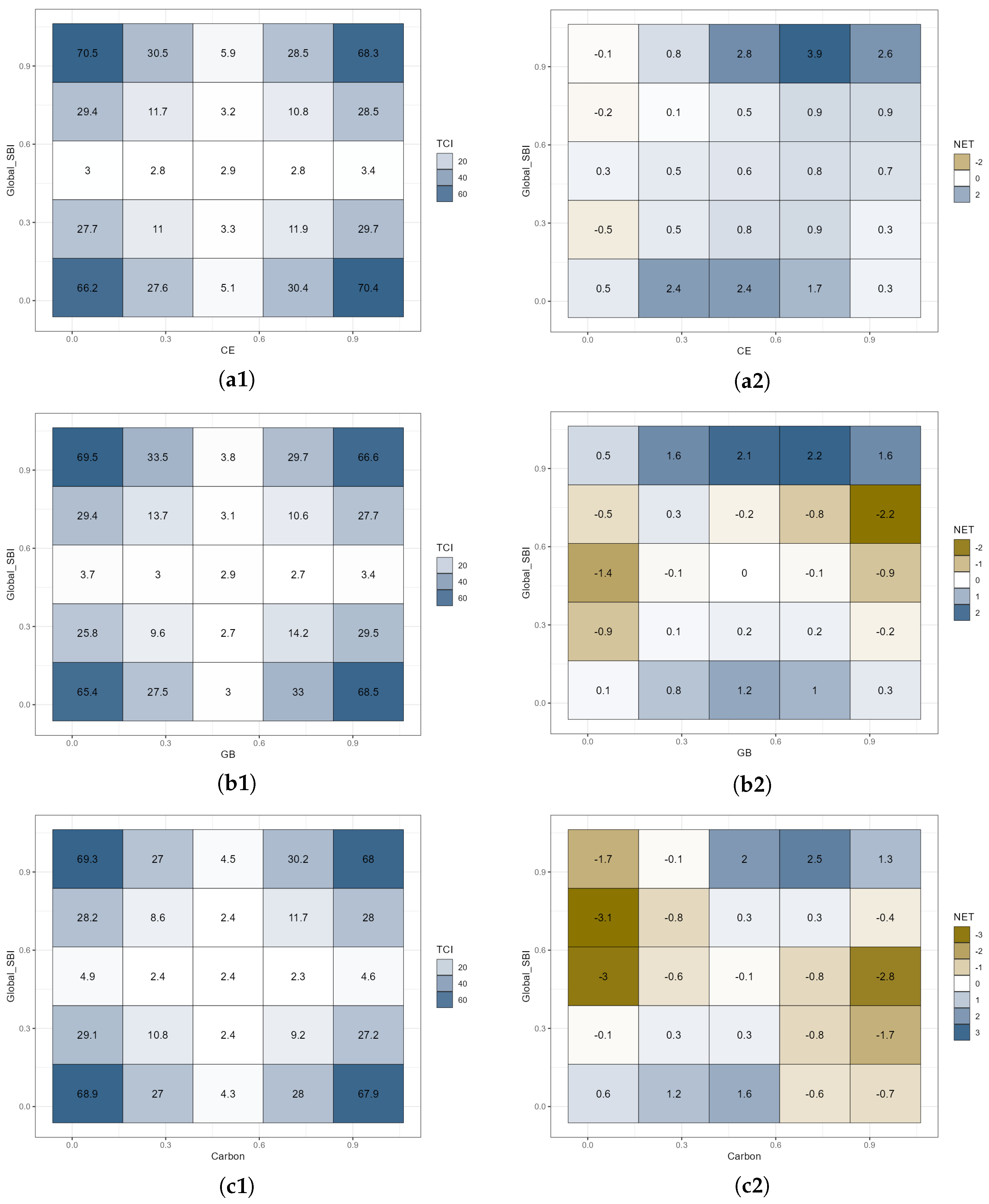
Figure 5 and Figure 6 report the average and dynamic quantile-on-quantile connectedness between the GSBI and the three green-finance submarkets. A common feature across all three pairs is the clear state dependence of connectedness. Average total connectedness is weak around the middle of the joint distribution, where the TCI is mostly between 2 and 5, but rises sharply in the tails and at cross-tail combinations. For CE, the strongest linkages appear at the joint upper-tail state (70.5) and at the lower-GSBI/higher-CE state (70.4). For GB, the highest values are 69.5 and 68.5 at the joint lower and lower-GSBI/higher-GB cells, while Carbon reaches 69.3 and 68.9 at the joint lower and lower-tail GSBI states. This U-shaped connectedness surface indicates that global supply bottlenecks matter most when the bilateral system is under stress and much less under normal market conditions. The result is consistent with the broader connectedness literature showing that tail-state connectedness is typically much stronger than that observed around the center of the distribution [25,26,32].
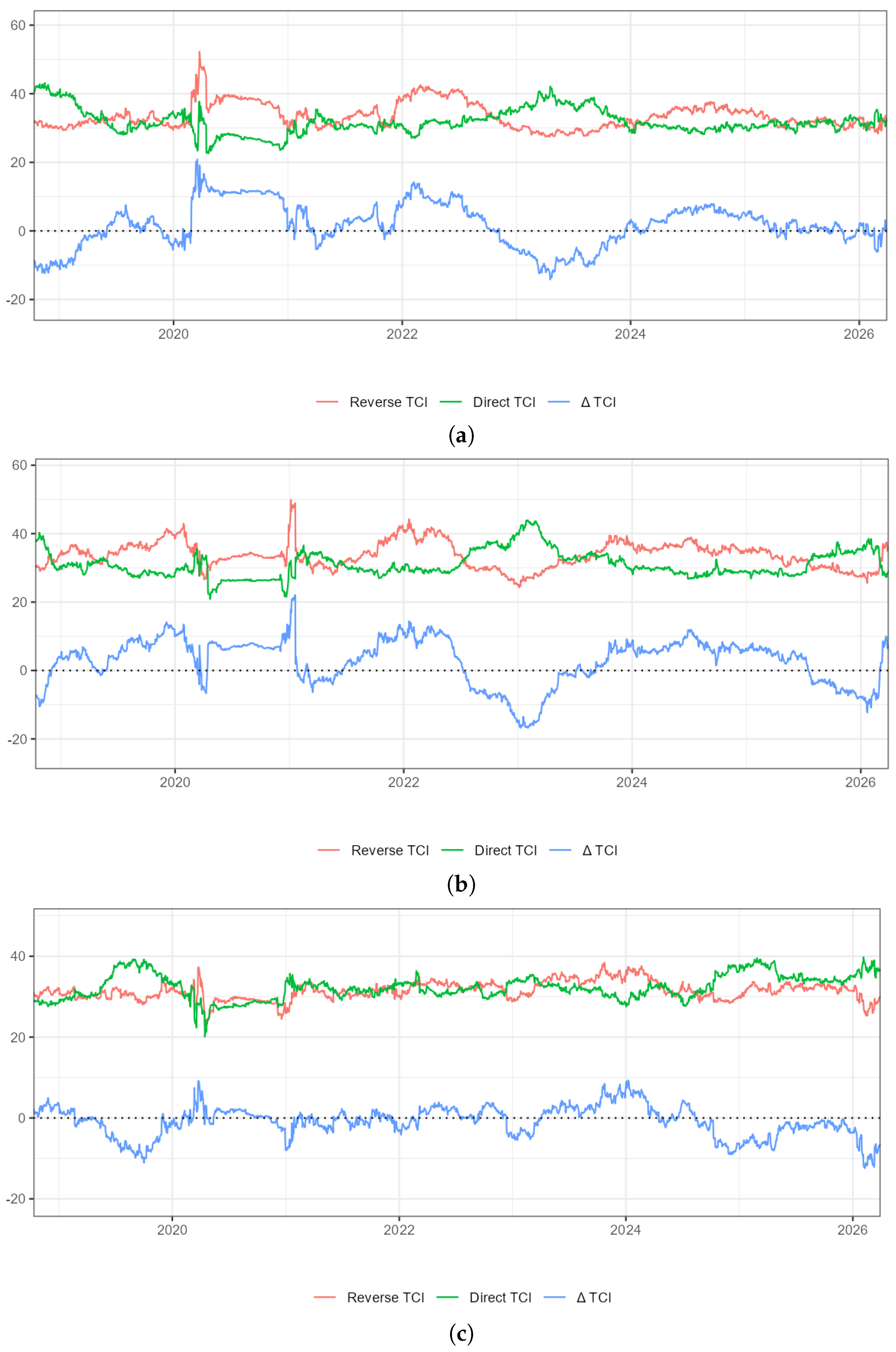
For CE, the net surface is predominantly positive, especially in the upper part of the quantile space and along several cross-tail cells. This means that the GSBI generally occupies a positive net connectedness position relative to clean energy equities, with the strongest net effect emerging when the GSBI is high and CE is also in a high state. The dynamic results confirm this asymmetry but also show that the pattern is not constant through time. Before 2020, the blue net line is mostly negative, indicating episodes in which CE occupied the stronger net connectedness position in the bilateral system. During the COVID-19 pandemic and the subsequent adjustment period, net connectedness associated with the GSBI strengthens materially, and the net line turns positive for sustained intervals.
The GB pair displays a more mixed net pattern. The GSBI has a positive net connectedness position at the lower- and upper-tail states and in several middle-to-upper GB cells, but negative values emerge when the GSBI is in the upper-middle range and GB is in a strong upper-tail state. In dynamic terms, the blue net line oscillates around zero far more often than in the CE case. Periods of positive net connectedness for the GSBI relative to GB are interspersed with clear reversals, particularly around 2022–2023, implying that the green bond market alternates between weaker and stronger net connectedness positions in the bilateral system.
Carbon exhibits the most distinctive net pattern under the GSBI. Although average total connectedness still becomes very large in tail states, the net heatmap is dominated by negative values across much of the middle and upper-middle GSBI range, with only a few positive pockets when the GSBI is very low or when Carbon is in the middle-to-upper quantiles. The dynamic results are consistent with this picture: the net line remains negative for long stretches, interrupted only by brief positive episodes around 2020 and again later in the sample. Hence, the carbon market frequently occupies the stronger net connectedness position in the GSBI bilateral system once pricing, regulation, and market expectations adjust [23,26]. Economically, this feedback-type connectedness should not be read as direct structural causality from carbon futures to physical bottlenecks. It is more plausibly interpreted as a mixture of carbon-pricing feedback and common macro-financial forces. Carbon-price volatility can reflect energy-cost pressure, climate-policy news, geopolitical disruptions, and expected compliance costs, all of which can also alter firms’ expectations about production costs, delivery schedules, and input substitution. This interpretation is consistent with evidence that EU ETS prices are shaped by allowance-market design, electricity-sector pass-through, compliance expectations, and policy credibility [44,45], as well as with the European Commission’s discussion of ETS price transmission through electricity-related production costs and inflation assumptions [46].
The dynamic results in Figure 6 reinforce these conclusions. For CE and GB, the blue net-connectedness line turns positive during the COVID-19 pandemic and remains positive for long stretches through the post-pandemic adjustment period, indicating that the GSBI occupied a stronger positive net connectedness position in those episodes. A second wave of stronger diagonal-state connectedness appears around 2022, a period that also included the Russia–Ukraine war and associated energy, shipping, and commodity-market disruptions. This timing provides useful macro-financial context, but the QQC design does not identify those events as structural causes of the estimated connectedness patterns. For Carbon, the blue line remains closer to zero and is frequently negative, meaning that the carbon market often occupies the stronger feedback-type connectedness position rather than merely being associated with supply-side stress. Late-sample fluctuations can also be read against the background of renewed tensions in the Middle East and concerns over shipping and energy transit, although the short end-of-sample window warrants caution in interpretation. Taken together, the global results suggest that supply chain disruptions tighten bilateral connectedness with green-finance markets primarily in the tails and that the supply indicator often occupies a positive net connectedness position under stressed conditions. Furthermore, the carbon market occupies a more endogenous and strategically important position than the other two green submarkets, a pattern that echoes earlier findings on green-finance connectedness [23,26,27]. Because energy prices, monetary policy, geopolitical conflict, and climate-policy news may simultaneously affect both carbon prices and supply-chain indicators, these negative net-connectedness patterns are interpreted as model-implied connectedness positions rather than as evidence of literal reverse causality.

4.2. Regional Supply Chain Shocks and Green Finance Markets

4.2.1. China Supply Chain Shocks and Green Finance Markets

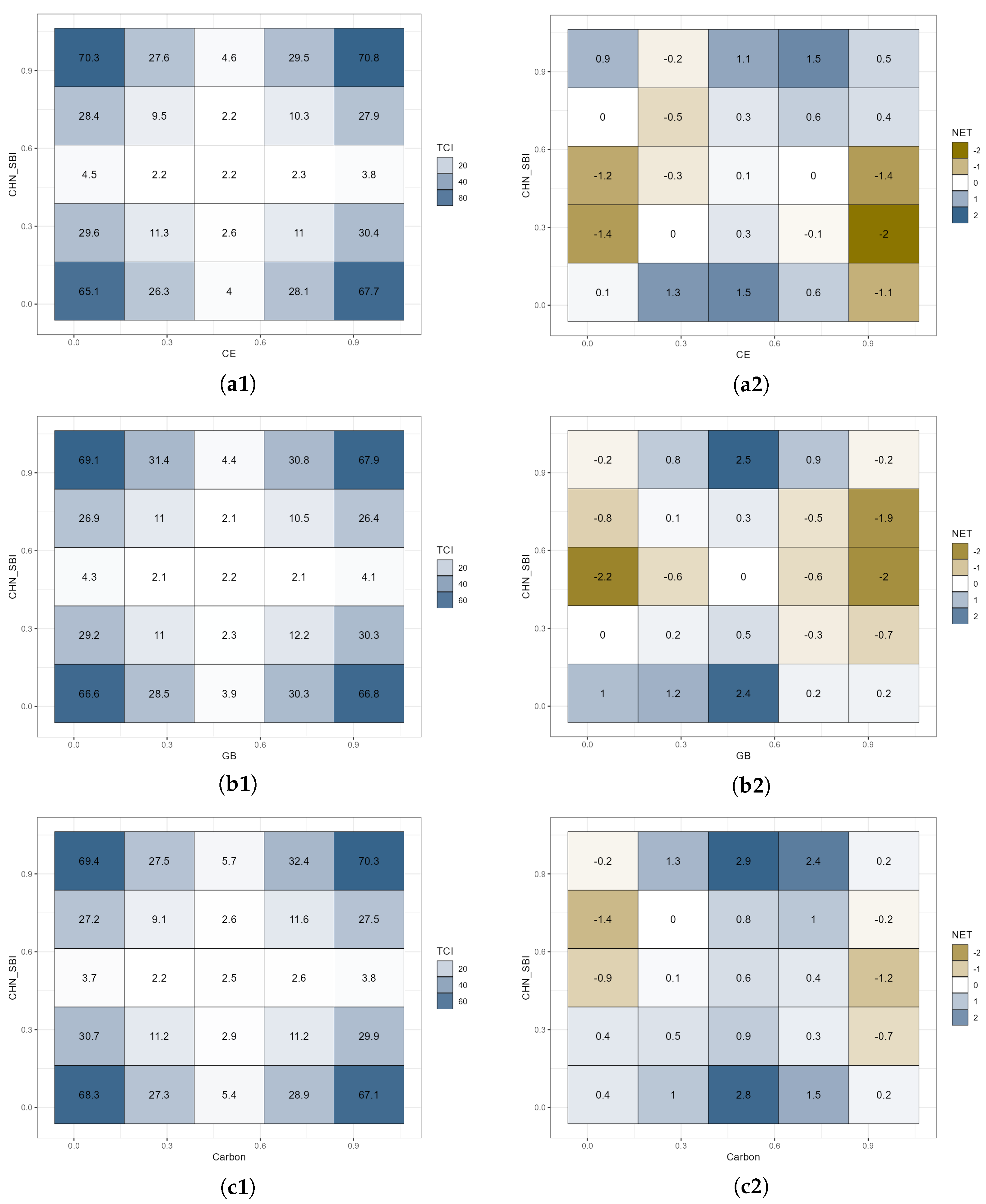
Figure 7 and Figure 8 show that Chinese supply bottlenecks are strongly connected with all three green-finance segments in extreme states. Average total connectedness is again U-shaped. The largest values are observed in the upper-tail and cross-tail cells, reaching 70.8 for CHN SBI and CE, 69.1 for CHN SBI and GB, and 70.3 for CHN SBI and Carbon. By contrast, connectedness in the center of the distribution is very weak, mostly around 2–4. This pattern suggests that Chinese supply-side stress becomes most relevant for green-finance connectedness during episodes of pronounced market imbalance.
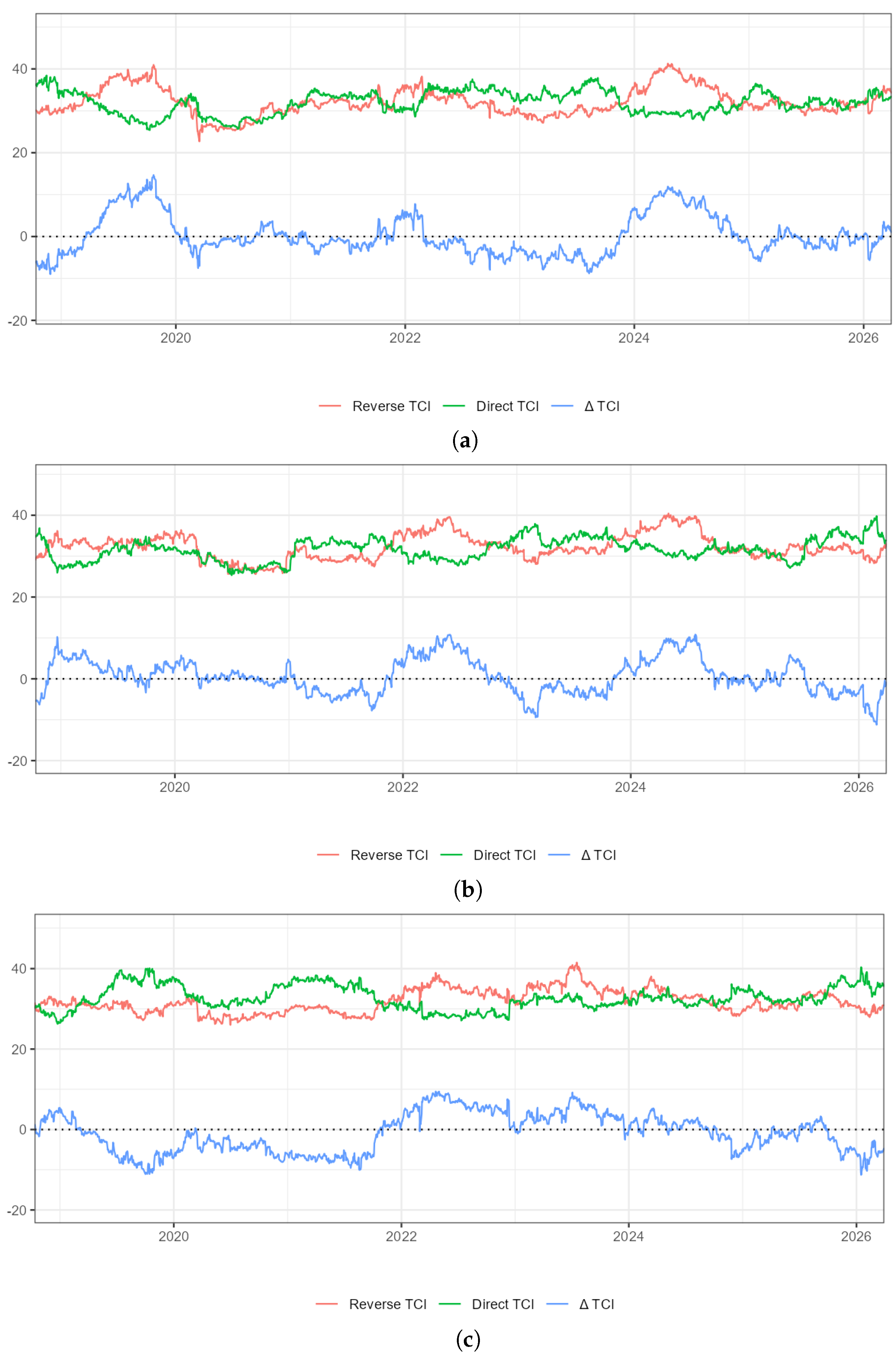
For CE, the net heatmap is mixed but leans positive in the upper-right portion of the quantile space, indicating that CHN SBI tends to occupy a stronger net connectedness position relative to clean energy equities when both variables are in relatively strong states. Negative values appear mainly when CE is in the far upper tail while CHN SBI is in lower-to-middle states. The dynamic plot reinforces this interpretation: the net line rises sharply around 2019–2020, turns negative or near zero through parts of 2021–2023, and becomes positive again later in the sample. Thus, China-related supply stress is an important but time-varying correlate of clean-energy connectedness. The sharp increase around 2020 can be read against the background of China’s central role in global manufacturing networks during the COVID-19 disruption, while the renewed positive phases after 2022 are consistent with a period in which Asian production bottlenecks and global repricing of energy-transition assets became especially salient [20,23]. These event references are used as contextual interpretation rather than as causal evidence from the QQC design.
For GB, the average net surface is more balanced and displays stronger sign reversals. Positive cells cluster when CHN SBI is in the lower tail, whereas negative values dominate several middle and upper-middle quantile combinations, especially when GB itself is in a weak or very strong state. The dynamic series likewise oscillates around zero for much of the sample, with only short-lived episodes in which Chinese bottlenecks occupy the stronger net connectedness position. This implies that the green bond market is more buffered than CE and that the bilateral relation with CHN SBI is characterized by alternating net connectedness positions rather than persistent one-way dominance. This more balanced pattern is broadly in line with studies showing that green bonds often occupy a comparatively defensive or receiver-like role within green financial systems [17,18,26].
For Carbon, the strongest average connectedness is again found in the tails, but the net structure differs from both CE and GB. Positive net values are concentrated when CHN SBI is in the lower tail and Carbon is in the middle-to-upper range, while negative values emerge when CHN SBI is in upper-middle states or when Carbon is weak. The dynamic net line is mostly negative before 2021, turns positive around 2022, and then moves back toward zero. This pattern suggests that the carbon market sometimes has a weaker net connectedness position relative to Chinese supply bottlenecks, but it can also occupy the stronger net position once carbon pricing adjusts to broader market expectations. The positive phase around 2022 is consistent with a period of elevated energy and compliance-cost repricing, which provides context for the feedback role of carbon pricing in green finance connectedness [23,26].

4.2.2. U.S. Supply Chain Shocks and Green Finance Markets

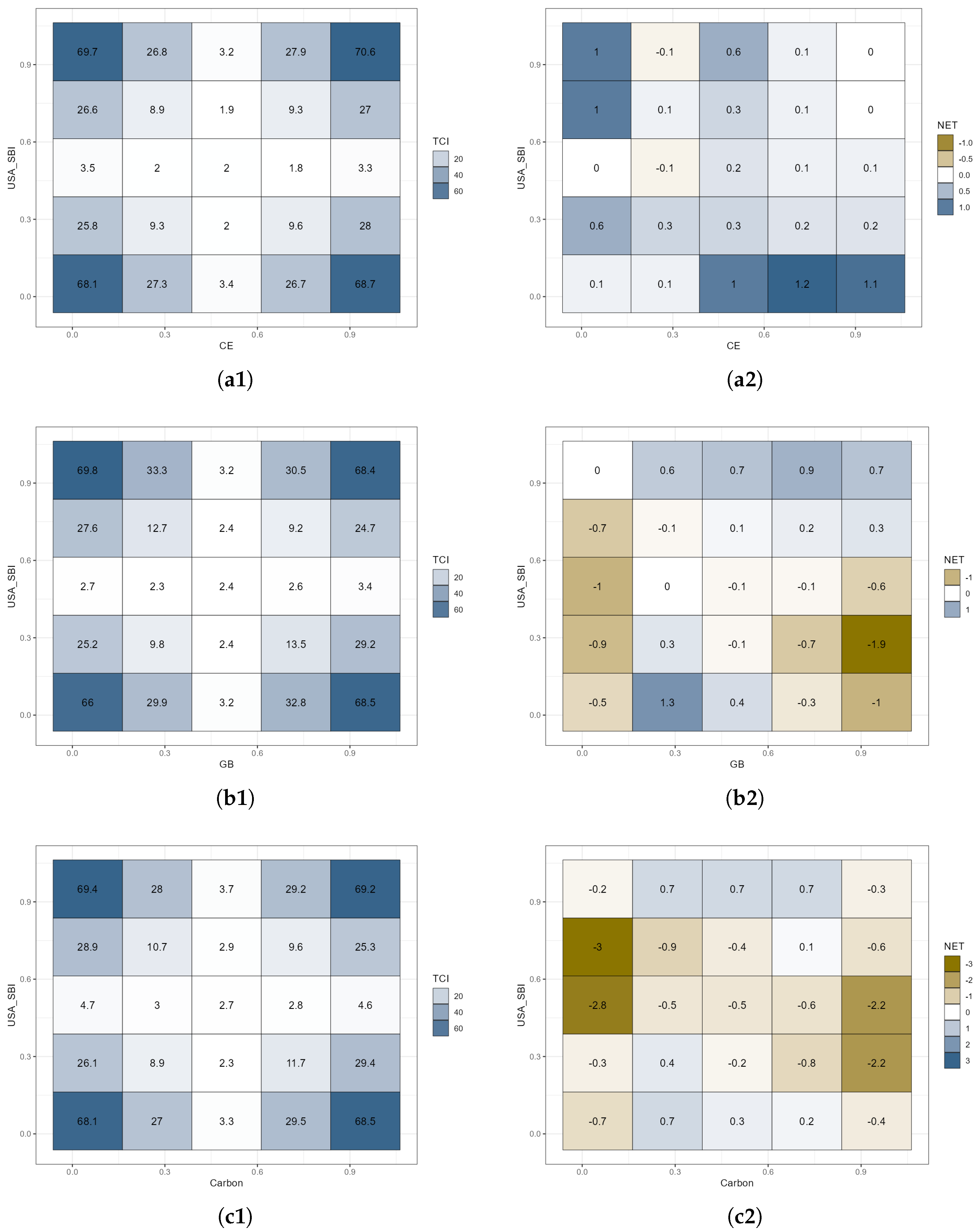
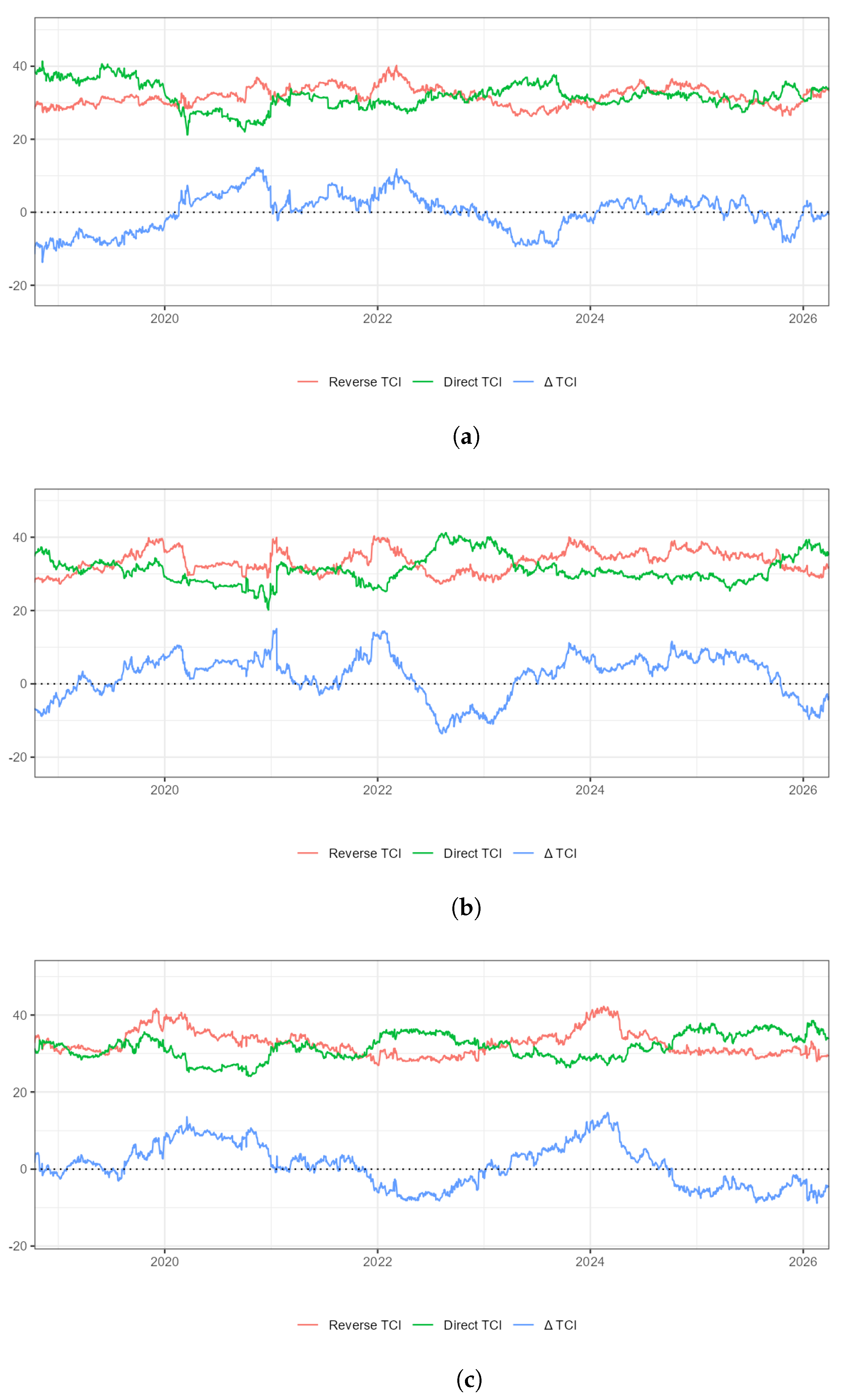
Figure 9 and Figure 10 reveal similarly strong tail dependence for U.S. supply bottlenecks. Average total connectedness is largest at the corners of the quantile space and falls back to values close to 2–5 in the middle quantiles. CE reaches a peak TCI of 70.6, GB 69.8, and Carbon 69.4, indicating that U.S. supply-side stress becomes tightly connected with all three green-finance markets in extreme states.
For CE, the net heatmap is overwhelmingly positive except for a few cells with very small negative values. This means that USA SBI has the stronger net connectedness position relative to clean energy equities across most quantile combinations, especially when both variables lie in the lower or upper tails. The dynamic evidence is consistent with this result. The net line is negative early in the sample, but it turns positive for a long interval around 2020–2022 and thereafter fluctuates around zero with several positive bursts. Overall, CE is the green-finance market most persistently associated with U.S. supply bottlenecks. The long positive phase around 2020–2022 is consistent with a period that included pandemic-related shortages, semiconductor bottlenecks, and energy-market repricing, while late-sample bursts can be read against the background of renewed geopolitical tensions affecting energy and shipping routes. The result is consistent with the view that clean-energy valuations respond quickly to externally induced stress in production and input markets [23,27].
For GB, the net structure is much less one-sided. Positive values dominate the upper-tail row and some lower-tail cells, but negative values appear in the middle of the quantile space and become especially strong when GB is in its upper tail while USA SBI is not. The dynamic net line also alternates repeatedly between positive and negative territory, with a pronounced negative phase around 2022 and renewed positive connectedness thereafter. This indicates that the U.S. supply chain shock–green bond relation is highly regime-dependent and cannot be characterized as stable one-way dominance. The pronounced negative phase around 2022 is consistent with a macro-financial setting in which interest-rate expectations, energy costs, and project-financing conditions were being repriced, temporarily strengthening the feedback role of the green bond market in the bilateral system [18,24,26].
For Carbon, the average net heatmap is mostly negative. Large negative values appear when USA SBI is in the middle or upper-middle quantiles and Carbon is in either tail, while only a handful of cells in the upper row remain positive. The time-varying results strongly support this finding: the net line stays below zero for most of the sample, except for brief upward movements around 2019–2020 and 2024. Therefore, relative to the U.S. supply bottleneck indicator, the carbon market more often has the stronger net connectedness position, suggesting a stronger role for market pricing and policy expectations in this bilateral relation.

4.2.3. Euro Area Supply Chain Shocks and Green Finance Markets

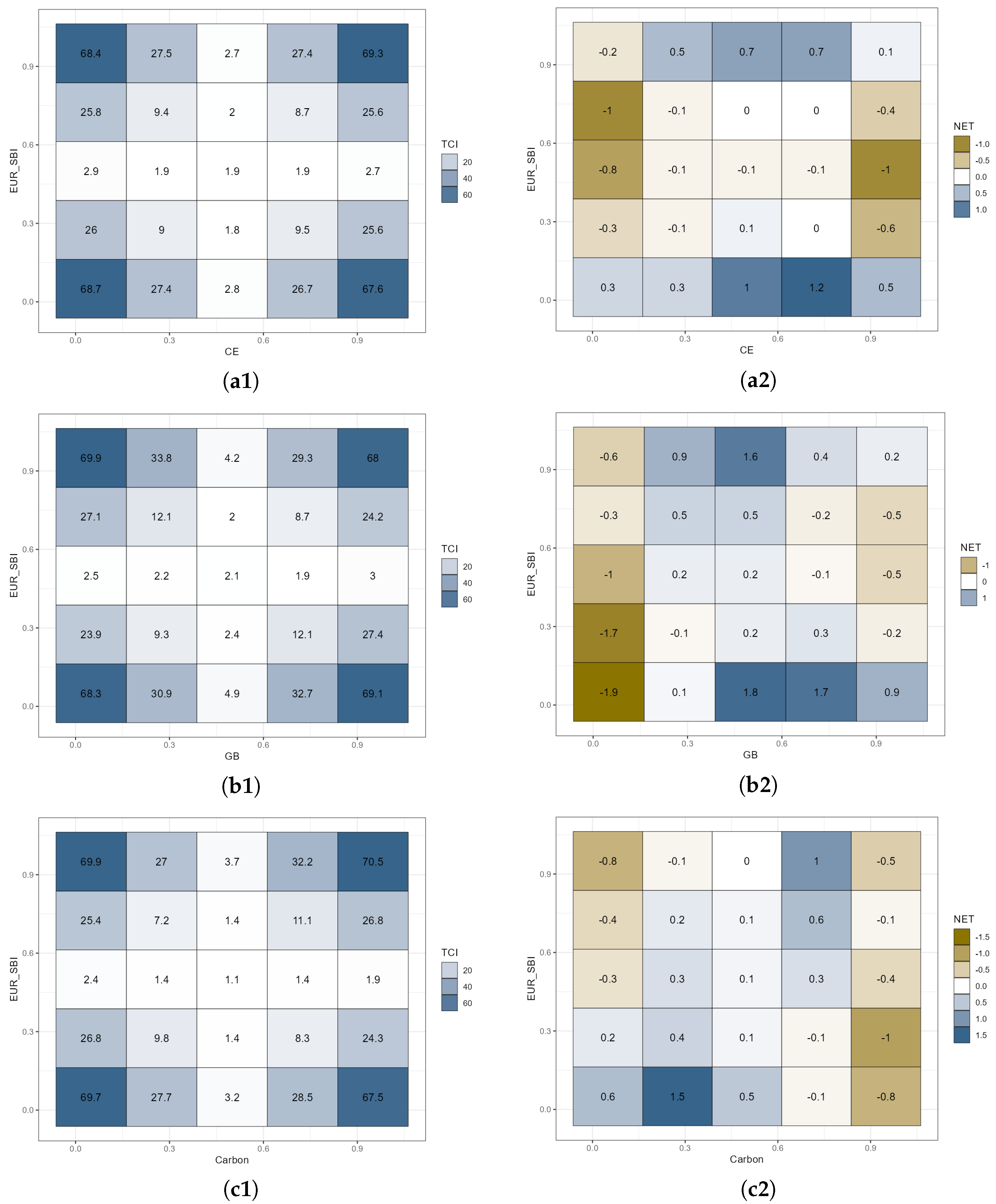
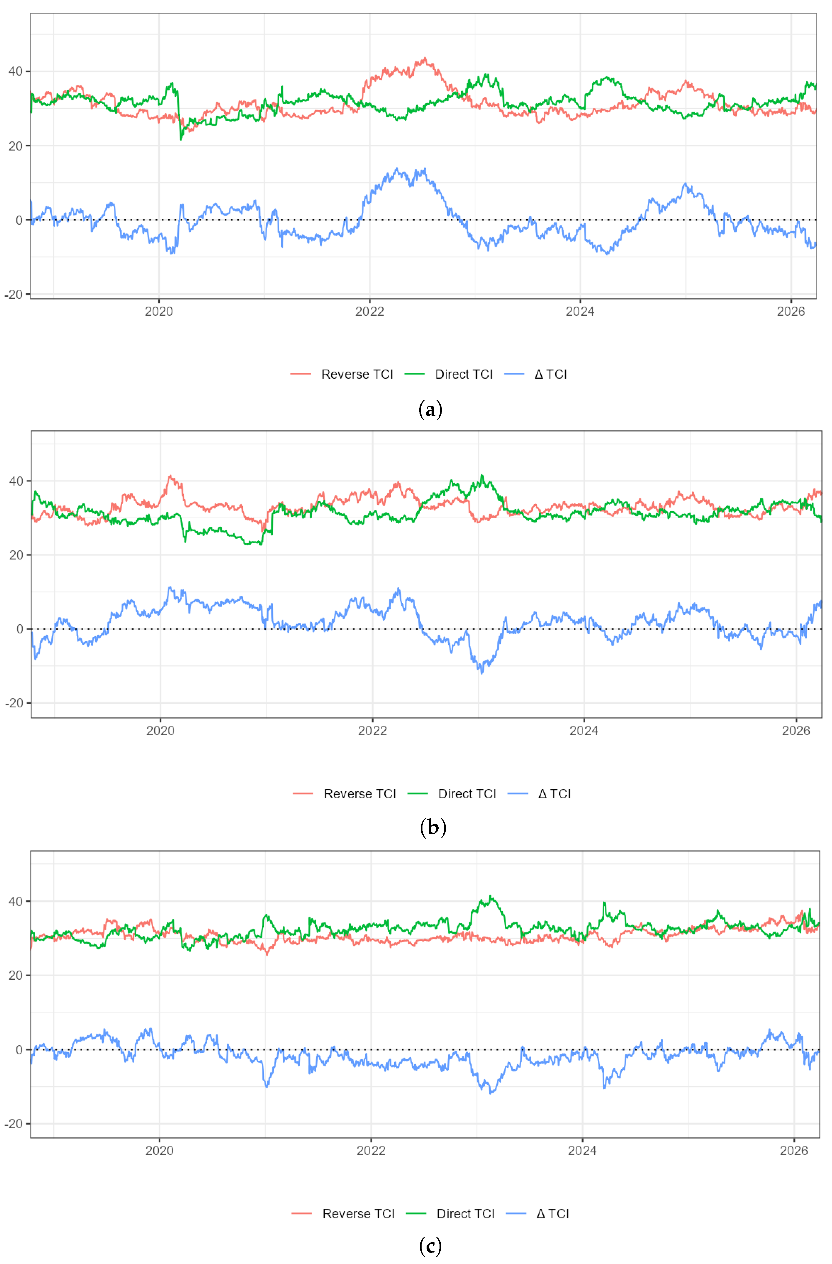
Figure 11 and Figure 12 indicate that euro-area supply bottlenecks are also strongly connected with green finance in tail states, albeit with a milder and more balanced pattern than for China or the United States. The largest average total connectedness is observed for Carbon, where the joint upper-tail cell reaches 70.5. The corresponding peaks are 69.9 for GB and 69.3 for CE. In all three cases, middle-state connectedness remains very low, especially for Carbon, confirming that euro-area supply pressures matter mainly during stressed regimes.
For CE, the net heatmap is mixed and tilted slightly negative, with only a few positive cells concentrated in the lower-SBI row and the upper-tail CE states. The dynamic net line stays close to zero over much of the sample but rises sharply around 2022 and again later in the period. This means that euro-area bottlenecks only intermittently occupy the stronger net connectedness position relative to clean energy equities; for long intervals, CE itself remains equally important or stronger within the bilateral system.
For GB, the average net surface combines sizeable negative values in the lower-left part of the quantile space with clear positive pockets when EUR SBI is very low and GB is in the middle-to-upper range. In dynamic terms, the net line is positive through much of the early and middle sample, then turns negative around 2023 before moving back toward zero and mildly positive values. Relative to the Chinese and U.S. cases, the euro-area GB relation is more balanced, but it still shows that financing conditions can become temporarily more sensitive to euro-area bottlenecks during stress episodes [18,24].
For Carbon, the euro-area results are distinctive. Average total connectedness is strongest here, yet the net heatmap is dominated by small negative or near-zero values except when EUR SBI is in the lower tail. The dynamic net line also fluctuates narrowly around zero, with a more notable negative dip around 2022–2023 and only modest positive values at the end of the sample. Thus, the euro-area carbon pair is characterized by very strong tail-state coupling but relatively limited persistent net dominance, which is consistent with carbon prices and euro-area bottlenecks reacting jointly to common regional stress rather than one side consistently leading the other [23,26].

4.3. Comparative Discussion of Green-Finance Connectedness

A comparison across markets and regions reveals three broad features of the selected green-finance pairs. Table 5 summarizes the baseline connectedness patterns. First, connectedness is systematically state-dependent. For all four supply indicators and all three green-finance markets, average total connectedness is low in the center of the joint distribution but rises sharply in the tails. This confirms that supply-chain disruptions matter less as average background noise and more as stress-state correlates that tighten bilateral linkages when market conditions are unusually weak or strong.
Second, CE is the most consistently supply-sensitive green-finance segment. Under the global, Chinese, and especially U.S. indicators, CE frequently displays positive net values in upper-tail states, implying that supply bottlenecks often hold a stronger net connectedness position relative to the clean-energy equity market. This is consistent with the idea that the valuation channel of the green transition reacts quickly to disruptions in input availability, production expectations, and sentiment. The regional pattern is also economically intuitive. China’s bottleneck indicator is closely linked to clean-energy valuation because China occupies a central position in solar photovoltaic modules, battery materials, and renewable-energy equipment supply chains. The IEA reports that China’s share exceeds 80% in all major solar-panel manufacturing stages and that China supplies about 85% of cathode active materials and more than 90% of anode active material production [47,48]. U.S. bottlenecks matter for CE because U.S.-listed clean-energy firms are sensitive to technology-sector valuation, financing conditions, and policy expectations surrounding clean-energy investment. The IEA reports that the United States accounts for 15% of global clean-energy investment, with clean-energy investment reaching USD 280 billion in 2023 and supported by major infrastructure and IRA-related funding [49]. These two regions therefore connect supply stress to the equity-valuation side of the green transition through both production-cost and discount-rate channels. By contrast, GB behaves as a more balanced financing node. Its total connectedness also spikes in the tails, but its net role changes much more often across quantile states and over time, suggesting that the financing side of green finance is neither uniformly fragile nor uniformly defensive.
Third, the carbon market is the most distinctive node in the system. It is tightly coupled with supply bottlenecks in extreme states, particularly under the euro-area indicator, but its net role is often negative under the global and U.S. measures. This means that carbon prices frequently occupy the stronger net connectedness position in the bilateral system once regulatory expectations, energy substitution, and market pricing respond. The euro-area pattern reflects the institutional position of the EU ETS: carbon allowances are directly embedded in European energy, industrial production, and transition-policy expectations. The EU ETS is the oldest cap-and-trade system in force and the largest by trading value and volume, and it covers around 35% of the bloc’s total emissions [50]. Euro-area bottlenecks can therefore be coupled with carbon prices through energy-cost shocks, compliance demand, fuel-switching incentives, and expectations about the credibility or tightening of climate policy. In other words, the carbon market is not simply an endpoint associated with supply-chain stress; it is also a feedback channel through which stress is re-priced within green finance.
Taken together, these findings suggest that supply-chain disruptions are associated with a reconfiguration, rather than a uniform destabilization, of the selected green-finance connectedness relations. Under stress, clean energy equities become the most visibly exposed valuation node, green bonds serve as a switching financing node, and carbon prices act as a policy-sensitive feedback node. The main effect captured in the estimates is not only a movement in returns, but a change in the architecture, intensity, and net connectedness positions across the selected green-finance relations.

4.4. Robustness Checks

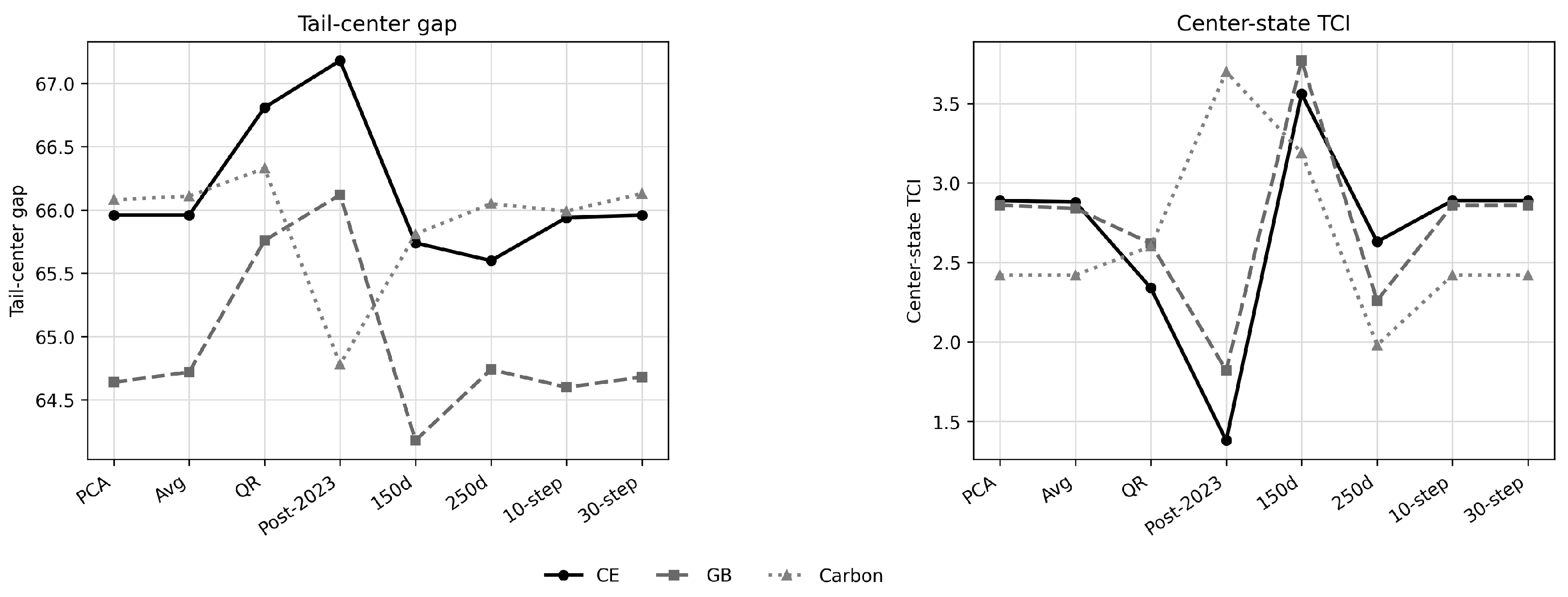
We conduct additional checks to examine whether the baseline findings depend on the PCA construction of the GSBI, the concentration of the sample around the most acute COVID-19 and initial Russia–Ukraine-war disruption periods, or the main QQC tuning choices. Table 6 reports compact robustness evidence for the GSBI pairs, while Appendix A reports the corresponding core robustness figures. First, replacing the PCA factor with a simple standardized average of the three regional SBI series yields virtually identical results. For example, the CE pair has a baseline mean TCI of 23.42 and an average-index mean TCI of 23.43; the corresponding tail–center gaps are both 65.96. Second, replacing the PCA factor with a nonlinear quantile-rank GSBI also preserves the main finding. The quantile-rank factor maps each regional SBI level into an inverse-normal empirical quantile score before aggregation, so it is less tied to linear covariance structure than PCA. Under this construction, the tail–center gaps remain 66.81 for CE, 65.76 for GB, and 66.33 for Carbon. Third, when the sample is restricted to the post-2023 period, after the most acute COVID-19 disruption and the initial Russia–Ukraine-war shock period, the tail-dominance pattern remains visible. The center TCI values remain low (1.38–3.70), while the tail–center gaps remain large (64.78–67.18). Fourth, alternative rolling windows and forecast horizons leave the main conclusion unchanged: connectedness is weak near the median state but rises sharply at joint- and cross-tail quantile combinations.
These checks support the central empirical message while also clarifying its scope. The evidence is not a claim that supply bottlenecks are the sole source of movements in green assets, nor do the checks fully control for common drivers such as broad market volatility, interest rates, energy prices, inflation news, global risk sentiment, or climate-policy news. Rather, they show that the state-dependent connectedness pattern is not sensitive to alternative GSBI construction, including a nonlinear quantile-rank aggregation, a less crisis-concentrated subsample, and reasonable changes in QQC window and horizon choices.

5. Conclusions and Discussion

This paper examines how supply chain bottleneck indicators are connected with the green finance market, represented by clean energy equities, green bonds, and carbon prices. Using the GSBI constructed by PCA together with three regional SBI indicators, and estimating pairwise quantile-on-quantile connectedness, we document a strongly nonlinear and state-dependent relationship between real-economy supply stress and green financial markets.
Three findings stand out. First, connectedness is consistently weakest around the center of the joint distribution and strongest at joint or cross-tail quantile combinations. This implies that supply bottleneck indicators matter most for green-finance connectedness when market conditions are stressed, whereas normal periods are characterized by relatively loose coupling and greater diversification potential. Second, supply bottlenecks frequently have positive net connectedness positions in extreme states, but this dominance is not uniform through time or across markets. Carbon prices, in particular, often feed connectedness back into the bilateral system, suggesting that the regulatory-pricing node of green finance is more endogenous than clean energy equities or green bonds. Third, the origin of the bottleneck matters: Chinese and U.S. bottlenecks are most tightly linked with clean energy equities, whereas euro-area bottlenecks are especially relevant for the carbon market.
These findings carry implications for investors, policymakers, and systemic-risk monitoring. For portfolio allocation, they imply that diversification across green finance submarkets is most limited precisely when supply chain stress is most severe. The practical use of the results is horizon specific. Over short horizons, from daily monitoring to roughly one trading month, risk managers can use SBI-type measures as early-warning inputs for tail-state stress tests, rapid exposure reduction, and liquidity buffers, especially for clean-energy equity positions when China or U.S. bottleneck indicators enter upper-tail states. Over medium horizons, such as one to six months, the results point to reassessing green-bond duration and liquidity exposure when bottlenecks coincide with inflation and rate-pressure news, because the financing node can shift between weaker and stronger net connectedness positions. Over longer allocation horizons, investors and climate-risk managers should treat carbon-linked exposure separately because carbon prices can become a feedback node rather than a passive hedge when regulatory expectations, energy-cost pressure, and compliance demand are repriced. For policymakers, the results suggest three practical monitoring priorities: tracking clean-energy supply bottlenecks as valuation-risk signals, monitoring green bond financing conditions when bottlenecks interact with inflation and interest-rate expectations, and incorporating carbon-market feedback into transition-risk surveillance. Climate and energy regulators should also coordinate carbon-market surveillance with supply-chain monitoring, because energy-cost shocks and regulatory expectations can jointly amplify carbon-price and bottleneck connectedness. The link to climate-risk hedging and news-based financial signals is consistent with the broader evidence that climate news and risk salience affect investor behavior and portfolio flows [51,52]. More broadly, the results show that green finance should be viewed as a complex financial segment whose resilience depends on how external disturbances are associated with internal connectedness roles and cross-market coupling.
The paper also has important limitations. The QQC framework is implemented pairwise in order to preserve transparency and state-specific granularity, but this design does not fully uncover all underlying structural channels or common drivers. The evidence should therefore be interpreted as state-dependent connectedness rather than as a structural causal estimate of supply bottlenecks on green finance. The robustness checks are sensitivity checks, not common-driver controls, and should not be interpreted as fully partialling out broad volatility, interest rates, energy prices, inflation news, global risk sentiment, or climate-policy news. The baseline GSBI is constructed using PCA, a linear dimension-reduction method; although the average-index and quantile-rank robustness checks support the main findings, future work could develop fully nonlinear factor models for global bottleneck pressure. The carbon-market proxy is based on a provider-constructed continuous EUA futures settlement-price series and does not allow us to model contract-level roll dates, roll yields, or maturity-specific futures exposure. Future work could extend the analysis to multivariate nonlinear network settings, incorporate explicit macroeconomic exogenous shock variables, or compare alternative supply-chain and carbon-market indicators. Even with these limitations, the results provide a useful step toward understanding how supply chain disruptions are associated with changes in green-finance connectedness and how system architecture changes under stress.

Author Contributions

J.Y.: Conceptualization, writing original draft, writing—review & editing, and methodology. J.W.: Supervision, investigation, and writing—review & editing. H.F.: Writing—review & editing. J.S.: Writing—review & editing, supervision, project administration, and funding acquisition. All authors have read and agreed to the published version of the manuscript.

Funding

The research is supported by National Natural Science Foundation of China (NSFC) grants No. 71988101 and No. 72173120.

Data Availability Statement

The data used in this study are compiled from publicly accessible market sources and third-party databases, but licensing restrictions apply to parts of the exchange-level trading data. The processed dataset required to reproduce the main results is available from the corresponding author upon reasonable request.

Acknowledgments

During the preparation of this manuscript, the author used Gemini 3.1 Pro for the purposes of language polishing and grammar correction. The authors have thoroughly reviewed and edited the generated output, and they take full responsibility for the content and accuracy of this publication.

Conflicts of Interest

The authors declare no conflicts of interest.

Abbreviations

The following abbreviations are used in this manuscript:
SBISupply Bottleneck Index
GSBIGlobal Supply Bottleneck Index
PCAPrincipal Component Analysis
QVARQuantile Vector Autoregression
QQCQuantile-on-Quantile Connectedness
GFEVDGeneralized Forecast Error Variance Decomposition
TCITotal Connectedness Index
CEClean Energy Equities
GBGreen Bonds
EUREuro-area aggregate SBI
EU ETSEuropean Union Emissions Trading System
EUAEuropean Union Allowance

Appendix A. Additional Robustness Evidence

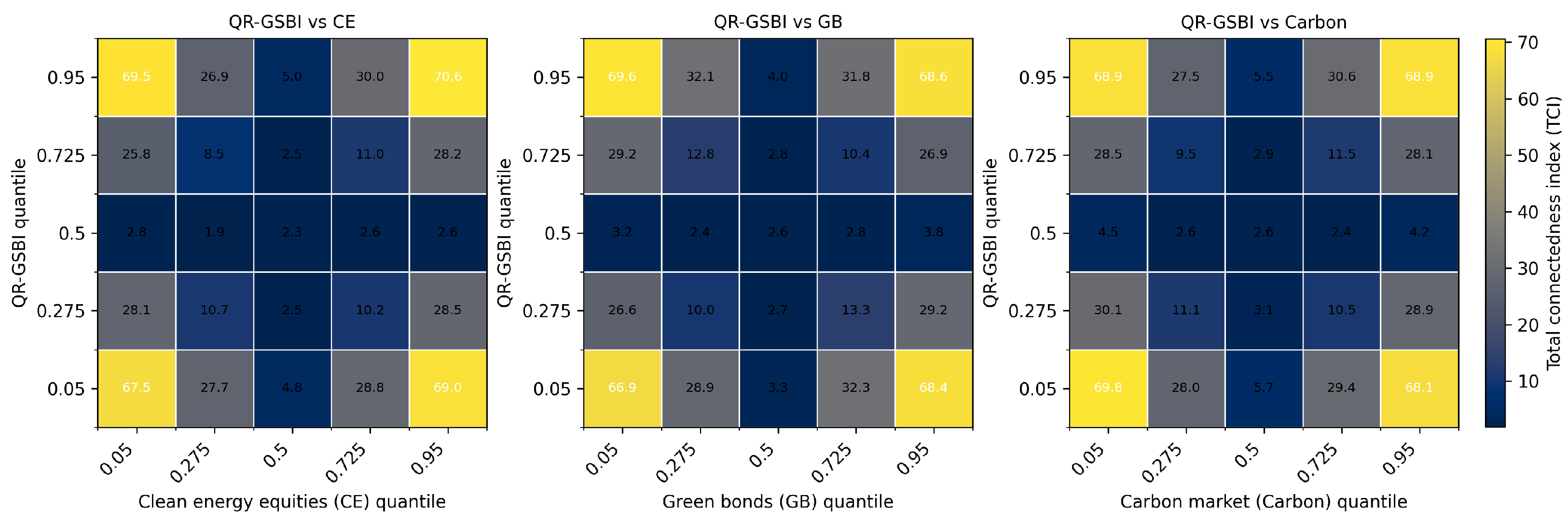
This appendix reports the main graphical evidence for the robustness checks summarized in Section 4.4. The quantile-rank GSBI (QR-GSBI) is constructed from the regional SBI level series as follows. Let R = { C H N , U S A , E U R } denote the three regions and let S B I t r be the raw level of region r at date t = 1 , , T . The empirical quantile rank of region r is
u r , t = rank ( S B I t r ) 0.5 T , r R ,
where rank ( S B I t r ) is the ascending sample rank within the region-specific level series. The rank is then mapped into an inverse-normal score,
z r , t = Φ 1 ( u r , t ) ,
where Φ 1 ( · ) denotes the inverse cumulative distribution function of the standard normal distribution. The level form of the quantile-rank GSBI is the equal-weighted average
QR-GSB I t = 1 3 r R z r , t .
Because the resulting score can take positive or negative values, the series entering the QQC system is its first difference:
Δ QR-GSB I t = QR-GSB I t QR-GSB I t 1 .
This nonlinear, rank-based aggregation gives greater relative emphasis to regional tail positions than linear standardization. The resulting transformed series has a correlation of 0.7255 with the PCA-based GSBI changes and 0.7269 with the average GSBI changes, indicating that it captures the same broad bottleneck cycle while allowing a nonlinear tail-sensitive aggregation.
Figure A1. Quantile-rank GSBI robustness: average total connectedness surfaces. Notes: QR-GSBI denotes the quantile-rank global Supply Bottleneck Index constructed from inverse-normal empirical quantile scores of the China, U.S., and euro-area SBI level series and then first-differenced before estimation. Each panel reports the average total connectedness index (TCI) surface between QR-GSBI changes and one green-finance market return. The vertical axis reports QR-GSBI quantiles, and the horizontal axis reports the corresponding clean energy equity, green bond, or carbon-market return quantiles. The heatmaps use a perceptually ordered cividis color scale, with darker cells indicating stronger total connectedness.
Systems 14 00652 g0a1
Figure A2. Core robustness diagnostics for global supply bottleneck connectedness. Notes: GSBI denotes the global Supply Bottleneck Index. The left panel compares tail–center gaps across the PCA baseline, average GSBI, quantile-rank GSBI, post-2023 subsample, alternative rolling windows, and alternative forecast horizons. The right panel reports the corresponding center-state TCI at the ( 0.50 , 0.50 ) quantile pair. Lines use distinct grayscale tones, markers, and line styles to remain distinguishable in black-and-white printing. Tail–center gaps remain high and center-state connectedness remains low across specifications.
Systems 14 00652 g0a2

Notes

1
2
3
4

References

  1. Ivanov, D. Predicting the impacts of epidemic outbreaks on global supply chains: A simulation-based analysis on the coronavirus outbreak (COVID-19/SARS-CoV-2) case. Transp. Res. Part E Logist. Transp. Rev. 2020, 136, 101922. [Google Scholar] [CrossRef]
  2. Ramani, V.; Ghosh, D.; Sodhi, M.S. Understanding systemic disruption from the COVID-19-induced semiconductor shortage for the auto industry. Omega 2022, 113, 102720. [Google Scholar] [CrossRef]
  3. Wan, Z.; Su, Y.; Li, Z.; Zhang, X.; Zhang, Q.; Chen, J. Analysis of the impact of Suez Canal blockage on the global shipping network. Ocean Coast. Manag. 2023, 245, 106868. [Google Scholar] [CrossRef]
  4. Chen, J.; Fang, Q.; Li, C.; Xu, X.; Mao, Y.; Yu, F. Impact of the Russia-Ukraine conflict on the resilience of global shipping supply chains. Reg. Stud. Mar. Sci. 2025, 91, 104502. [Google Scholar] [CrossRef]
  5. Baldwin, R.; Freeman, R. Risks and global supply chains: What we know and what we need to know. Annu. Rev. Econ. 2022, 14, 153–180. [Google Scholar] [CrossRef]
  6. Guerrieri, V.; Lorenzoni, G.; Straub, L.; Werning, I. Macroeconomic Implications of COVID-19: Can Negative Supply Shocks Cause Demand Shortages? Am. Econ. Rev. 2022, 112, 1437–1474. [Google Scholar] [CrossRef]
  7. Liu, Z.; Nguyen, T.L. Global supply chain pressures and US inflation. FRBSF Econ. Lett. 2023, 14, 1–6. [Google Scholar]
  8. Gordon, M.V.; Clark, T.E. The impacts of supply chain disruptions on inflation. Econ. Comment. 2023, 1–8. [Google Scholar] [CrossRef]
  9. Kemp, H.; Portillo, M.R.A.; Portillo, R.; Santoro, M. Assessing the Impact of Supply Disruptions on the Global Pandemic Recovery; Technical Report; International Monetary Fund: Washington, DC, USA, 2023. [Google Scholar]
  10. Diaz, E.M.; Cuñado, J.; de Gracia, F.P. Global drivers of inflation: The role of supply chain disruptions and commodity price shocks. Econ. Model. 2024, 140, 106860. [Google Scholar] [CrossRef]
  11. Ascari, G.; Bonam, D.; Smadu, A. Global supply chain pressures, inflation, and implications for monetary policy. J. Int. Money Financ. 2024, 142, 103029. [Google Scholar] [CrossRef]
  12. Burriel, P.; Kataryniuk, I.; Moreno Pérez, C.; Viani, F. A new supply bottlenecks index based on newspaper data. Int. J. Cent. Bank. 2023. [Google Scholar] [CrossRef]
  13. Taghizadeh-Hesary, F.; Yoshino, N. The way to induce private participation in green finance and investment. Financ. Res. Lett. 2019, 31, 98–103. [Google Scholar] [CrossRef]
  14. Fu, C.; Lu, L.; Pirabi, M. Advancing green finance: A review of climate change and decarbonization. Digit. Econ. Sustain. Dev. 2024, 2, 1. [Google Scholar] [CrossRef]
  15. Bolton, P.; Kacperczyk, M. Global Pricing of Carbon-Transition Risk. J. Financ. 2023, 78, 3677–3754. [Google Scholar] [CrossRef]
  16. Pástor, Ľ.; Stambaugh, R.F.; Taylor, L.A. Sustainable investing in equilibrium. J. Financ. Econ. 2021, 142, 550–571. [Google Scholar] [CrossRef]
  17. Reboredo, J.C. Green bond and financial markets: Co-movement, diversification and price spillover effects. Energy Econ. 2018, 74, 38–50. [Google Scholar] [CrossRef]
  18. Reboredo, J.C.; Ugolini, A. Price connectedness between green bond and financial markets. Econ. Model. 2020, 88, 25–38. [Google Scholar] [CrossRef]
  19. Reboredo, J.C.; Ugolini, A.; Aiube, F.A.L. Network connectedness of green bonds and asset classes. Energy Econ. 2020, 86, 104629. [Google Scholar] [CrossRef]
  20. Liu, N.; Liu, C.; Da, B.; Zhang, T.; Guan, F. Dependence and risk spillovers between green bonds and clean energy markets. J. Clean. Prod. 2021, 279, 123595. [Google Scholar] [CrossRef]
  21. Pham, L. Frequency connectedness and cross-quantile dependence between green bond and green equity markets. Energy Econ. 2021, 98, 105257. [Google Scholar] [CrossRef]
  22. Naeem, M.A.; Nguyen, T.T.H.; Nepal, R.; Ngo, Q.T.; Taghizadeh-Hesary, F. Asymmetric relationship between green bonds and commodities: Evidence from extreme quantile dependence. Financ. Res. Lett. 2021, 43, 101983. [Google Scholar] [CrossRef]
  23. Tiwari, A.K.; Abakah, E.J.A.; Gabauer, D.; Dwumfour, R.A. Dynamic spillover effects among green bond, renewable energy stocks and carbon markets during COVID-19 pandemic: Implications for hedging and investments strategies. Glob. Financ. J. 2022, 51, 100692. [Google Scholar] [CrossRef] [PubMed]
  24. Long, S.; Tian, H.; Li, Z. Dynamic spillovers between uncertainties and green bond markets in the US, Europe, and China: Evidence from the quantile VAR framework. Int. Rev. Financ. Anal. 2022, 84, 102416. [Google Scholar] [CrossRef]
  25. Chatziantoniou, I.; Abakah, E.J.A.; Gabauer, D.; Tiwari, A.K. Quantile time–frequency price connectedness between green bond, green equity, sustainable investments and clean energy markets. J. Clean. Prod. 2022, 361, 132088. [Google Scholar] [CrossRef]
  26. Ringstad, I.E.F.; Tselika, K. Connectedness between green bonds, clean energy markets and carbon quota prices: Time and frequency dynamics. J. Commod. Mark. 2024, 36, 100442. [Google Scholar] [CrossRef]
  27. Wang, Y.; Zhao, X.; Shang, J. Dynamic risk spillover in green financial markets: A wavelet frequency analysis from China. Energy Econ. 2025, 143, 108301. [Google Scholar] [CrossRef]
  28. Huang, Z.; Ding, X.; Wang, Y. Risk spillover and network connectedness analysis of green financial and related financial markets: Evidence from China. Humanit. Soc. Sci. Commun. 2026, 13, 344. [Google Scholar] [CrossRef]
  29. Barrot, J.N.; Sauvagnat, J. Input specificity and the propagation of idiosyncratic shocks in production networks. Q. J. Econ. 2016, 131, 1543–1592. [Google Scholar] [CrossRef]
  30. Carvalho, V.M.; Nirei, M.; Saito, Y.U.; Tahbaz-Salehi, A. Supply Chain Disruptions: Evidence from the Great East Japan Earthquake. Q. J. Econ. 2021, 136, 1255–1321. [Google Scholar] [CrossRef]
  31. Gilchrist, S.; Zakrajšek, E. Credit Spreads and Business Cycle Fluctuations. Am. Econ. Rev. 2012, 102, 1692–1720. [Google Scholar] [CrossRef]
  32. Youssef, M.; Gallas, S.; Urom, C. Cryptocurrency price dynamics during supply chain disruptions: A quantile-on-quantile connectedness approach. Financ. Res. Lett. 2026, 93, 109600. [Google Scholar] [CrossRef]
  33. Gabauer, D.; Stenfors, A. Quantile-on-quantile connectedness measures: Evidence from the US treasury yield curve. Financ. Res. Lett. 2024, 60, 104852. [Google Scholar] [CrossRef]
  34. Mizgier, K.J.; Jüttner, M.P.; Wagner, S.M. Bottleneck identification in supply chain networks. Int. J. Prod. Res. 2013, 51, 1477–1490. [Google Scholar] [CrossRef]
  35. Xu, D.; Zhang, Y.; Li, Y.; Wang, X.; Yang, Z. Path analysis for carbon transfers embodied in China’s international trade and policy implications for mitigation targets. J. Clean. Prod. 2022, 334, 130207. [Google Scholar] [CrossRef]
  36. Ehlers, T.; Packer, F. Green bond finance and certification. BIS Q. Rev. 2017. Available online: https://www.bis.org/publ/qtrpdf/r_qt1709h.htm (accessed on 1 May 2026).
  37. Flammer, C. Corporate green bonds. J. Financ. Econ. 2021, 142, 499–516. [Google Scholar] [CrossRef]
  38. Koch, N.; Fuss, S.; Grosjean, G.; Edenhofer, O. Causes of the EU ETS price drop: Recession, CDM, renewable policies or a bit of everything?—New evidence. Energy Policy 2014, 73, 676–685. [Google Scholar] [CrossRef]
  39. Chevallier, J. Carbon futures and macroeconomic risk factors: A view from the EU ETS. Energy Econ. 2009, 31, 614–625. [Google Scholar] [CrossRef]
  40. Hammoudeh, S.; Ajmi, A.N.; Mokni, K. Relationship between green bonds and financial and environmental variables: A novel time-varying causality. Energy Econ. 2020, 92, 104941. [Google Scholar] [CrossRef]
  41. Chatziantoniou, I.; Gabauer, D.; Stenfors, A. Interest rate swaps and the transmission mechanism of monetary policy: A quantile connectedness approach. Econ. Lett. 2021, 204, 109891. [Google Scholar] [CrossRef]
  42. Ando, T.; Greenwood-Nimmo, M.; Shin, Y. Quantile connectedness: Modeling tail behavior in the topology of financial networks. Manag. Sci. 2022, 68, 2401–2431. [Google Scholar] [CrossRef]
  43. Diebold, F.X.; Yilmaz, K. Better to give than to receive: Predictive directional measurement of volatility spillovers. Int. J. Forecast. 2012, 28, 57–66. [Google Scholar] [CrossRef]
  44. Bai, Y.; Okullo, S.J. Drivers and pass-through of the EU ETS price: Evidence from the power sector. Energy Econ. 2023, 123, 106698. [Google Scholar] [CrossRef]
  45. Sitarz, J.; Pahle, M.; Osorio, S.; Luderer, G.; Pietzcker, R. EU carbon prices signal high policy credibility and farsighted actors. Nat. Energy 2024, 9, 691–702. [Google Scholar] [CrossRef]
  46. European Commission. Trends in Carbon Intensity and the Macroeconomic Role of the EU Emissions Trading System. 2026. Available online: https://economy-finance.ec.europa.eu/trends-carbon-intensity-and-macroeconomic-role-eu-emissions-trading-system_en (accessed on 1 May 2026).
  47. International Energy Agency. Solar PV Global Supply Chains. 2022. Available online: https://www.iea.org/reports/solar-pv-global-supply-chains (accessed on 1 May 2026).
  48. International Energy Agency. Global EV Outlook 2025: Electric Vehicle Batteries. 2025. Available online: https://www.iea.org/reports/global-ev-outlook-2025/electric-vehicle-batteries (accessed on 1 May 2026).
  49. International Energy Agency. World Energy Investment 2024: United States. 2024. Available online: https://www.iea.org/reports/world-energy-investment-2024/united-states (accessed on 1 May 2026).
  50. International Carbon Action Partnership. EU Emissions Trading System (EU ETS). 2026. Available online: https://icapcarbonaction.com/en/ets/eu-emissions-trading-system-eu-ets (accessed on 1 May 2026).
  51. Engle, R.F.; Giglio, S.; Kelly, B.; Lee, H.; Stroebel, J. Hedging climate change news. Rev. Financ. Stud. 2020, 33, 1184–1216. [Google Scholar] [CrossRef]
  52. Mugerman, Y.; Steinberg, N.; Wiener, Z. The exclamation mark of Cain: Risk salience and mutual fund flows. J. Bank. Financ. 2022, 134, 106332. [Google Scholar] [CrossRef]
Figure 1. Time-series plots of transformed supply chain bottleneck changes. Notes: GSBI denotes transformed changes in the global Supply Bottleneck Index obtained from principal component analysis (PCA); CHN SBI, USA SBI, and EUR SBI denote transformed changes in the regional Supply Bottleneck Index (SBI) series for China, the United States, and the euro area, respectively. The regional SBI variables are log changes of positive newspaper-based pressure indices, while the PCA-based GSBI is first-differenced because the standardized factor can take positive or negative values. The plots highlight pronounced bursts of volatility around major global stress episodes.
Systems 14 00652 g001
Figure 2. Time-series plots of transformed green finance returns. Notes: CE, GB, and Carbon denote the return series of the S&P Clean Energy Index, the S&P Dow Jones Green Bond Index, and ICE EUA futures, respectively. Carbon exhibits the largest and most persistent volatility bursts, while green bonds remain comparatively stable.
Systems 14 00652 g002
Figure 3. Pearson correlation matrix of supply bottleneck changes and green finance returns. Notes: The lower triangle reports pairwise scatterplots, the upper triangle reports Pearson correlation coefficients, and the diagonal shows the marginal distributions. GSBI denotes transformed changes in the global Supply Bottleneck Index; CHN SBI, USA SBI, and EUR SBI denote transformed regional Supply Bottleneck Index changes. CE, GB, and Carbon denote clean energy, green bond, and carbon market returns, respectively. *** p < 0.01 .
Systems 14 00652 g003
Figure 4. Principal component analysis of regional supply bottleneck indices. Notes: The left panel reports the loading plot for the standardized regional Supply Bottleneck Index (SBI) level series, while the right panel shows the scree plot of the corresponding eigenvalues. The positive and closely aligned loadings of CHN SBI, USA SBI, and EUR SBI on the first dimension indicate that the three regional level series share a strong common factor. The scree plot and Table 4 show that the first principal component explains 86.17% of the total variance, which supports using PC1 as the empirical proxy for the global Supply Bottleneck Index (GSBI). The sign of PC1 is normalized to comove positively with the regional average, and the resulting factor is first-differenced before QQC estimation.
Systems 14 00652 g004
Figure 5. Average total and net dynamic quantile-on-quantile connectedness between GSBI and green finance markets. (a1) GSBI ↔ CE; (a2) Net GSBI ↔ CE; (b1) GSBI ↔ GB; (b2) Net GSBI ↔ GB; (c1) GSBI ↔ Carbon; (c2) Net GSBI ↔ Carbon. Notes: GSBI denotes the global Supply Bottleneck Index. Panels in the left column report the average total connectedness index (TCI), while panels in the right column report the average net connectedness (NET). Positive NET values indicate that the GSBI has the stronger net connectedness position relative to the corresponding green finance market; negative values indicate that the green finance market has the stronger net connectedness position relative to the GSBI. The vertical axes represent the quantiles of GSBI changes and the horizontal axes represent the quantiles of green finance market returns, using the five-point grid { 0.05 , 0.275 , 0.50 , 0.725 , 0.95 } . CE, GB, and Carbon denote clean energy equities, green bonds, and the carbon market, respectively. All estimations employ a 200-day rolling-window QVAR( τ 1 , τ 2 ) framework with a BIC-selected lag order of 1 and a 20-step-ahead forecast horizon.
Systems 14 00652 g005
Figure 6. Dynamic diagonal- and anti-diagonal-state total connectedness between GSBI and green finance markets. (a) Dynamic diagonal- and anti-diagonal-state total connectedness: GSBI ↔ CE. (b) Dynamic diagonal- and anti-diagonal-state total connectedness: GSBI ↔ GB. (c) Dynamic diagonal- and anti-diagonal-state total connectedness: GSBI ↔ Carbon. Notes: GSBI denotes the global Supply Bottleneck Index. Each panel reports the time-varying diagonal-state and anti-diagonal-state total connectedness, together with their difference ( Δ T C I ), between GSBI changes and the corresponding green finance market return. The green line denotes diagonal-state TCI, computed from same-state quantile pairs, while the red line denotes anti-diagonal-state TCI, computed from opposite-tail quantile pairs. The blue line ( Δ T C I ) reports diagonal-state TCI minus anti-diagonal-state TCI. Positive Δ T C I values indicate stronger same-state connectedness; negative values indicate stronger opposite-tail connectedness. CE, GB, and Carbon refer to clean energy, green bond, and carbon markets, respectively.
Systems 14 00652 g006
Figure 7. Average total and net dynamic quantile-on-quantile connectedness between China SBI and green finance markets. (a1) CHN SBI ↔ CE; (a2) Net CHN SBI ↔ CE; (b1) CHN SBI ↔ GB; (b2) Net CHN SBI ↔ GB; (c1) CHN SBI ↔ Carbon; (c2) Net CHN SBI ↔ Carbon. Notes: SBI denotes the Supply Bottleneck Index. Panels in the left column report the average total connectedness index (TCI), while panels in the right column report the average net connectedness (NET). Positive NET values indicate that the SBI has the stronger net connectedness position relative to the corresponding green finance market; negative values indicate that the green finance market has the stronger net connectedness position relative to the SBI. The vertical axes represent the quantiles of SBI changes and the horizontal axes represent the quantiles of green finance market returns, using the five-point grid { 0.05 , 0.275 , 0.50 , 0.725 , 0.95 } . CE, GB, and Carbon denote clean energy equities, green bonds, and the carbon market, respectively. All estimations employ a 200-day rolling-window QVAR( τ 1 , τ 2 ) framework with a BIC-selected lag order of 1 and a 20-step-ahead forecast horizon.
Systems 14 00652 g007
Figure 8. Dynamic diagonal- and anti-diagonal-state total connectedness between China SBI and green finance markets. (a) Dynamic diagonal- and anti-diagonal-state total connectedness: CHN SBI ↔ CE. (b) Dynamic diagonal- and anti-diagonal-state total connectedness: CHN SBI ↔ GB. (c) Dynamic diagonal- and anti-diagonal-state total connectedness: CHN SBI ↔ Carbon. Notes: SBI denotes the Supply Bottleneck Index. Each panel reports the time-varying diagonal-state and anti-diagonal-state total connectedness, together with their difference ( Δ T C I ), between China SBI and the corresponding green finance market. The green line denotes diagonal-state TCI, computed from same-state quantile pairs, while the red line denotes anti-diagonal-state TCI, computed from opposite-tail quantile pairs. The blue line ( Δ T C I ) reports diagonal-state TCI minus anti-diagonal-state TCI. Positive Δ T C I values indicate stronger same-state connectedness; negative values indicate stronger opposite-tail connectedness. CE, GB, and Carbon refer to clean energy, green bond, and carbon markets, respectively.
Systems 14 00652 g008
Figure 9. Average total and net dynamic quantile-on-quantile connectedness between USA SBI and green finance markets. (a1) USA SBI ↔ CE; (a2) Net USA SBI ↔ CE; (b1) USA SBI ↔ GB; (b2) Net USA SBI ↔ GB; (c1) USA SBI ↔ Carbon; (c2) Net USA SBI ↔ Carbon. Notes: SBI denotes the Supply Bottleneck Index. Panels in the left column report the average total connectedness index (TCI), while panels in the right column report the average net connectedness (NET). Positive NET values indicate that the SBI has the stronger net connectedness position relative to the corresponding green finance market; negative values indicate that the green finance market has the stronger net connectedness position relative to the SBI. The vertical axes represent the quantiles of SBI changes and the horizontal axes represent the quantiles of green finance market returns, using the five-point grid { 0.05 , 0.275 , 0.50 , 0.725 , 0.95 } . CE, GB, and Carbon denote clean energy equities, green bonds, and the carbon market, respectively. All estimations employ a 200-day rolling-window QVAR( τ 1 , τ 2 ) framework with a BIC-selected lag order of 1 and a 20-step-ahead forecast horizon.
Systems 14 00652 g009
Figure 10. Dynamic diagonal- and anti-diagonal-state total connectedness between USA SBI and green finance markets. (a) Dynamic diagonal- and anti-diagonal-state total connectedness: USA SBI ↔ CE. (b) Dynamic diagonal- and anti-diagonal-state total connectedness: USA SBI ↔ GB. (c) Dynamic diagonal- and anti-diagonal-state total connectedness: USA SBI ↔ Carbon. Notes: SBI denotes the Supply Bottleneck Index. Each panel reports the time-varying diagonal-state and anti-diagonal-state total connectedness, together with their difference ( Δ T C I ), between USA SBI and the corresponding green finance market. The green line denotes diagonal-state TCI, computed from same-state quantile pairs, while the red line denotes anti-diagonal-state TCI, computed from opposite-tail quantile pairs. The blue line ( Δ T C I ) reports diagonal-state TCI minus anti-diagonal-state TCI. Positive Δ T C I values indicate stronger same-state connectedness; negative values indicate stronger opposite-tail connectedness. CE, GB, and Carbon refer to clean energy, green bond, and carbon markets, respectively.
Systems 14 00652 g010
Figure 11. Average total and net dynamic quantile-on-quantile connectedness between Eurozone SBI and green finance markets. (a1) EUR SBI ↔ CE; (a2) Net EUR SBI ↔ CE; (b1) EUR SBI ↔ GB; (b2) Net EUR SBI ↔ GB; (c1) EUR SBI ↔ Carbon; (c2) Net EUR SBI ↔ Carbon. Notes: SBI denotes the Supply Bottleneck Index. Panels in the left column report the average total connectedness index (TCI), while panels in the right column report the average net connectedness (NET). Positive NET values indicate that the SBI has the stronger net connectedness position relative to the corresponding green finance market; negative values indicate that the green finance market has the stronger net connectedness position relative to the SBI. The vertical axes represent the quantiles of SBI changes and the horizontal axes represent the quantiles of green finance market returns, using the five-point grid { 0.05 , 0.275 , 0.50 , 0.725 , 0.95 } . CE, GB, and Carbon denote clean energy equities, green bonds, and the carbon market, respectively. All estimations employ a 200-day rolling-window QVAR( τ 1 , τ 2 ) framework with a BIC-selected lag order of 1 and a 20-step-ahead forecast horizon.
Systems 14 00652 g011
Figure 12. Dynamic diagonal- and anti-diagonal-state total connectedness between Eurozone SBI and green finance markets. (a) Dynamic diagonal- and anti-diagonal-state total connectedness: EUR SBI ↔ CE. (b) Dynamic diagonal- and anti-diagonal-state total connectedness: EUR SBI ↔ GB. (c) Dynamic diagonal- and anti-diagonal-state total connectedness: EUR SBI ↔ Carbon. Notes: SBI denotes the Supply Bottleneck Index. Each panel reports the time-varying diagonal-state and anti-diagonal-state total connectedness, together with their difference ( Δ T C I ), between EUR SBI and the corresponding green finance market. The green line denotes diagonal-state TCI, computed from same-state quantile pairs, while the red line denotes anti-diagonal-state TCI, computed from opposite-tail quantile pairs. The blue line ( Δ T C I ) reports diagonal-state TCI minus anti-diagonal-state TCI. Positive Δ T C I values indicate stronger same-state connectedness; negative values indicate stronger opposite-tail connectedness. CE, GB, and Carbon refer to clean energy, green bond, and carbon markets, respectively.
Systems 14 00652 g012
Table 1. Summary of closely related studies.
MarketAnalysis Features
Study Period Method SC CE GB Carbon Tail Regional Ext.
Youssef et al. (2026) [32]2017–2024QQC×××
Ringstad & Tselika (2024) [26]2014–2022DY/BK××××
Wang et al. (2025) [27]2015–2023Wavelet××××
Huang et al. (2026) [28]2015–2023Network××××
Chatziantoniou et al. (2022) [25]2014–2021QVAR××××
Tiwari et al. (2022) [23]2012–2021TVP-VAR××××
Long et al. (2022) [24]2014–2021QVAR××××
Naeem et al. (2021) [22]2014–2020Copula×××××
Pham (2021) [21]2014–2020QVAR + Freq××××
Liu et al. (2021) [20]2010–2019Copula×××××
Reboredo (2018) [17]2013–2018VAR/Cop××××××
Burriel et al. (2023) [12]2003–2022NLP/Text××××
This paper2018–2026QQC
Notes: SC = supply chain bottleneck variable included; CE = clean energy equities; GB = green bonds; Tail = explicit tail/extreme-state analysis; Regional = comparison of regional indicators or markets; Ext. = real-economy external shock (non-financial driver). Method abbreviations: QQC = quantile-on-quantile connectedness; DY/BK = Diebold–Yilmaz/Baruník–Křehlík time-frequency connectedness; TVP-VAR = time-varying parameter VAR connectedness; QVAR = quantile VAR connectedness; Cop = copula; QVAR + Freq = frequency connectedness with quantile VAR connectedness; NLP = newspaper-based text analysis. ✓ = yes; × = no.
Table 2. Descriptive statistics.
GSBICHN SBIUSA SBIEUR SBI
Mean0.00130.00050.00070.0010
Median−0.001−0.0024−0.00110.001
Min−0.9506−0.3513−0.4284−1.1846
Max0.74830.44140.43330.6982
Std. Dev0.10160.07320.07690.0977
Skewness0.11710.31270.1588−0.8381
Kurtosis10.51575.37776.429316.2553
JB4994.4816 ***533.9322 ***1047.7149 ***15,768.6313 ***
ADF−32.28 ***−36.9402 ***−40.335 ***−42.2544 ***
PP−34.7402 ***−37.5891 ***−41.3146 ***−42.7624 ***
CEGBCarbon
Mean0.00030.00010.0011
Median0.00030.00020.001
Min−0.125−0.0156−0.1942
Max0.11030.0120.1614
Std. Dev0.01620.00230.0268
Skewness−0.3537−0.4183−0.4975
Kurtosis9.83567.74427.9747
JB4171.6525 ***2049.9674 ***2273.5178 ***
ADF−41.9415 ***−38.0582 ***−47.4972 ***
PP−42.031 ***−38.5739 ***−47.4422 ***
Notes: GSBI denotes the global Supply Bottleneck Index constructed from principal component analysis; CHN SBI, USA SBI, and EUR SBI denote the regional Supply Bottleneck Indices for China, the United States, and the euro area, respectively. CE, GB, and Carbon denote clean energy equities, green bonds, and the carbon market (proxied by ICE EUA futures), respectively. Std. Dev. represents the standard deviation. JB, ADF, and PP denote the Jarque–Bera, Augmented Dickey–Fuller, and Phillips–Perron test statistics, respectively. *** p < 0.01.
Table 3. Statistical comparison of raw and transformed supply bottleneck indicators.
PanelSeriesNMeanMedianStd. Dev.MinMaxSkewnessKurtosisADFPP
Raw SBI levelsPCA-based GSBI level21210.006−0.5761.608−1.8785.5851.2433.707 2.740 *−2.533
CHN SBI level2121177.412134.226121.19328.622708.0371.7305.930 3.557 *** 3.499 ***
USA SBI level2121278.518200.663230.62629.5691443.9211.6235.721 3.447 *** 3.200 **
EUR SBI level2121285.689203.952234.46712.7141174.3591.1463.466 2.844 * 2.952 **
Transformed SBI changes Δ PCA-based GSBI21200.001−0.0010.102−0.9510.7480.11710.536 10.274 *** 35.392 ***
Δ log (CHN SBI)21200.000−0.0020.073−0.3510.4410.3135.386 17.802 *** 36.327 ***
Δ log (USA SBI)21200.001−0.0010.077−0.4280.4330.1596.440 16.555 *** 40.192 ***
Δ log (EUR SBI)21200.0010.0010.098−1.1850.698−0.83916.289 19.236 *** 42.204 ***
Notes: The raw level panel reports the PCA-based global Supply Bottleneck Index (GSBI) and the regional Supply Bottleneck Index (SBI) levels. The transformed panel reports the first difference of the PCA-based GSBI and the log changes of the positive regional SBI levels. ADF and PP denote the Augmented Dickey–Fuller and Phillips–Perron unit-root test statistics, respectively, both with an intercept. * p < 0.10, ** p < 0.05, *** p < 0.01.
Table 4. Importance of components in principal component analysis (PCA).
ComponentEigenvalueExplained Variance (%)Cumulative Variance (%)
PC12.585286.1786.17
PC20.27939.3195.48
PC30.13554.52100.00
Table 5. Summary of baseline quantile-on-quantile connectedness patterns.
IndicatorMarketMean TCICenter TCIJoint-Tail TCICross-Tail TCITail–Center Gap
GSBICE23.422.8967.2370.4565.96
GSBIGB23.302.8666.0069.0164.64
GSBICarbon22.772.4268.4368.5766.08
CHN SBICE22.892.2367.9368.9766.22
CHN SBIGB23.062.1767.2867.9965.46
CHN SBICarbon23.242.4569.2968.2666.32
USA SBICE22.122.0269.3269.2067.24
USA SBIGB23.042.4267.2069.1465.76
USA SBICarbon22.782.6768.6568.9766.14
EUR SBICE21.731.8668.9968.0166.64
EUR SBIGB22.892.0668.1569.5266.78
EUR SBICarbon22.021.1070.1068.7068.30
Notes: Center TCI reports the ( 0.50 , 0.50 ) quantile pair. Joint-tail TCI averages the lower–lower and upper–upper quantile pairs, and cross-tail TCI averages the lower–upper and upper–lower quantile pairs. The tail–center gap is the average of the four corner TCI values minus the center TCI.
Table 6. Robustness checks for global supply bottleneck connectedness.
SpecificationMarketMean TCICenter TCIJoint-Tail TCICross-Tail TCITail–Center Gap
BaselineCE23.422.8967.2370.4565.96
BaselineGB23.302.8666.0069.0164.64
BaselineCarbon22.772.4268.4368.5766.08
Average GSBICE23.432.8867.2170.4765.96
Average GSBIGB23.332.8466.0169.1064.72
Average GSBICarbon22.782.4268.4968.5766.11
Quantile-rank GSBICE22.732.3469.0669.2466.81
Quantile-rank GSBIGB23.382.6267.7569.0065.76
Quantile-rank GSBICarbon23.312.6069.3768.5066.33
Post-2023 subsampleCE22.831.3867.1869.9567.18
Post-2023 subsampleGB22.991.8266.2669.6266.12
Post-2023 subsampleCarbon24.093.7069.1367.8364.78
150-day windowCE24.303.5668.0170.6065.74
150-day windowGB24.443.7766.4769.4364.18
150-day windowCarbon23.823.1968.8469.1565.81
250-day windowCE22.812.6366.4470.0365.60
250-day windowGB22.552.2665.3068.7064.74
250-day windowCarbon22.151.9868.0268.0466.05
10-step horizonCE23.392.8967.2270.4365.94
10-step horizonGB23.262.8665.9568.9764.60
10-step horizonCarbon22.732.4268.3268.4965.99
30-step horizonCE23.432.8967.2470.4565.96
30-step horizonGB23.342.8666.0169.0764.68
30-step horizonCarbon22.802.4268.4868.6166.13
Notes: GSBI denotes the global Supply Bottleneck Index. The post-2023 subsample covers 3 January 2023 to 31 March 2026. Baseline settings use a 200-day rolling window, a 20-step-ahead forecast horizon, one QVAR lag, and quantiles { 0.05 , 0.275 , 0.50 , 0.725 , 0.95 } . The quantile-rank GSBI is constructed by averaging inverse-normal empirical quantile scores of the three regional SBI levels and then taking first differences.
Disclaimer/Publisher’s Note: The statements, opinions and data contained in all publications are solely those of the individual author(s) and contributor(s) and not of MDPI and/or the editor(s). MDPI and/or the editor(s) disclaim responsibility for any injury to people or property resulting from any ideas, methods, instructions or products referred to in the content.