Outlier-Driven Network Inference of Financial Time Series

Abstract

Outliers in financial time series can reveal latent inter-asset relationships that are often missed by traditional dependence measures and average dynamic models. To address this gap, we propose Outlier-Driven Network Inference (ODNI), a framework for reconstructing directed lagged Tail Outlier-Triggering Networks from financial time series. ODNI first converts multivariate return series into upper and lower tail outlier indicators using empirical quantiles, then applies a bivariate EM-based attribution model to infer lagged triggering relationships across tail channels, and finally constructs a directed weighted network by combining baseline-corrected excess activation with EM attribution weights. For controlled evaluation, we simulate multivariate time series with volatility clustering and cross-variable spillovers from a known directed interaction template using a cross-GARCH(1,1) model. Across extensive experiments, ODNI achieves the best reconstruction performance among CoVaR, a Clayton copula tail-dependent network, and DCC-GARCH, with especially strong precision. Robustness tests show stable behavior across regimes, with systematic improvement as sample length increases and true coupling becomes more identifiable. Applications to major foreign exchange rates and global stock indices further reveal clear regional structure and asymmetric sender–receiver roles across tail-triggering channels. ODNI provides a practical tool for uncovering latent risk transmission pathways driven by tail outliers.

1. Introduction

In many complex systems (e.g., financial, social, and neural systems), the underlying network structure is often hidden or only partially observable [1,2,3]. For instance, in financial markets, the true relationships among market entities are typically not directly observable. Nevertheless, these structures play a crucial role in the propagation of risk and the emergence of systemic vulnerabilities [4,5,6,7,8]. In particular, dense interconnections among financial institutions lead significantly to the development of systemic risk scenarios [9,10,11]. Furthermore, historical evidence has repeatedly demonstrated the fragility of financial markets, as illustrated by events such as the 2008 Global Financial Crisis, the 2011 European Debt Crisis, the 2015 Chinese Stock Market Crash, and the activation of circuit breakers in the stock market during the COVID-19 pandemic in 2020 [12,13,14,15].

Time series data generated by complex systems provide an important basis for inferring latent relationships among system components [16,17]. In this regard, reconstructing association networks from observational data [3,18] allows the discovery of latent relationships, offers a clearer representation of the system’s overall relational structure, and facilitates the precise identification of risk transmission pathways and contagion mechanisms [19]; the core challenge of network reconstruction is the accurate inference of “edges,” representing potential influence relationships between system entities based on time series data [20]. This task is complicated by the nonlinear, asymmetric, and time-lagged contagion mechanisms that often characterize financial markets [21,22]. Inferring hidden networks from partially observed or aggregated signals [3,19,23] is further hindered by outlier-driven volatility and heavy-tailed distributions.

As a result, identifying these latent edges becomes a complex inference problem that requires breakthroughs at the intersection of statistics, econometrics, and network science [24,25]. Traditional econometric models, such as Vector Autoregressive (VAR) models [26,27,28], often reconstruct financial networks by examining lagged interactions among time series, where model coefficients indicate directed links between assets. However, VAR and Forecast Error Variance Decomposition (FEVD) primarily capture average market dynamics and require stationary time series [29,30]. Moreover, preprocessing to address non-stationarity or outliers often eliminates critical tail risk signals. Given that financial returns frequently exhibit heavy tails, abrupt jumps, and non-Gaussian characteristics [31,32], these methods may be limited in identifying directional lagged propagation in the tails.

In this respect, copula-based methods [33,34] attempt to model nonlinear and tail dependencies, inferring stronger connections when assets co-move in the tails [35]. However, their performance is sensitive to the choice of marginal distributions [36], and they struggle with time-dependent structures [37]. Tail-oriented systemic risk measures such as CoVaR further highlight the importance of conditional risk transmission under distress states [38]. GARCH family models capture volatility clustering and allow time-varying dependence structures. For example, DCC-GARCH models time-varying conditional correlations, while multivariate GARCH frameworks have been used to study return and volatility transmission in financial markets [39]. However, dependence measures derived from second-moment dynamics are often symmetric and may not directly reveal directional lagged propagation across tail outliers. 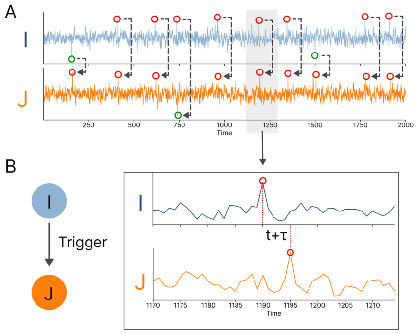As an illustrative example, Figure 1A presents the minute-by-minute price curves of an energy stock and a financial stock. Despite the apparent similarity in their trends, traditional methods indicate a weak linear correlation, low FEVD explanatory power, and only mild time-varying conditional dependence under a DCC-GARCH model. These findings suggest that there is no significant association between the two stocks during the observation period under conventional econometric frameworks.

A different picture emerges when attention is restricted to tail outliers, as illustrated in Figure 1. When the full return series $I$ and $J$ are considered, their overall relationship appears weak: the contemporaneous and lagged correlations are close to zero, and the Granger causality test does not indicate a clear predictive relationship. From the perspective of conventional average-based analysis, the two series therefore seem to have no obvious directional dependence. However, when the analysis focuses on tail outliers, a repeated lagged pattern becomes visible. Specifically, after a tail outlier occurs in series $I$ at time $t$, a tail outlier in series $J$ is frequently observed at the lagged time $t+\tau$. Although a single tail outlier is a low-probability event, the repeated occurrence of such ordered outlier-to-outlier pairs over the sample makes it a “high-probability event within low-probability events.” This pattern suggests that the relationship between the two series is not captured by ordinary correlation or Granger causality. In this statistical sense, the outliers in $I$ can be regarded as triggering outliers in $J$.

This observation motivates the Tail Outlier-Triggering Network studied in this paper. The network captures repeated lagged patterns in which a tail outlier in one asset is followed by an increased probability of a tail outlier in another asset. A directed link from asset $i$ to asset $j$ represents a statistical tail outlier relationship, in which a tail outlier in $i$ at time $t$ is followed by an increased probability of a tail outlier in $j$ at time $t+\tau$, with its strength estimated after accounting for the target-specific spontaneous activation baseline.

Against this background, understanding how tail outliers occur in an ordered manner across assets becomes critically important. When the true network structure is unobservable, identifying abnormal transmission pathways provides useful information for systemic risk monitoring [40,41]. In this context, statistical inference methods, grounded in rigorous mathematical theory, demonstrate robust performance by generating probability distributions over reconstructed network ensembles [42,43,44]. In particular, bivariate statistical inference with an EM attribution mechanism provides a probabilistic way to infer pairwise triggering relationships from binary sequences [42]. As a result, this article develops Outlier-Driven Network Inference (ODNI) for reconstructing directed lagged Tail Outlier-Triggering Networks from financial time series. ODNI first converts each return series into upper and lower tail outlier indicators using empirical quantiles. This transformation turns continuous returns into tail event activation sequences and allows the model to focus on the occurrence, sign, and timing of extreme states. ODNI then estimates lagged triggering probabilities through a bivariate EM procedure with a target-specific spontaneous baseline, and constructs a directed weighted Tail Outlier-Triggering Network by combining baseline-corrected excess activation with EM attribution weights. By focusing on tail outliers rather than raw return magnitudes, the framework naturally accommodates heavy-tailed distributions and volatility clustering, while highlighting directional tail-triggering patterns that may remain hidden in average-based dependence analyses. For controlled evaluation, we specify a directed weighted interaction template as the ground-truth source of lagged dependence in the synthetic data-generating process. Multivariate financial time series are then generated with volatility clustering and cross-variable spillovers, providing a controlled proxy for real-world markets. 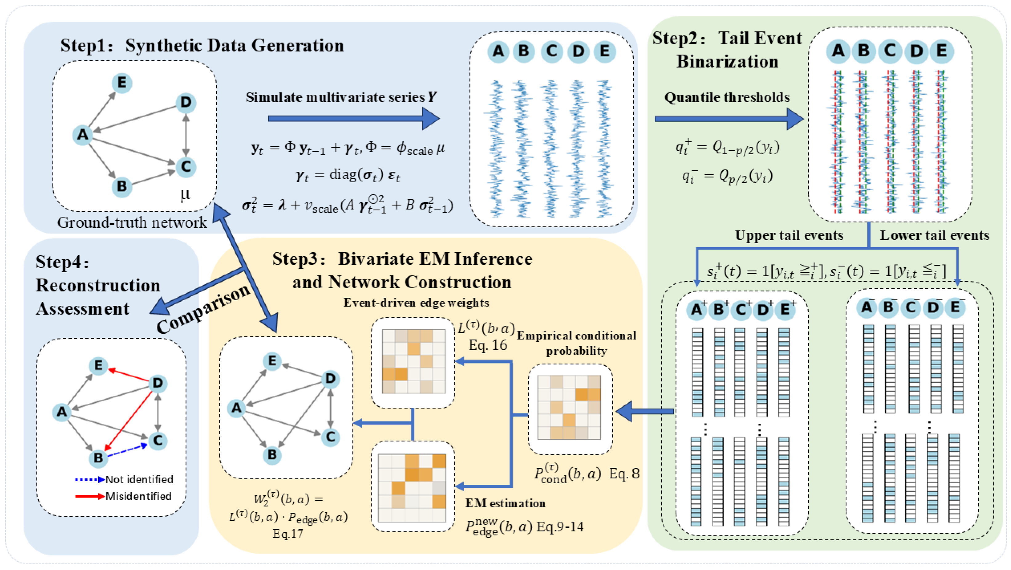Figure 2 outlines the four steps of the framework: generating synthetic time series, encoding extreme fluctuations as upper and lower tail outlier indicators through quantile thresholds, applying bivariate EM-based inference to reconstruct the underlying directed network, and assessing reconstruction quality by comparing the inferred network with the ground truth and with representative econometric baselines. In simulation studies, we evaluate reconstruction quality (precision, recall, and F1), and benchmark ODNI against three representative baselines: CoVaR, Clayton copula, and DCC-GARCH. Finally, we further apply ODNI to real-market data to reconstruct Tail Outlier-Triggering Networks in two settings: major foreign exchange rates and major global stock indices.

ODNI infers directional triggering links from upper and lower tail outliers and distinguishes among upper-to-upper, lower-to-lower, upper-to-lower, and lower-to-upper triggering channels. These channels provide a detailed view of tail state transmission, reversal, and switching dynamics under extreme market conditions. The proposed framework offers a systematic way to uncover latent tail risk transmission pathways from repeated lagged tail event relationships, providing implications for systemic risk monitoring and early warning.

2. Materials and Methods

To provide a controlled proxy for real-world markets, we first specify a directed weighted interaction template and simulate multivariate financial time series with volatility clustering and cross-variable spillovers. Figure 2 summarizes the ODNI workflow in four steps.

2.1. Synthetic Data Generation

Modeling financial time series is a challenging task, as such data are known to exhibit noisy dynamics, high volatility, excess kurtosis, volatility clustering, heavy tails, and non-stationarity [24,45,46,47,48]. The Generalized Autoregressive Conditional Heteroskedasticity (GARCH) model is widely used to characterize time-varying volatility and volatility clustering [49]. To generate synthetic multivariate time series with a known ground-truth network structure, we first specify a directed weighted interaction template $\mu \in {\mathbb{R}}^{n\times n}$. The synthetic series $y_t\in {\mathbb{R}}^n$ is generated by a cross-GARCH(1,1):

$${\mathbf{y}}_t=\mathsf{\Phi }\hspace{0.17em}{\mathbf{y}}_{t-1}+{\mathit{\gamma }}_t,\mathsf{\Phi }={\varphi }_{\mathrm{s}\mathrm{c}\mathrm{a}\mathrm{l}\mathrm{e}}\hspace{0.17em}\mu ,$$

(1)

Here, ${\varphi }_{\mathrm{scale}}>0$ controls the overall strength of the network. The off-diagonal non-zero entries ${\mu }_{ij}(i\ne j)$ define directed influences $j \to i$ and serve as the “answer” network in simulation studies. For stability, we enforce $\rho \left(\mathsf{\Phi }\right)<1$ (spectral radius), implemented by scaling $\mathsf{\Phi }$ when necessary.

To reproduce volatility clustering and cross-variable spillovers, we model the conditional variance vector ${\mathit{\sigma }}_t^2=({\sigma }_{1,t}^2,\dots ,{\sigma }_{n,t}^2{)}^{\mathrm{\top }}$ using a cross-GARCH(1,1) form:

$${\mathit{\sigma }}_t^2=\mathit{\lambda }+v_{\mathrm{s}\mathrm{c}\mathrm{a}\mathrm{l}\mathrm{e}}(A\hspace{0.17em}{\mathit{\gamma }}_{t-1}^{\odot 2}+B\hspace{0.17em}{\mathit{\sigma }}_{t-1}^2)$$

(2)

where $\lambda \in {\mathbb{R}}^n$ is a positive constant vector; $A=\left[a_{ij}\right]\in {\mathbb{R}}^{n\times n}$ and $B=\left[b_{ij}\right]\in {\mathbb{R}}^{n\times n}$ are coefficient matrices; and ${\mathit{\gamma }}_{t-1}^{\odot 2}\equiv {\mathit{\gamma }}_{t-1}\odot {\mathit{\gamma }}_{t-1}$ and $v_{\mathrm{scale}}>0$ control the overall strength of volatility spillovers. In component form

$${\sigma }_{i,t}^2={\lambda }_i+v_{\mathrm{scale}}\left({\displaystyle {\sum }_{j=1}^n}{a}_{ij}{\gamma }_{j,t-1}^2+{\displaystyle {\sum }_{j=1}^n}{b}_{ij}{\sigma }_{j,t-1}^2\right)$$

(3)

Volatility stability is ensured by constraining the effective persistence of each row, i.e., $v_{\mathrm{s}\mathrm{c}\mathrm{a}\mathrm{l}\mathrm{e}}\cdot \underset{i}{\mathrm{m}\mathrm{a}\mathrm{x}}{\displaystyle {\sum }_{j=1}^n}(a_{ij}+b_{ij})<1$, during implementation, while scaling $A$ and $B$ if necessary so that this condition holds. The innovation term is generated as

$${\mathit{\gamma }}_t=\mathrm{d}\mathrm{i}\mathrm{a}\mathrm{g}\left({\mathit{\sigma }}_t\right)\hspace{0.17em}{\mathit{\epsilon }}_t,{\gamma }_{i,t}={\sigma }_{i,t}{\epsilon }_{i,t},$$

(4)

where ${\sigma }_{i,t}=\sqrt{{\sigma }_{i,t}^2}$. The noise ${\epsilon }_{i,t}$ is i.i.d. with zero mean and unit variance; we use ${\epsilon }_{i,t}\sim \mathcal{N}\left(\mathrm{0,1}\right)$ as a baseline and an optional standardized Student-$t$ distribution (unit variance) to induce heavier tails. For numerical stability, the simulation also applies mild clipping to ${\mathit{\sigma }}_t^2$ and ${\mathit{\gamma }}_t$. We initialize ${\mathbf{y}}_0$ randomly (or user-specified) and set ${\mathit{\sigma }}_0^2$ near its unconditional level; a burn-in period is discarded to reduce dependence on initialization.

Equations (1)–(4) jointly generate multivariate sequences that exhibit both network-driven mean dependence and volatility clustering, while keeping a known ground-truth mean network template (equivalently $\mathsf{\Phi }$ and $\mu$) available for evaluating ODNI’s network reconstruction performance.

2.2. Outlier-Based Tail Encoding

ODNI operates on an outlier-based binary representation that isolates rare extreme fluctuations in each series. We encode upper and lower tail outliers using empirical quantiles, which are robust to skewness and heavy tails while providing a controllable activation rate across nodes.

We let ${\mathbf{y}}_t=(y_{1,t},\dots ,y_{n,t}{)}^{\mathrm{\top }}$ denote the simulated (or observed) multivariate series. For each node $i$, we fix a total tail probability $p\in \left(\mathrm{0,1}\right)$ and compute the lower and upper empirical quantiles as

$$q_i^{-}=Q_{{\displaystyle \frac{p}{2}}}(\{y_{i,t}{\}}_{t=1}^T),q_i^{+}=Q_{1-{\displaystyle \frac{p}{2}}}(\{y_{i,t}{\}}_{t=1}^T)$$

(5)

where $Q_{\alpha }(\cdot )$ denotes the $\alpha$-quantile. We then define upper and lower tail outlier indicators that distinguish upper tail and lower tail extremes:

$$s_i^{+}\left(t\right)=1[y_{i,t}\ge q_i^{+}],s_i^{-}\left(t\right)=1[y_{i,t}\le q_i^{-}]$$

(6)

This construction yields two tail channels per node, corresponding to upper tail and lower tail outliers and prevents cancelation of opposite-sign extremes when subsequent inference aggregates across time. We concatenate these channels to form an outlier activation matrix:

$$S_2=\left[\begin{array}{c}s(t,k)\end{array}\right]\in \{\mathrm{0,1}{\}}^{T\times 2n},s(t,i)=s_i^{+}(t),s(t,n+i)=s_i^{-}(t),i=1,\dots ,n.$$

(7)

Thus, the first $n$ columns of $S_2$ correspond to upper tail outliers, and the last $n$ columns correspond to lower tail outliers. The parameter $p$ directly controls the expected sparsity of activations; under continuity, $\mathbb{E}\left[s_i^{+}\right(t\left)\right]\approx p/2$ and $\mathbb{E}\left[s_i^{-}\right(t\left)\right]\approx p/2$, so each node contributes approximately a fraction $p$ of tail outliers in total. In practice, ties can occur in finite samples (especially under discretization or strong volatility clustering); we break ties deterministically by the empirical quantile rule so that the realized activation rate remains close to $p$.

The outlier activation matrix $S_2$ is the direct input to ODNI’s pairwise inference step. For a chosen lag $\tau$, ODNI estimates whether a tail outlier in a source channel (upper or lower) at time $t$ increases the probability of a tail outlier in a target channel at time $t+\tau$. When reporting a final $n\times n$ directed network over original nodes, the inferred tail channel interactions can be aggregated back to node-level connections, while retaining the benefits of upper/lower tail encoding during estimation.

This continuous-to-binary transformation defines the tail event representation used by ODNI. After this step, the model works with upper and lower tail activation sequences. The transformation preserves the occurrence, sign, and timing of extreme states, which provide the input information for identifying lagged triggering patterns in the subsequent inference step. Ordinary non-tail fluctuations and the relative magnitude of observations beyond the tail threshold are not encoded in this binary representation. The resulting activation matrix is then used as the direct input for the bivariate EM inference described in the next subsection.

2.3. Bivariate EM Inference

Given the outlier activation matrix $S_2=\left[s\right(t,k\left)\right]\in \{\mathrm{0,1}{\}}^{T\times 2n}$, ODNI infers a directed probabilistic triggering structure among upper and lower tail outlier channels. We adopt a bivariate statistical inference scheme estimated via an Expectation–Maximization (EM) model [42] and tailor it to upper and lower tail outliers. Each column of $S_2$ corresponds to a triggerable tail label, representing either an upper tail outlier or a lower tail outlier of a node. For a chosen lag $\tau \ge 1$, the objective is to quantify how a trigger $a$ at time $t$ contributes to a response $b$ at time $t+\tau$. We let $K=2n$ denote the number of tail labels, indexed by $a,b\in \{1,\dots ,K\}$.

(1)

Observable lagged conditional activation probability

For each ordered pair (a, b) with $a\ne b$, we first compute an empirical conditional probability that the target channel activates $\tau$ steps later, given that the source is active while the target is currently inactive:

$$P_{\mathrm{c}\mathrm{o}\mathrm{n}\mathrm{d}}^{\left(\tau \right)}\left(b,a\right)=\mathbb{P}\left[s\left(t+\tau ,b\right)=1∣s\left(t,a\right)=1,s\left(t,b\right)=0\right]$$

(8)

In practice, $P_{\mathrm{c}\mathrm{o}\mathrm{n}\mathrm{d}}^{\left(\tau \right)}(b,a)$ is estimated by relative frequencies over time indices $t\in \{1,\dots ,T-\tau \}$ that satisfy the conditioning set. This term captures a raw lag-$\tau$ association between tail channels, but by itself it does not distinguish direct effects from indirect pathways or common drivers.

(2)

Latent attribution model with spontaneous activations

ODNI assumes that when the target channel $b$ becomes active at $t+\tau$ while currently inactive at $t$, the activation can be attributed either to (i) one of the other channels $a\ne b$ that are active at time $t$, or (ii) a spontaneous mechanism specific to the target. We represent the probability that $a$ is the direct trigger of $b$ by a latent parameter as

$$P_{\mathrm{e}\mathrm{d}\mathrm{g}\mathrm{e}}\left(b,a\right)\in \left[0,1\right],a\ne b$$

(9)

and include a target-specific spontaneous activation rate ${\epsilon }_b\in [0, 1]$.

For each target channel $b$, inference is performed only on time indices where the target is currently inactive:

$${\mathcal{T}}_b=\left\{t\in \left\{1,\dots ,T-\tau \right\}:s\left(t,b\right)=0\right\}$$

(10)

This conditioning makes the attribution interpretation well defined because it focuses on which source contributes to the next activation of $b$. It also avoids trivial cases in which the target is already active.

We define the lag-$\tau$ activation intensity of the target channel $b$ at time $t+\tau$ as,

$${\mathsf{\Lambda }}_b\left(t\right)={\epsilon }_b+\sum _{a\ne b}{P}_{\mathrm{e}\mathrm{d}\mathrm{g}\mathrm{e}}\left(b,a\right)\hspace{0.17em}{P}_{\mathrm{c}\mathrm{o}\mathrm{n}\mathrm{d}}^{\left(\tau \right)}\left(b,a\right)\hspace{0.17em}s\left(t,a\right),t\in {\mathcal{T}}_b$$

(11)

Here, $P_{\mathrm{c}\mathrm{o}\mathrm{n}\mathrm{d}}^{\left(\tau \right)}(b,a)\hspace{0.17em}s(t,a)$ acts as an exposure-weighted contribution from channel $a$, while ${\epsilon }_b$ captures spontaneous activations of $b$ that are not attributable to any observed source channel at time $t$.

(3)

EM estimation

We let $y_b\left(t\right)=s(t+\tau ,b)$ denote whether the target activates at $t+\tau$. ODNI estimates $\left\{P_{\mathrm{e}\mathrm{d}\mathrm{g}\mathrm{e}}(b,a){\}}_{a\ne b}\right.$ and ${\epsilon }_b$ via an EM procedure are applied separately for each target $b$.

E-step (responsibilities). For each $t\in {\mathcal{T}}_b$, we compute the posterior responsibility that source channel $a$ accounts for an activation of $b$:

$${\rho }_{b\leftarrow a}\left(t\right)={\displaystyle \frac{P_{\mathrm{e}\mathrm{d}\mathrm{g}\mathrm{e}}\left(b,a\right)\hspace{0.17em}{P}_{\mathrm{c}\mathrm{o}\mathrm{n}\mathrm{d}}^{\left(\tau \right)}\left(b,a\right)\hspace{0.17em}s\left(t,a\right)}{{\mathsf{\Lambda }}_b\left(t\right)}},{\rho }_{b\leftarrow \epsilon }\left(t\right)={\displaystyle \frac{{\epsilon }_b}{{\mathsf{\Lambda }}_b\left(t\right)}}$$

(12)

Intuitively, ${\rho }_{b\leftarrow a}\left(t\right)$ is large when channel $a$ is active at $t$, the observed lagged conditional probability from $a$ to $b$ is high, and the current model assigns a large attribution weight to $a$.

M-step (parameter updates). Parameters are updated by maximizing the expected complete data likelihood. For each $a\ne b$,

$$P_{\mathrm{e}\mathrm{d}\mathrm{g}\mathrm{e}}^{\mathrm{n}\mathrm{e}\mathrm{w}}\left(b,a\right)={\displaystyle \frac{{\sum }_{t\in {\mathcal{T}}_b}{y}_b\left(t\right)\hspace{0.17em}{\rho }_{b\leftarrow a}\left(t\right)}{{\sum }_{t\in {\mathcal{T}}_b}{P}_{\mathrm{c}\mathrm{o}\mathrm{n}\mathrm{d}}^{\left(\tau \right)}\left(b,a\right)\hspace{0.17em}s\left(t,a\right)}}$$

(13)

and the spontaneous rate is updated by

$${\epsilon }_b^{\mathrm{n}\mathrm{e}\mathrm{w}}={\displaystyle \frac{{\sum }_{t\in {\mathcal{T}}_b}{y}_b\left(t\right)\hspace{0.17em}{\rho }_{b\leftarrow \epsilon }\left(t\right)}{\mid {\mathcal{T}}_b\mid }}$$

(14)

The numerator $\sum y_b\left(t\right){\rho }_{b\leftarrow a}\left(t\right)$ is the expected number of activations of $b$ attributed to source $a$, whereas the denominator $\sum P_{\mathrm{c}\mathrm{o}\mathrm{n}\mathrm{d}}^{\left(\tau \right)}(b,a)s(t,a)$ represents the expected exposure of $b$ to source $a$ under the lag-$\tau$ conditioning. If this denominator is zero (i.e., the pair $\left(a,b\right)$ has no effective exposures in the data), the edge parameter is not identifiable and is set to zero. We iterate E/M steps until convergence (or a maximum number of iterations), and we set $P_{\mathrm{e}\mathrm{d}\mathrm{g}\mathrm{e}}(b,b)=0$ by convention.

(4)

Outputs of the bivariate EM inference

ODNI produces three $K\times K$ matrices, all with zero diagonal. $P_{\mathrm{c}\mathrm{o}\mathrm{n}\mathrm{d}}^{\left(\tau \right)}$ contains the observable lagged conditional activation probabilities defined in Equation (8). $P_{\mathrm{e}\mathrm{d}\mathrm{g}\mathrm{e}}$ contains the EM-estimated direct attribution probabilities defined in Equations (9)–(14). $P_{\mathrm{e}\mathrm{f}\mathrm{f}}^{\left(\tau \right)}$ contains the effective activation probabilities defined in Equation (15).

$$P_{\mathrm{e}\mathrm{f}\mathrm{f}}^{\left(\tau \right)}\left(b,a\right)=P_{\mathrm{c}\mathrm{o}\mathrm{n}\mathrm{d}}^{\left(\tau \right)}\left(b,a\right)\cdot P_{\mathrm{e}\mathrm{d}\mathrm{g}\mathrm{e}}\left(b,a\right)$$

(15)

In addition, ODNI outputs the spontaneous activation vector $\mathit{\epsilon }=({\epsilon }_1,\dots ,{\epsilon }_K{)}^{\mathrm{\top }}$. These quantities provide the basis for constructing a tail channel-triggering network at temporal scale $\tau$. Section 2.4 further converts these outputs into the final ODNI edge score and describes how tail channel interactions are aggregated into an $n\times n$ node-level directed network.

2.4. Outlier-Driven Network Construction

The bivariate EM step provides the observable lagged conditional probabilities $P_{\mathrm{c}\mathrm{o}\mathrm{n}\mathrm{d}}^{\left(\tau \right)}$, the EM attribution weights $P_{\mathrm{e}\mathrm{d}\mathrm{g}\mathrm{e}}$, and the spontaneous activation vector $\mathit{\epsilon }$. We adopt the convention that rows index response channels $b$ and columns index trigger channels $a$.

Based on these quantities, ODNI constructs a weighted directed network on upper and lower tail channels. In this paper, this network is referred to as a Tail Outlier-Triggering Network, because its edges are estimated from repeated lagged activation patterns among tail outliers. When an asset-level network is required for visualization or performance evaluation, the tail channel network is further mapped back to a directed node-level network over the original assets.

(1) Outlier-driven network.

We first define edge weights between upper and lower tail outliers. To remove the spontaneous background of each response channel $b$, we compute a non-negative excess conditional probability:

$$L^{\left(\tau \right)}(b,a)=max\left(0,P_{\mathrm{c}\mathrm{o}\mathrm{n}\mathrm{d}}^{\left(\tau \right)}(b,a)-{\epsilon }_b\right)$$

(16)

We then combine this excess component with the EM attribution weight to obtain the tail channel’s edge weight matrix $W_2^{\left(\tau \right)}\in {\mathbb{R}}^{K\times K}$:

$$W_2^{\left(\tau \right)}\left(b,a\right)=L^{\left(\tau \right)}\left(b,a\right)\cdot P_{\mathrm{e}\mathrm{d}\mathrm{g}\mathrm{e}}\left(b,a\right),a\ne b$$

(17)

and we set $W_2^{\left(\tau \right)}(b,b)=0$ by convention.

When an $n\times n$ directed network over the original nodes is required (e.g., for visualization or comparison with baselines), we convert tail channel weights to node-to-node weights. Each node $i$ has two tail labels: an upper tail outlier and a lower tail outlier. We let $i^{+}$ and $i^{-}$ denote their indices. For a directed link $i \to j$ at lag $\tau$, we compute same-tail triggering (upper-to-upper and lower-to-lower),

$$W_{\mathrm{s}\mathrm{a}\mathrm{m}\mathrm{e}}^{\left(\tau \right)}\left(j,i\right)=W_2^{\left(\tau \right)}\left(j^{+},i^{+}\right)+W_2^{\left(\tau \right)}\left(j^{-},i^{-}\right)$$

(18)

as well as cross-tail triggering (upper-to-lower and lower-to-upper),

$$W_{\mathrm{f}\mathrm{l}\mathrm{i}\mathrm{p}}^{\left(\tau \right)}\left(j,i\right)=W_2^{\left(\tau \right)}\left(j^{+},i^{-}\right)+W_2^{\left(\tau \right)}\left(j^{-},i^{+}\right)$$

(19)

These channel-specific links are not mutually exclusive. For the same ordered asset pair $i \to j$, an upper tail outlier in asset $i$ may be followed by an upper tail outlier in asset $j$ in some historical episodes, and by a lower tail outlier in asset $j$ in other episodes. Thus, $i^{+} \to j^{+}$ and $i^{+} \to j^{-}$ summarize different target tail responses that are conditional on the same source tail state. Their coexistence indicates state-dependent tail responses across different market episodes.

ODNI retains the dominant triggering mode and defines the node-to-node edge weight matrix $W^{\left(\tau \right)}\in {\mathbb{R}}^{n\times n}$ as

$$W^{\left(\tau \right)}\left(j,i\right)=\max \left(W_{\mathrm{s}\mathrm{a}\mathrm{m}\mathrm{e}}^{\left(\tau \right)}\left(j,i\right),W_{\mathrm{f}\mathrm{l}\mathrm{i}\mathrm{p}}^{\left(\tau \right)}\left(j,i\right)\right),i\ne j$$

(20)

where $W^{\left(\tau \right)}(i,i)=0$. This aggregation is used when a single asset-level directed score is needed. In empirical interpretation, however, the four channel-specific networks can also be retained separately, because they reveal different tail response mechanisms, including same-tail continuation, downside co-movement, cross-tail reversal, hedging, and market switching.

(2) Performance evaluation.

In the simulation experiments, the ground-truth network is defined at the asset level by the non-zero off-diagonal entries of the directed interaction template. ODNI first estimates triggering relationships at the tail channel level, so the four channel-level triggering modes are aggregated into a node-level edge score before evaluation. The resulting $W\left(j,i\right)$ represents the strongest tail outlier-triggering evidence from asset $i$ to asset $j$. This node-level score is then thresholded to obtain a binary directed graph.

To extract a binary directed graph from $W^{\left(\tau \right)}$, we apply a threshold $\theta$:

$${\widehat{A}}_{j,i}^{\left(\tau \right)}=1\left[W^{\left(\tau \right)}\left(j,i\right)\ge \theta \right],i\ne j$$

(21)

In simulation studies where the ground-truth adjacency matrix $A$ is known (diagonal excluded), we scan a set of candidate thresholds and choose $\theta$ that maximizes the F1 score. For stability, we use a quantile-based grid over off-diagonal weights. Given $\widehat{A}$ and $A$, we compute TP, FP, FN, and TN over off-diagonal entries and report:

$$\mathrm{P}\mathrm{r}\mathrm{e}\mathrm{c}\mathrm{i}\mathrm{s}\mathrm{i}\mathrm{o}\mathrm{n}={\displaystyle \frac{\mathrm{T}\mathrm{P}}{\mathrm{T}\mathrm{P}+\mathrm{F}\mathrm{P}}},$$

(22)

$$\mathrm{R}\mathrm{e}\mathrm{c}\mathrm{a}\mathrm{l}\mathrm{l}={\displaystyle \frac{\mathrm{T}\mathrm{P}}{\mathrm{T}\mathrm{P}+\mathrm{F}\mathrm{N}}},$$

(23)

$$\mathrm{F}\mathrm{P}\mathrm{R}={\displaystyle \frac{\mathrm{F}\mathrm{P}}{\mathrm{F}\mathrm{P}+\mathrm{T}\mathrm{N}}},$$

(24)

$$\mathrm{F}1={\displaystyle \frac{2\mathrm{P}\mathrm{r}\mathrm{e}\mathrm{c}\mathrm{i}\mathrm{s}\mathrm{i}\mathrm{o}\mathrm{n}\cdot \mathrm{R}\mathrm{e}\mathrm{c}\mathrm{a}\mathrm{l}\mathrm{l}}{\mathrm{P}\mathrm{r}\mathrm{e}\mathrm{c}\mathrm{i}\mathrm{s}\mathrm{i}\mathrm{o}\mathrm{n}+\mathrm{R}\mathrm{e}\mathrm{c}\mathrm{a}\mathrm{l}\mathrm{l}}}$$

(25)

When scanning thresholds, precision–recall tradeoffs vary with $\theta$; therefore, we use the best F1 threshold as the primary operating point in simulation comparisons, and report the corresponding precision/recall/F1 together with the selected $\theta$.

2.5. Comparative Methods

To contextualize ODNI, we compare it with three representative dependence-based approaches that are commonly used in financial risk analysis. CoVaR- and copula-based dependence are classic tools for characterizing co-movement under heavy tails and extreme observations, with copulas providing an explicit tail-dependent measure. DCC-GARCH is included as a canonical extension within the GARCH family, capturing volatility clustering together with time-varying conditional correlations. All methods are applied to the same input series and output a weighted network $W\in {\mathbb{R}}^{n\times n}$.

(1)

CoVaR (tail risk spillover baseline)

We let $y_{i,t}$ be the return of node $i$ and $L_{i,t}=-y_{i,t}$ be the loss. The $q$-level VaR of node $i$ is ${\mathrm{V}\mathrm{a}\mathrm{R}}_i^{\left(q\right)}=Q_q\left(\right\{L_{i,t}{\}}_{t=1}^T)$. We define ${\mathrm{C}\mathrm{o}\mathrm{V}\mathrm{a}\mathrm{R}}_{j\mid i}^{\left(q\right)}$ as the $q$-quantile of $L_{j,t}$ conditional on node $i$ being in distress, i.e., $L_{i,t}\ge {\mathrm{V}\mathrm{a}\mathrm{R}}_i^{\left(q\right)}$:

$${\mathrm{C}\mathrm{o}\mathrm{V}\mathrm{a}\mathrm{R}}_{j\mid i}^{\left(q\right)}=Q_q\left(\left\{L_{j,t}:L_{i,t}\ge {\mathrm{V}\mathrm{a}\mathrm{R}}_i^{\left(q\right)}\right\}\right)$$

(26)

A directed CoVaR network is constructed with weights $W_{j,i}=\mid {\mathrm{C}\mathrm{o}\mathrm{V}\mathrm{a}\mathrm{R}}_{j\mid i}^{\left(q\right)}\mid$ and $W_{i,i}=0$. Larger $W_{j,i}$ indicates stronger downside loss of $j$ during distress of $i$.

(2)

Clayton copula tail-dependent network.

To explicitly focus on dependence in extremes, we fit a bivariate Clayton copula pairwise and use its lower tail dependence as the network weight. Using pseudo-observations $u_{i,t}=\mathrm{r}\mathrm{a}\mathrm{n}\mathrm{k}\left(y_{i,t}\right)/(T+1)$, the Clayton copula is

$$C\left(u,v∣\theta \right)={\left(\max \left\{u^{-\theta }+v^{-\theta }-1,\hspace{0.17em}0\right\}\right)}^{-{\displaystyle \frac{1}{\theta }}},\theta >0.$$

(27)

Its implied lower tail dependence coefficient is ${\lambda }_L=2^{-1/\theta }.$

We define $W_{ij}={\lambda }_L$ for $i\ne j$ (and $W_{ii}=0$), yielding an undirected tail risk dependence network that emphasizes joint downside extremes. We include this baseline because copulas provide a principled way to separate tail dependence from central dependence, making them a standard choice for modeling systemic risk and extreme co-movements.

(3)

Dynamic conditional correlation network (DCC-GARCH)

Financial returns exhibit volatility clustering, i.e., time-varying conditional variance. GARCH models capture this feature, and DCC-GARCH extends the GARCH family to multivariate settings by additionally modeling time-varying conditional correlations. Fitting a DCC-GARCH model yields a sequence of conditional correlation matrices $R_t$. We construct a static network by temporal aggregation of the conditional correlations:

$$W_{ij}={\displaystyle \frac{1}{T}}{\displaystyle \sum _{t=1}^T}\mid (R_t{)}_{ij}\mid ,i\ne j,$$

(28)

with $W_{ii}=0$. We include DCC-GARCH as a representative GARCH family baseline; it is widely used in volatility spillover and systemic risk studies, and it provides a dynamic dependence benchmark that complements the outlier-driven perspective of ODNI.

3. Network Reconstruction from Synthetic Data

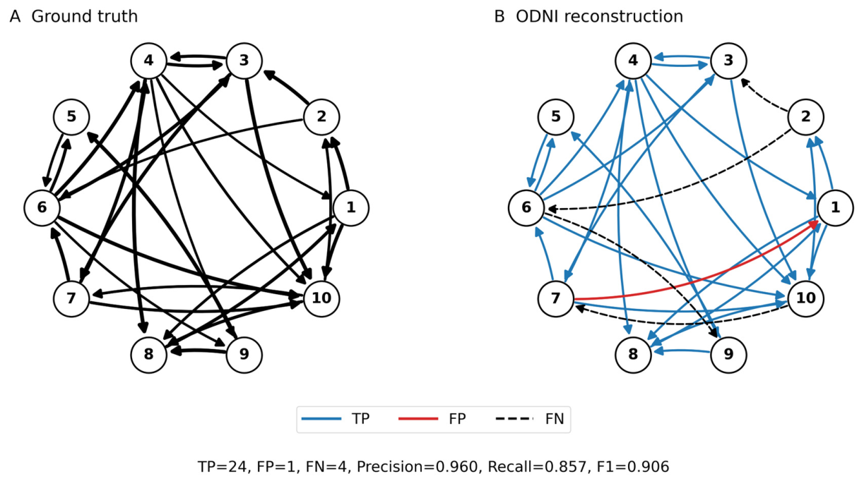
Figure 3 presents a representative network reconstruction result based on the synthetic data. Since ODNI first estimates triggering relationships at the tail channel level, the four tail-triggering channels need to be aggregated into a node-level directed network before comparison with the ground-truth network. Figure 3B shows the aggregated ODNI reconstruction.

In the representative run shown in Figure 3 ($N=10$, lag = 1), the ground-truth network contains 28 directed links. ODNI correctly recovers 24 links, introduces one false positive, and misses four true links, yielding precision = 0.960, recall = 0.857, and F1 = 0.906 at the displayed threshold. These results indicate that ODNI captures most of the underlying directed structure while maintaining a low false positive rate. The remaining missed links suggest that some weaker or less frequently activated interactions are more difficult to recover from finite-sample tail events. Therefore, this example should be interpreted as a representative topology recovery case rather than a perfect reconstruction. For application purposes, ODNI is better viewed as a conservative tool for identifying major tail-triggering pathways, especially when repeated lagged tail activations are sufficiently observable.

3.1. Model Comparison

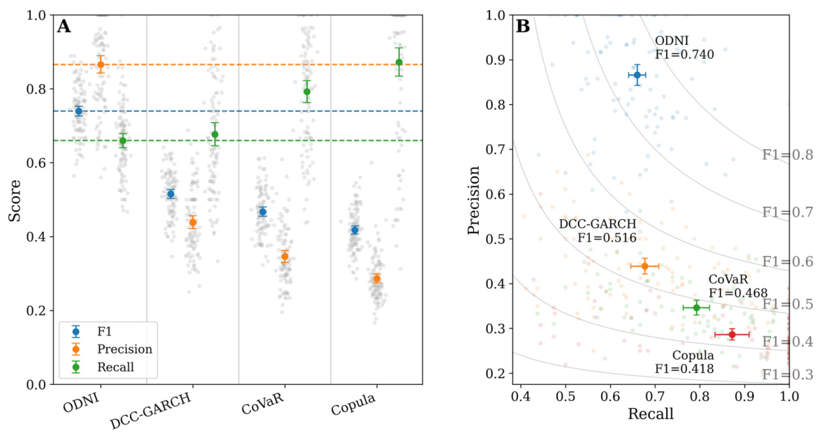
We next benchmark ODNI against three widely used baselines: DCC-GARCH, CoVaR, and a copula tail-dependent network. All methods are evaluated on the same synthetic datasets and against the same known ground-truth networks. To ensure a fair comparison despite differences in score scales across methods, we adopt a consistent thresholding protocol. Within each run, we scan candidate thresholds; select the best F1 threshold that maximizes the F1 score; and then compute precision, recall, and F1 against the ground-truth adjacency matrix. We repeat this procedure over 100 independent runs and summarize the mean performance and variability across runs.

Overall, ODNI achieves the best network reconstruction performance among the compared methods. ODNI attains a mean F1 of 0.740, with mean precision 0.866 and mean recall 0.660, exhibiting a clear high-precision, moderate-recall profile. In contrast, DCC-GARCH yields a mean F1 of 0.516, with precision 0.439 and recall 0.677; CoVaR yields a mean F1 of 0.468, with precision 0.346 and recall 0.793; and the copula tail-dependence network yields a mean F1 of 0.418, with precision 0.287 and recall 0.872. These results indicate that CoVaR and copula-based approaches often achieve higher recall by producing much denser inferred networks, but at the cost of substantially lower precision due to many false positives, which depresses the overall F1 score. Figure 4B further shows that ODNI maintains consistently higher precision across runs and therefore achieves the best F1, even though its recall is not the highest.

The run-wise ODNI estimates concentrate in a high-precision region while maintaining non-trivial recall, placing them on more favorable iso-F1 contours. DCC-GARCH typically occupies a mid-recall but low-precision region, whereas CoVaR and copula tail dependence cluster in a high-recall, low-precision region, consistent with systematic over-connection. From a network reconstruction perspective, ODNI does not aim to maximize recall at all costs. Instead, its main advantage lies in strongly suppressing false positives while retaining a meaningful true positive rate, thereby producing a more reliable set of directed links.

These differences are consistent with the modeling objectives and outputs of the baselines. Copula tail dependence and CoVaR are designed to characterize stress co-movement or conditional tail risk exposure rather than to recover a sparse directed transmission graph. When evaluated under a directed adjacency recovery objective, they therefore tend to over-connect and yield low precision. DCC-GARCH captures time-varying second-moment dependence and can reflect common volatility regimes, but its dependence structure is fundamentally symmetric and thus provides limited directional information, which restricts its performance under directed ground truth. In contrast, ODNI is explicitly built on directional outlier-triggering evidence and lagged tail-triggering relationships. Its EM inference with baseline correction produces a more separable edge score distribution, which in turn leads to cleaner threshold networks.

Taken together, the benchmark results support ODNI as a conservative yet reliable method for network reconstruction from financial time series. Relative to tail-dependent baselines that favor high recall but frequently over-connect, ODNI delivers substantially higher precision and a better precision–recall balance, resulting in superior F1 performance and more stable threshold behavior.

3.2. Robustness Tests

To examine the stability of ODNI under different data and network conditions, we adopt a one-factor-at-a-time design. In each experiment, only one key factor varies while all others are kept at their default values. The gray dots show results from 100 independent runs, the solid curve reports the mean, and the shaded band indicates uncertainty around the mean. We also report the run-wise best F1 threshold and its mean trajectory to track how the optimal decision point shifts across regimes.

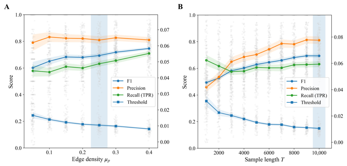
Figure 5A shows robustness to initial sparsity experiment, as the edge density ${\mu }_p$ increases from 0.05 to 0.40, while the mean precision stays consistently high within 0.79 to 0.83 and varies only slightly. This indicates that ODNI follows a conservative edge selection strategy and does not become unstable or generate an excessive number of false positives when the ground-truth network becomes denser. Meanwhile, as density increases, the mean recall rises overall, and the mean F1 improves steadily. This suggests that denser ground-truth networks provide more informative cross-node extreme event triggering pathways, yielding stronger and more frequent evidence for true directed links. The mean best F1 threshold decreases with ${\mu }_p$, indicating that when the base rate of true edges is higher, a lower cutoff can still maintain high precision while improving recall and F1.

Under the sample length experiment shown in Figure 5B, performance improves markedly as the sample length increases from 1000 to 10,000. Mean precision rises from a low level to about 0.81, whereas mean recall changes more moderately and stabilizes around 0.63, leading to a substantial increase in mean F1. This pattern shows that ODNI benefits primarily from stronger suppression of false positives when longer samples are available. Because outliers are rare, conditional probability estimates can be noisy in short series and may produce spuriously high-scoring edges, thereby lowering precision. As sample length increases, tail activation statistics become more stable, spurious edges are reduced, precision improves, and F1 increases accordingly. Consistently, the mean best F1 threshold decreases monotonically with sample length, reflecting improved score separability that allows a lower cutoff without introducing many false positives.

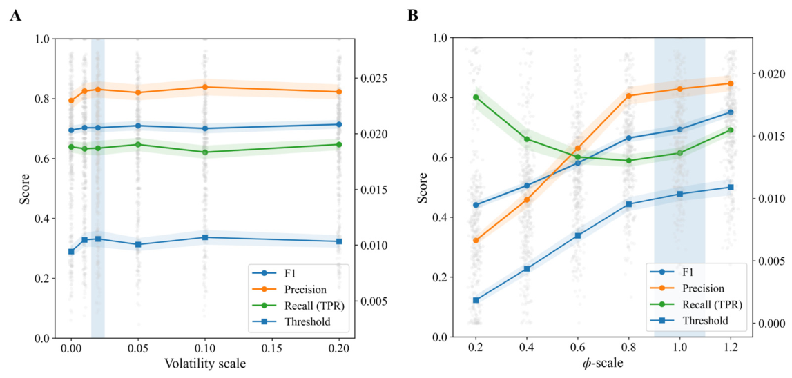
The effects of volatility scale and mean-network strength are further examined in Figure 6. Figure 6A reports the results of the volatility-scale experiment. ODNI is nearly insensitive to changes in volatility-noise strength over the range from 0 to 0.2. Mean precision remains stable between 0.79 and 0.84, mean recall stays between 0.62 and 0.65, mean F1 varies only slightly within a narrow range, and the mean best F1 threshold is also largely unchanged. This indicates that ODNI is not highly sensitive to changes in return amplitude or volatility level, because it operates on outlier-based tail indicators and depends on whether observations fall within tails rather than on their raw magnitudes. As a result, the method can accommodate substantial differences in volatility levels across assets or time periods.

As shown in Figure 6B, under the coupling strength experiment, as coupling strength increases from 0.2 to 1.2, overall recoverability improves substantially. Mean precision increases from a low level to around 0.85, and mean F1 rises accordingly. Though mean recall shows a decrease-then-recovery pattern, the key point is that at low coupling strength recall can appear high while precision is very low, indicating pervasive over-connection in the inferred network. As coupling strengthens, directional outlier-triggering patterns become clearer, spurious edges are strongly suppressed, precision improves, and F1 increases sharply. The mean best F1 threshold increases with coupling strength, reflecting an upward shift in the score distribution as true transmission signals strengthen, which moves the optimal cutoff to higher values.

Overall, ODNI can stably control false positives across a wide range of conditions while maintaining high precision with modest variability. When more identifiable information is available, either through longer samples or stronger true coupling, ODNI improves in a systematic and interpretable manner rather than relying on a narrow parameter sweet spot. ODNI can therefore be viewed as a conservative yet robust network reconstruction method that keeps false discoveries low while recovering a substantial fraction of true directed connections across regimes.

4. Outlier-Driven Network Inference in Financial Markets

We apply ODNI to real-market data to reconstruct directed tail-triggering networks in two settings: major foreign exchange rates and major stock indices. ODNI infers directional links from positive and negative tail outliers. For compact notation, positive-tail outliers are denoted as POS and negative-tail outliers are denoted as NEG. Accordingly, the empirical analysis distinguishes four tail-triggering channels: POS → POS, positive tail to positive tail-triggering; NEG → NEG, negative tail to negative tail-triggering; POS → NEG, positive tail to negative tail-triggering; and NEG → POS, negative tail to positive tail-triggering. In the following empirical discussion, POS → POS and NEG → NEG are interpreted as same-direction abnormal movement relationships, while POS → NEG and NEG → POS are interpreted as opposite-direction abnormal movement relationships.

4.1. Data and Validation

Foreign exchange market. The FX dataset consists of USD-based bilateral exchange rate series, denoted by the corresponding non-USD currency codes for simplicity: Australia (AUD), Canada (CAD), Switzerland (CHF), China (CNY), Euro area (EUR), United Kingdom (GBP), Hong Kong (HKD), Japan (JPY), Korea (KRW), Mexico (MXN), New Zealand (NZD), and Sweden (SEK). After aligning all series to common trading days and computing log returns, the resulting FX panel contains 8562 observations.

Stock indices market. The major stock indices: the Netherlands (AEX), Germany (DAX), U.S. Dow Jones (DJI), Hong Kong (HSI), Korea (KOSPI), U.S. Nasdaq (NDQ), Japan (NKX), China (SHC), Switzerland (SMI), U.S. S&P 500 (SPX), and Canada (TSX). After aligning all series to common trading days and computing log returns, the resulting index panel contains 7249 observations.

We complement the synthetic data validation with two empirical checks on the real-market panels: an out-of-sample conditional activation test to assess predictive content, and a randomized null model comparison to rule out random tail event alignment.

Table 1. Out-of-sample validation of ODNI-inferred tail-triggering links.

Market	Channel	Links	Baseline Probability	Conditional Probability	Lift	Share of Links with Lift > 1
FX	NEG → NEG	20	0.050	0.115	2.302	1.000
FX	NEG → POS	20	0.050	0.063	1.264	0.750
FX	POS → POS	20	0.050	0.102	2.034	0.800
FX	POS → NEG	20	0.050	0.063	1.258	0.650
INDEX	NEG → NEG	17	0.050	0.204	4.075	1.000
INDEX	NEG → POS	17	0.050	0.149	2.986	1.000
INDEX	POS → POS	17	0.050	0.113	2.254	0.824
INDEX	POS → NEG	17	0.050	0.069	1.370	0.529

reports the out-of-sample validation results. All channels in both markets have lift values greater than one, indicating that ODNI-inferred links increase the probability of future target tail activations. In the FX market, the strongest lift appears in the NEG → NEG channel, followed by POS → POS, suggesting that same-direction abnormal movement relationships are more prominent. In the stock index market, the validation results are stronger, especially for NEG → NEG, indicating that downside tail shocks have stronger predictive content for subsequent downside tail activations.

Table 2. Null model validation of ODNI-inferred links.

Market	Channel	Observed Lift	Randomized Mean Lift	Observed/Randomized	Empirical p-Value
FX	POS → POS	2.349	0.926	2.536	<0.01
FX	NEG → NEG	2.395	0.948	2.527	<0.01
FX	POS → NEG	2.624	0.966	2.717	<0.01
FX	NEG → POS	2.204	0.956	2.304	<0.01
INDEX	POS → POS	3.117	0.949	3.285	<0.01
INDEX	NEG → NEG	4.441	0.898	4.945	<0.01
INDEX	POS → NEG	1.878	0.909	2.067	<0.01
INDEX	NEG → POS	2.932	0.954	3.072	<0.01

reports the null model comparison. The observed lift values are consistently higher than the randomized benchmarks across all markets and channels. The observed-to-randomized ratios are all greater than two, and the empirical p-values are below 0.01. This suggests that the inferred empirical links are not simply caused by random tail co-occurrences, but reflect ordered lagged tail-triggering patterns in real financial markets.

These results provide empirical support for the real-market ODNI networks. The inferred links show positive out-of-sample predictive content and consistently exceed randomized tail event benchmarks. The following subsections further examine the channel-specific structures and economic interpretations of the FX and stock index networks.

4.2. Foreign Exchange Market

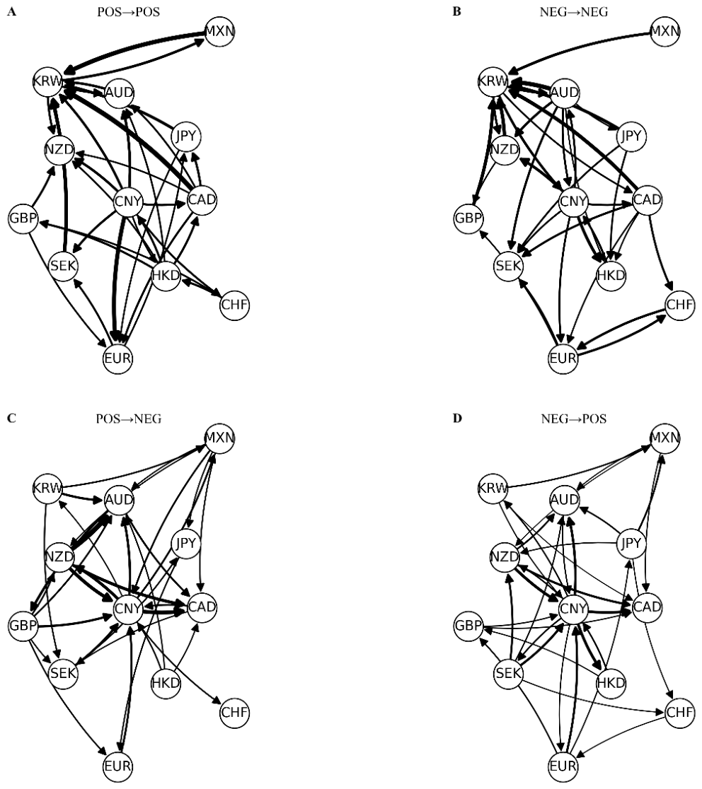
Figure 7 presents four channel-specific tail-triggering networks in the foreign exchange market. Overall, the FX network exhibits a clear regional structure, with an especially visible Asian cluster. Directional links among Asian exchange rate series are relatively dense, and the CNY, HKD, and KRW series occupy visible positions across different panels. The CNY-HKD linkage appears relatively stable, reflecting close exchange rate, trade, and financial connections between the Chinese mainland and Hong Kong. The KRW series receives a concentrated set of incoming links in the same-direction abnormal movement networks, indicating relatively high sensitivity to external extreme movements.

From Figure 7A,B, the KRW series shows a clear receiving role in same-direction abnormal movement relationships. When several other exchange rate series experience abnormal upward movements, the KRW series is more likely to show a subsequent abnormal upward movement. Similarly, when other series experience abnormal downward movements, the KRW series is also more likely to show a subsequent abnormal downward movement. Links from CAD, AUD, JPY, and MXN to KRW are visible in the same-direction networks, suggesting that the KRW series tends to act as a convergence point for external tail shocks in the FX network.

The CNY series shows a different pattern. In the abnormal upward-to-upward relationship, the CNY series is more outward-oriented; after an abnormal upward movement in the CNY series, several major exchange rate series also show subsequent abnormal upward movements. This suggests that the CNY series has a certain regional spillover role under upward extreme conditions. At the same time, CNY-related links also appear in opposite-direction abnormal movement relationships. After an abnormal upward movement in the CNY series, CAD and NZD show clearer abnormal downward responses, while AUD displays a more mixed pattern involving both same-direction continuation and opposite-direction adjustment. This shows that responses to CNY-related abnormal movements differ across target exchange rate series.

Figure 7C,D further show that opposite-direction abnormal movement relationships are more concentrated among a smaller group of exchange rate series. In the abnormal upward-to-downward relationship, the CNY series is more tilted toward a receiving role, while the KRW and NZD series are more outward-oriented. This suggests that abnormal upward movements in some exchange rate series may be followed by abnormal downward responses in the CNY series, which may be related to short-term correction, capital switching, or risk repricing in the FX market. In the abnormal downward-to-upward relationship, the CNY series has both incoming and outgoing links and is closer to a bidirectional position, while the AUD series is more tilted toward a receiving role. These results indicate that the role of the CNY series changes across different abnormal movement relationships: it is more outward-oriented in upward same-direction relationships, more receiving in upward-to-downward relationships, and more balanced in downward-to-upward relationships.

The relationships between the CNY series and the HKD, NZD, and AUD series further reflect this heterogeneity. After an abnormal downward movement in the CNY series, the HKD series shows both same-direction downward responses and opposite-direction upward responses. The NZD series is more concentrated in the same-direction downward relationship. After an abnormal upward movement in the CNY series, the AUD series shows both same-direction upward responses and opposite-direction downward responses. These patterns suggest that the same source exchange rate series can be associated with different target responses under different abnormal movement states. The channel-specific tail-triggering networks therefore help distinguish same-direction continuation, opposite-direction adjustment, and mixed response patterns.

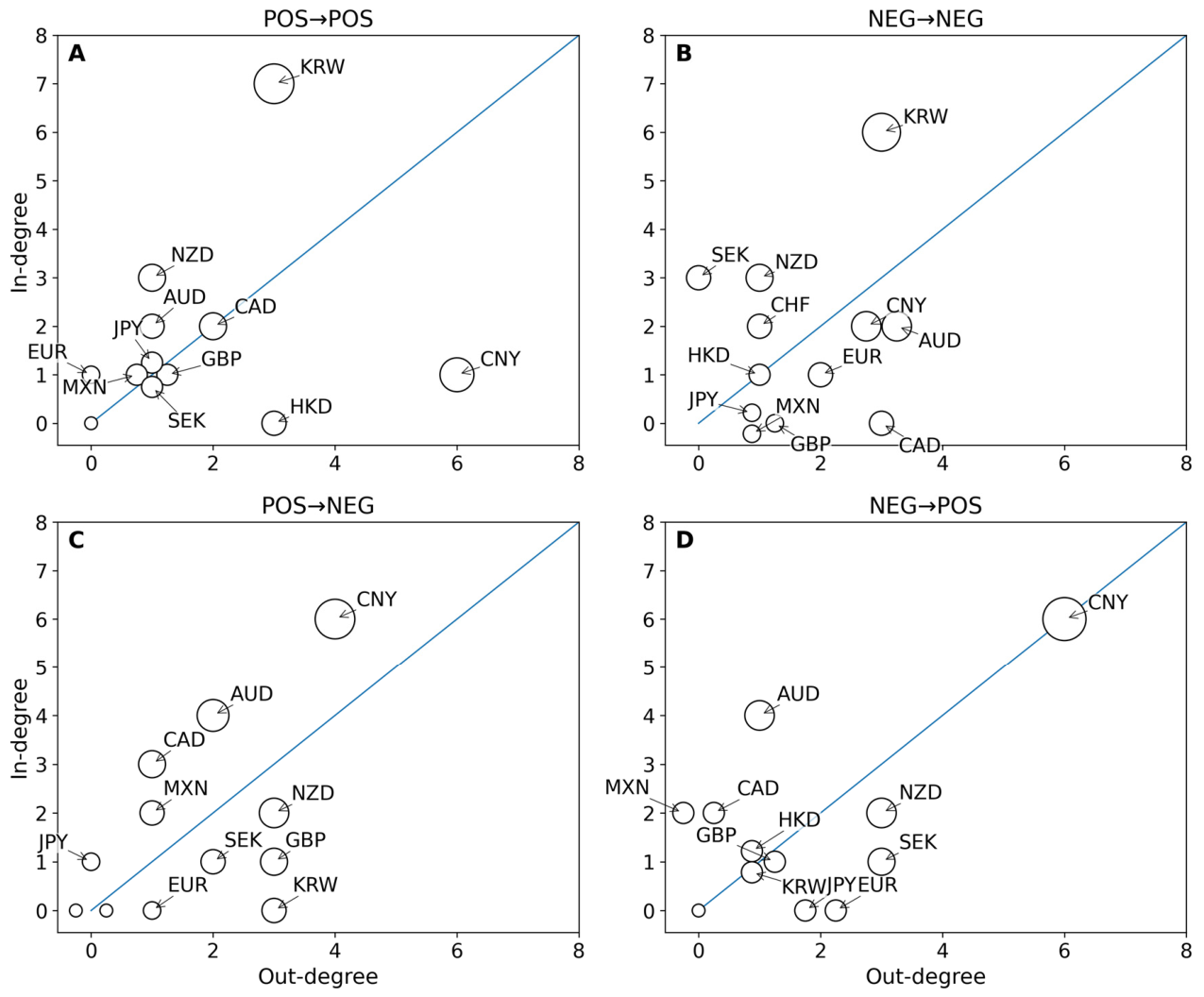
Figure 8 summarizes the above network patterns through in-degree and out-degree. In the same-direction abnormal movement relationships, the KRW series has relatively high in-degree, further confirming its receiving role. The CNY series shows a stronger outward role in the abnormal upward-to-upward relationship, consistent with the network structure in Figure 7. In the opposite-direction abnormal movement relationships, sender and receiver roles are more concentrated. The CNY series lies above the diagonal in the abnormal upward-to-downward relationship, indicating a stronger receiving role, while it lies closer to the diagonal in the abnormal downward-to-upward relationship, indicating a more balanced position. The AUD series is more receptive in the abnormal downward-to-upward relationship, while the NZD and KRW series are more outward-oriented in the abnormal upward-to-downward relationship.

These patterns are consistent with the heterogeneous roles of exchange rate series under extreme market conditions. Commodity-linked series, such as AUD, NZD, and CAD, are more exposed to global risk appetite and commodity-market conditions, so they appear more active in opposite-direction adjustment and hedging-related relationships. CNY-related exchange rate movements are influenced by regional trade, liquidity conditions, policy factors, and onshore–offshore market linkages, which helps explain their visible roles across both same-direction and opposite-direction relationships. The KRW series shows a relatively clear receiving role in same-direction abnormal movement relationships, reflecting its sensitivity to regional and global external shocks. Overall, the FX results show that channel-specific tail-triggering networks provide a more detailed description of tail risk transmission than a single aggregated exchange rate network, because they distinguish the direction and role of abnormal responses across different tail states.

4.3. Stock Index Market

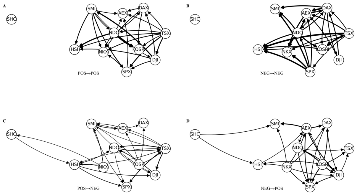
Figure 9 presents four channel-specific tail-triggering networks for major national and regional stock indices. Overall, the stock index network is more concentrated than the FX network. The United States and core European markets occupy central positions in several panels. Among the U.S. indices, the technology-oriented Nasdaq index shows a particularly visible outward role in downside-related relationships, while the broad U.S. market represented by the S&P 500 is more involved in cross-direction responses. Germany, Switzerland, and the Netherlands also form part of the main linkage structure. In contrast, the Chinese mainland market is weakly connected in most panels, while Hong Kong, China, shows a more visible role, especially in downside and cross-direction relationships.

From Figure 9 the same-direction abnormal movement relationships show different structures under upward and downward extreme conditions. In the abnormal downward-to-downward relationship, Hong Kong, China, receives links from multiple markets and behaves more like an absorbing endpoint for downside shocks. This indicates that when other major stock markets experience abnormal downward movements, Hong Kong, China, is more likely to show a subsequent abnormal downward response. By contrast, the U.S. technology-oriented Nasdaq index shows stronger outward connectivity in the same relationship, suggesting that downside abnormal movements in the U.S. technology market are more likely to be followed by downside responses in other markets.

The abnormal upward-to-upward relationship shows a different pattern. Canada appears closer to a sending role, while Hong Kong, China, and the United States show more receiving characteristics in this relationship. This suggests that upward extreme movements and downward extreme movements are not transmitted through the same market structure. The United States is not only a source of downside tail pressure; in some upward-related relationships, it also receives tail responses from other markets. This reflects the dual role of the U.S. market as both a global information source and a major destination for international capital adjustment.

The role of the United States is one of the most visible features of the stock index network. The Nasdaq-related structure appears in both upward and downward same-direction relationships, indicating that U.S. technology-market movements are closely connected with tail responses in other markets. Its links with Asian markets, including Hong Kong, China, and Korea, are especially noticeable. This suggests that the technology component of the U.S. market may serve as an important channel through which global risk sentiment and growth expectations are transmitted to Asian equity markets. The S&P 500 shows a more balanced role. It is connected to the main network structure, but its position varies across response types, especially in the cross-direction relationships.

Figure 9C,D show the opposite-direction abnormal movement relationships, which provide another view of market adjustment under extreme conditions. In the abnormal upward-to-downward relationship, Hong Kong, China, shows stronger outward connectivity. This suggests that abnormal upward movements related to Hong Kong, China, may be followed by abnormal downward responses in other markets during some episodes. In the abnormal downward-to-upward relationship, the United States, especially the broad market represented by the S&P 500, shows stronger incoming connectivity. This indicates that downside abnormal movements in other markets may be followed by upward abnormal responses in the U.S. market. These cross-direction patterns are more closely related to market adjustment, rebound, hedging, and cross-market reallocation under extreme conditions.

The China-related markets show a clear internal contrast. Hong Kong, China, is much more visible than the Chinese mainland market in the inferred networks. In the abnormal downward-to-downward relationship, Hong Kong, China, behaves more like a receiver of external downside pressure. In the abnormal upward-to-downward relationship, it becomes more outward-oriented, suggesting that Hong Kong, China, is more active in cross-direction adjustment. This is consistent with the role of Hong Kong, China, as an open international financial market connected to global capital flows. The Chinese mainland market remains weakly connected overall, which may be related to market segmentation, institutional features, capital flow constraints, and differences in investor structure. However, its relationship with Hong Kong, China, becomes more identifiable in cross-direction relationships, indicating that Hong Kong, China, may act as an interface between global markets and China-related assets under certain tail states.

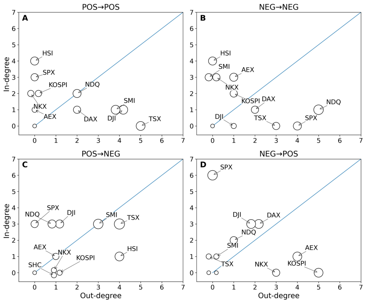
Figure 10 further summarizes these patterns through in-degree and out-degree. In the same-direction abnormal movement relationships, Hong Kong, China, has relatively high in-degree under downward extreme conditions, confirming its receiving role. The U.S. technology-oriented Nasdaq index shows stronger out-degree in the abnormal downward-to-downward relationship, consistent with its outward position in Figure 9. In the abnormal upward-to-upward relationship, Canada is closer to a sending role, while Hong Kong, China, and the United States lean more toward receiving positions. In the opposite-direction relationships, sender and receiver roles become more concentrated. Hong Kong, China, is more outward-oriented in the abnormal upward-to-downward relationship, while the United States has stronger incoming connectivity in the abnormal downward-to-upward relationship.

These results show that the stock index network contains both same-direction abnormal movement relationships and opposite-direction abnormal movement responses. The United States, especially its technology market, plays an important role in transmitting downside tail movements. The broad U.S. market also acts as an important receiving market in some cross-direction relationships, reflecting its position in global capital reallocation. Hong Kong, China, behaves as a downside shock receiver in same-direction relationships and as a more active connector in cross-direction relationships. The Chinese mainland market remains relatively weakly connected, but its link with Hong Kong, China, becomes clearer under certain tail states. Overall, the stock index results suggest that channel-specific tail-triggering networks provide a more detailed view of global equity-market tail risk transmission than a single aggregated stock index network.

5. Conclusions

This paper proposes an outlier-driven framework for reconstructing directed and lagged Tail Outlier-Triggering Networks from financial time series. The simulation experiments show that, compared with CoVaR, a Clayton copula tail-dependent network, and DCC-GARCH, ODNI performs better in reconstructing known ground-truth network structures. Its main advantage lies in its high precision, indicating that the framework can identify relatively reliable tail-triggering links while controlling false positives. The robustness analysis further shows that ODNI performs more stably when the sample length increases and when the true coupling structure becomes more identifiable.

The real-market applications also demonstrate the interpretive value of ODNI. In the foreign exchange market, the inferred networks show a clear regional structure, especially among Asian exchange rate series. In the global stock index market, lower tail outliers are more closely associated with the outward transmission role of the U.S. technology-oriented market, while Hong Kong, China, shows receiver or connector characteristics across different tail channels. These findings suggest that channel-specific tail-triggering networks can reveal asymmetric sender–receiver roles that are difficult to observe in a single aggregated dependence network.

The scope of ODNI is tail outlier transmission. Therefore, it is better understood as a complement to, rather than a substitute for, models of average return dynamics or continuous volatility dependence. However, several limitations remain. First, the framework requires a sufficient number of tail observations; when the sample is short or tail events are too sparse, the estimated triggering probabilities may become unstable. Second, ODNI identifies statistical tail-triggering relationships rather than strict structural causality, so unobserved common shocks and indirect transmission paths may still affect the inferred network. Third, the results may be affected by the selection of tail thresholds, lag orders, and the aggregation rules used to map tail channel links to asset-level networks. Future research may further incorporate adaptive thresholds, multiple lag structures, multivariate attribution mechanisms, and rolling window estimation for dynamic systemic risk monitoring.