Modeling Healthcare Accessibility with Endogenous Search Ranges: A Huff-Based Multi-Source Data Approach

Abstract

This study proposes a Behavior-Calibrated Endogenous Choice 2SFCA (BCEC-2SFCA) framework for assessing spatial accessibility to tertiary hospitals. Using large-scale taxi trajectory data from Ningbo, China, we empirically calibrate the Huff model parameters ($\alpha =1.1758, \beta =2.9608$) based on observed hospital choices and construct travel time and distance matrices from observed trips. Unlike existing Huff-based FCA approaches that assume parameter values, BCEC-2SFCA jointly estimates the attractiveness elasticity and distance-decay coefficient directly from local healthcare travel behavior and integrates these calibrated probabilities into a 2SFCA structure where hospital catchments are endogenously generated rather than exogenously imposed. Compared with conventional Gaussian 2SFCA, the BCEC-2SFCA model produces a continuously varying and behaviorally plausible accessibility surface and better replicates the relative order of hospital attractiveness ($\rho =0.527, p<0.05$), although its RMSE is slightly higher (0.02700 vs. 0.02211) while MAPE is clearly lower (32.17% vs. 42.12%). Robustness checks using all 22 hospitals confirm stable estimates, and subgroup analyses show consistent advantages across hospital scales. The framework is specifically designed for high-order medical services with strong inter-facility competition—such as tertiary hospitals—and its applicability to proximity-based services is limited.

1. Introduction

Spatial accessibility to healthcare services is a central concern in urban planning and public health research, as it directly influences healthcare utilization, equity, and health outcomes. Among different healthcare facility types, tertiary hospitals exhibit distinctive service characteristics: they provide specialized care, attract patients across large spatial ranges, and operate within competitive and hierarchical hospital systems. Accurately capturing accessibility to such facilities therefore requires models that reflect both spatial opportunity structures and residents’ healthcare-seeking behavior.

The Two-Step Floating Catchment Area (2SFCA) method and its variants have become widely used tools for measuring healthcare accessibility due to their intuitive structure and moderate data requirements [1,2,3]. Extensions incorporating distance decay, such as Gaussian or kernel-based 2SFCA models [4,5], have improved realism by allowing service influence to decrease with travel cost. However, these approaches typically rely on exogenously defined catchment thresholds or globally fixed decay parameters [6,7,8], implicitly assuming that residents evaluate healthcare opportunities within uniform spatial or temporal limits.

Such assumptions are problematic in the context of tertiary hospitals. Unlike primary care facilities, tertiary hospitals do not operate within locally bounded catchments; patients often travel well beyond conventional thresholds when perceived service quality or specialization justifies longer journeys. Empirical studies consistently show substantial heterogeneity in healthcare travel behavior across space and population groups, suggesting that fixed catchment definitions are conceptually misaligned with actual decision processes.

To address these limitations, studies have incorporated probabilistic choice models, such as the Huff model [9], into accessibility analysis [10,11]. These approaches allow facilities to compete probabilistically based on attractiveness and distance, thereby capturing the substitution effects among alternative facilities. However, in most existing integrations, probabilistic choice is used only to reweight facility influence, while the effective search range remains externally imposed or implicitly constrained. As a result, the fundamental question of how far residents are behaviorally willing to search remains unresolved.

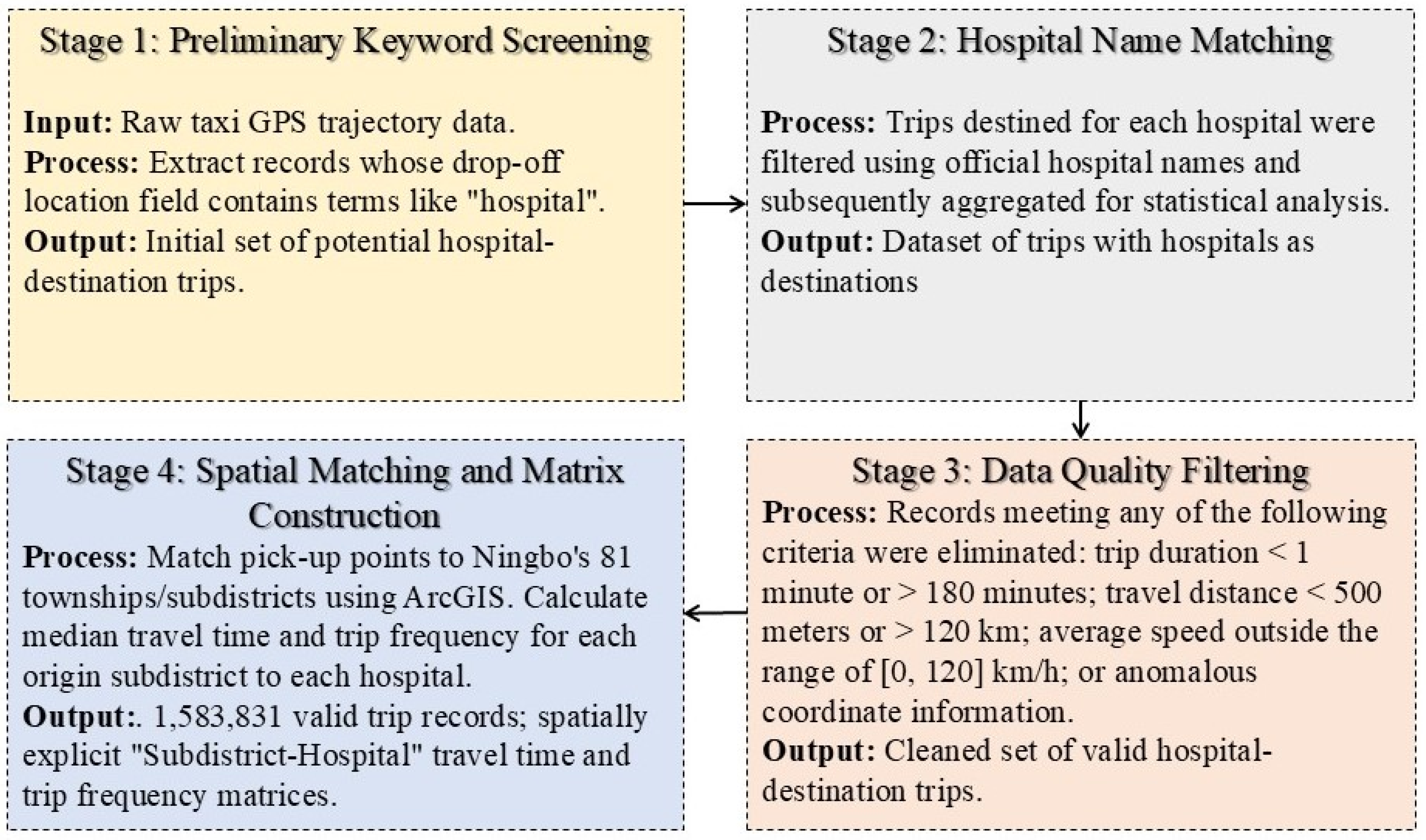
This study argues that accessibility assessment should be grounded in observed travel behavior rather than arbitrary thresholds. To achieve this, we leverage large-scale taxi trajectory data to empirically calibrate the Huff model parameters from observed hospital choices and to construct realistic travel impedance matrices from actual trips.

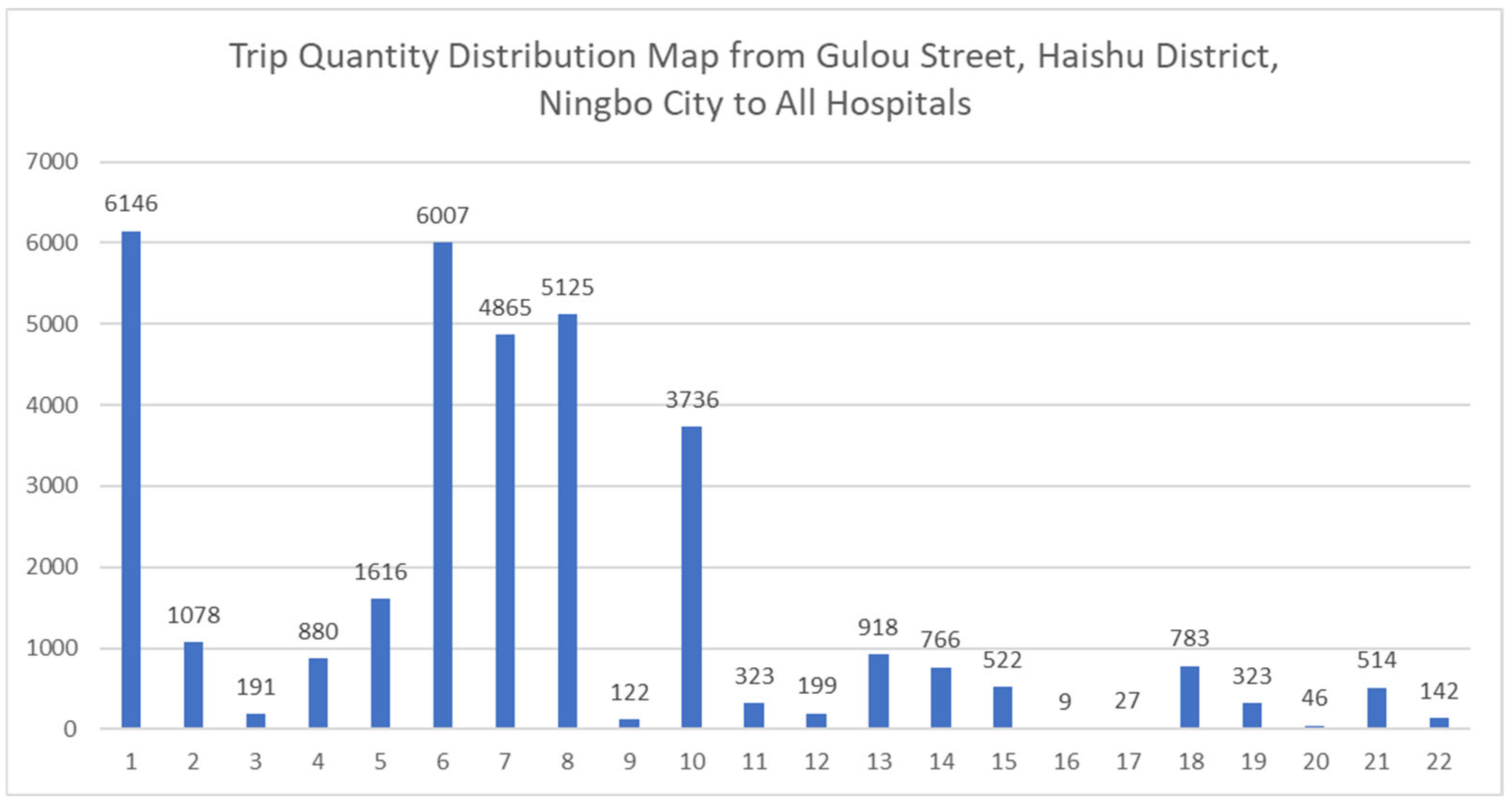
Taxi data capture actual road-network conditions, including congestion and route choices. We construct a complete origin–destination travel time matrix between all residential townships/subdistricts and tertiary hospitals based on observed taxi trips. Building on these data-driven foundations, we propose a Behavior-Calibrated Endogenous Choice 2SFCA (BCEC-2SFCA) framework. The model supplies origin-specific choice probabilities that reflect competition among hospitals, calibrated from observed taxi trips, while the 2SFCA structure accounts for supply–demand ratios and cumulative opportunities without imposing exogenous catchment thresholds. The resulting accessibility measure captures both the attractiveness of hospitals and the actual travel burden experienced by residents, without imposing exogenous catchment thresholds.

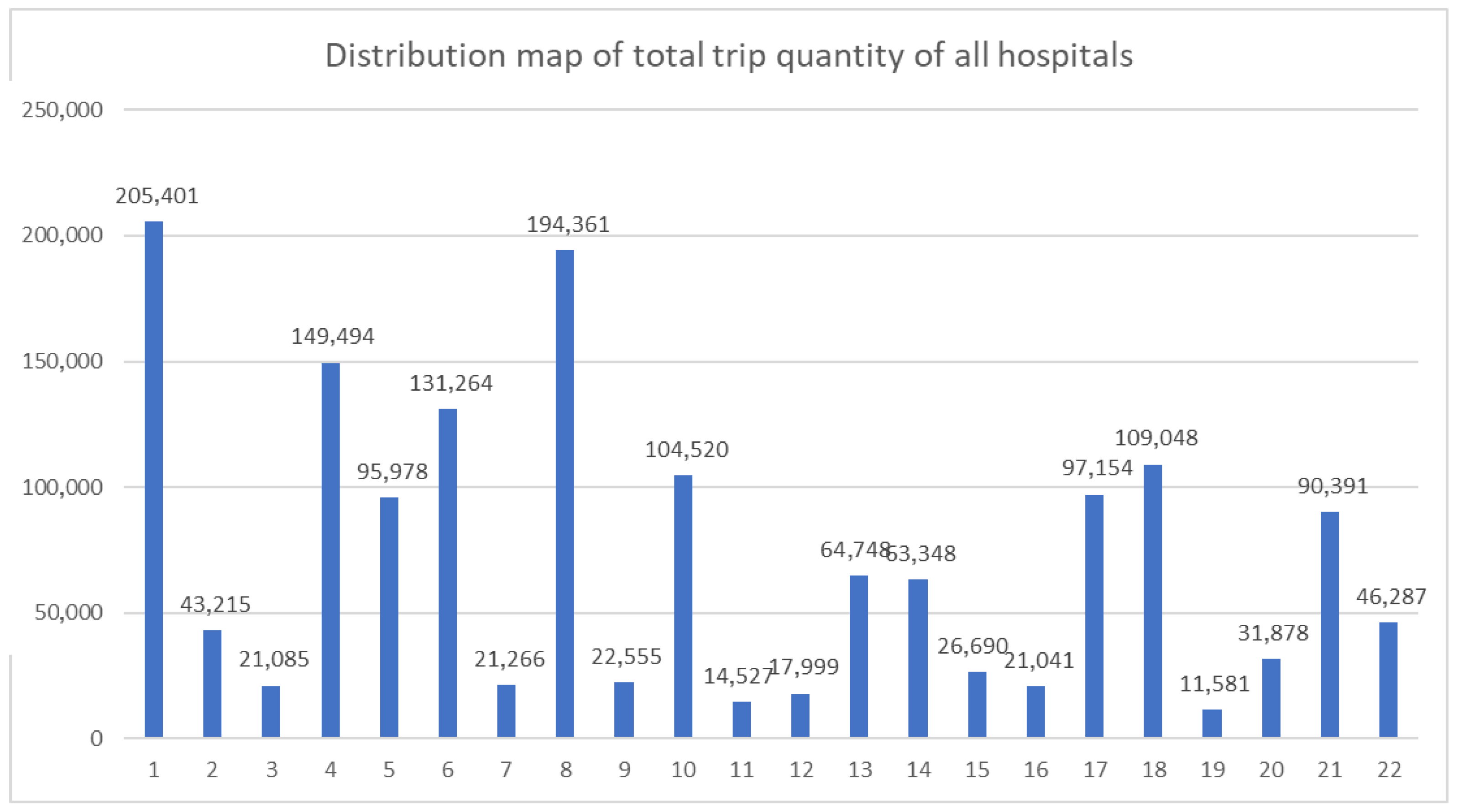
The proposed framework is empirically validated using multi-source data from Ningbo, China: hospital bed capacity, township-level population, over 1.58 million taxi trajectories, and annual outpatient volumes from 16 tertiary hospitals. By comparing modeled accessibility outcomes with observed travel patterns and outpatient distributions, we provide behavioral evidence for the validity of our approach.

This study makes three main contributions: (1) empirical calibration of Huff model parameters from observed taxi trips; (2) construction of high-resolution travel impedance matrices from real-world trajectories; and (3) integration of these elements into a behavior-calibrated 2SFCA framework (BCEC-2SFCA) that generates endogenous search ranges.

It is important to emphasize that the proposed framework is specifically designed for high-order medical services—namely tertiary hospitals—which are characterized by strong inter-facility competition, large service areas, and prevalent cross-regional healthcare-seeking behavior. The endogenous search range mechanism is predicated on the assumption that patients actively compare and choose among multiple alternative facilities, a condition that does not hold for proximity-based services such as community health centers, where travel is typically constrained to a local catchment. The applicability of the BCEC-2SFCA model to primary care or other locally bounded service contexts should therefore be considered limited, and the conventional Gaussian 2SFCA or similar threshold-based methods may remain more appropriate in those settings.

2. Literature Review

Accessibility is a crucial concept for estimating the ease with which people can overcome spatial barriers to access services or resources. W. G. Hansen first defined it in 1959 as “the potential of opportunities for interaction,” laying the foundation for accessibility research [12]. Since then, the concept has expanded to encompass transportation, temporal, and psychological dimensions, becoming a core metric in geography and urban planning [13].

Current methods for measuring healthcare resource accessibility primarily include the cumulative opportunity measure [14], distance-based measure, network analysis [15], isochrone method [16], gravity model, and the two-step floating catchment area (2SFCA) method [17]. These approaches have evolved by incorporating more realistic factors to enhance their explanatory power [18].

The minimum distance method [19] and buffer analysis evaluate accessibility by calculating the straight-line distance to the nearest facility or setting a fixed service radius. These methods are simple and intuitive, often used for preliminary delineation of hospital service areas. However, neither considers the constraints of the actual transportation network, which may lead to discrepancies with real-world conditions.

Network analyses can answer a range of questions related to linear networks such as roads, railways, rivers, facilities and utilities. This spatial analysis technique uses network data (usually linear features such as roads, footpaths) to calculate distances between points or nodes on the network. This approach underpins the satellite navigation systems found in many cars. Common applications are route finding, route planning, identifying the closest facility by travel time or distance, calculation of service areas (e.g., areas within 10 min’s walk of a bus stop), etc. There are various ways of parameterising the analysis based on typical road speeds, blockages, and minimising the use of smaller or remote parts of the network depending on the task [20].

The gravity model is one of the most representative and classic methods in spatial interaction and accessibility analysis. Originating from Newton’s law of universal gravitation, it was first introduced into human geography and transportation planning by Zipf [21,22], and later endowed with a rigorous statistical mechanics foundation by Wilson within the framework of entropy maximization, thereby evolving from an empirical formula into a systematic theory of spatial interaction [23]. In accessibility research, the fundamental principle of the gravity model is that the intensity of interaction between two locations (e.g., trip volume) is proportional to the “mass” of the origin (e.g., population size) and the “mass” of the destination (e.g., facility service capacity), and inversely proportional to a power of the spatial impedance (distance or time) between them. When applied to measure accessibility, the model is often used in its “potential model” form, which sums the service capacities of all medical facilities j weighted by a distance decay function for a given residential location i, thereby yielding a continuous accessibility score for that location. Compared with the cumulative opportunity method or the isochrone method, the gravity model offers the advantage of incorporating continuous distance decay, thus avoiding the issue of threshold discontinuity. In contrast to the two-step floating catchment area method, its traditional form typically does not explicitly address competition effects on the demand side. The two-step floating catchment area (2SFCA) method was first proposed by Radke and Mu (2000) [17], and the version modified by Luo and Wang (2003) [1] has been widely used. The 2SFCA method fully considers the influence of both supply-side and demand-side scales on accessibility and has become a primary research method for measuring spatial accessibility in the healthcare field. Extensions of the 2SFCA method by researchers can be summarized into four categories: (1) extensions of the distance decay function, (2) extensions of the catchment radius, (3) mode-of-transport-based extensions, and (4) extensions targeting demand or supply. The distance decay functions commonly used by researchers include a piecewise decay form that assigns different weights to different travel time intervals within the catchment area [24], the gravity decay model, the kernel density form [5], and the Gaussian form [4].

Luo et al. proposed an enhanced two-step floating catchment area (E2SFCA) method to address the assumption of uniform accessibility within the catchment area in the traditional 2SFCA method. This method assigns differentiated weights to different travel time intervals in both steps to reflect the distance decay effect [24]. The gravity-based 2SFCA method introduces the distance decay function from the well-established gravity model into the 2SFCA framework, thereby improving the discrete distance decay function of the E2SFCA method into a continuous function. The kernel density 2SFCA (KD2SFCA) method, proposed by Dai [5], incorporates a kernel density-based distance decay function within the 2SFCA catchment radius. The kernel density decay function is concave: when the distance is small, accessibility decays slowly with increasing distance; as the distance increases, the decay accelerates. Based on the 2SFCA method, Dai introduced a Gaussian function to continuously weight the distance decay within the catchment area and formally proposed the Gaussian 2SFCA method. Using the Detroit metropolitan area as the study region, Dai investigated the impact of racial residential segregation and spatial accessibility to healthcare facilities on the rate of late-stage breast cancer diagnosis, aiming to more accurately assess the spatial accessibility of medical facilities [4].

After its introduction, the 2SFCA method rapidly became one of the most widely recognized and commonly used approaches in healthcare accessibility research. Numerous subsequent studies have employed the 2SFCA method or its improved versions for accessibility assessment. Ahmed et al. used walking time and the 2SFCA method to evaluate accessibility to cyclone shelters in the coastal region of Bangladesh, and applied the Gini coefficient to analyze interregional inequalities [25]. Cheng et al. took Nanjing, China as the study area, used the 2SFCA method to assess the spatial accessibility of multi-level hospital services for the elderly, and employed the Gini coefficient to examine spatial equity in accessibility [26]. Mao et al. incorporated multiple different transportation modes into the mobile two-step floating catchment area method and compared it with the traditional single-mode two-step floating catchment area method. They found that the accessibility calculated using multi-modal transportation technology held more practical significance than results from single-mode calculations [27]. Qu et al. systematically evaluated the influence of spatial resolution selection on measurement errors in public transit accessibility, using Melbourne, Australia as the study area. They selected representative points at different resolutions, calculated three accessibility metrics—proximity, cumulative opportunity, and Gaussian 2SFCA—and compared the measurement errors against building-level benchmark data [28]. Juel et al., considering that travel time to medical facilities varies according to specific daily conditions, used an improved two-step floating catchment area method to evaluate the accessibility of public healthcare services in developing countries in the Caribbean region. They proposed that increasing the allocation of physicians could improve the accessibility of medical facilities [29].

In addition, some scholars have incorporated competitive relationships into the 2SFCA framework to improve the method. Jin et al. proposed a 2SFCA approach integrating multiple transportation modes (driving, transit, and walking) with the Huff choice model to assess spatial accessibility to healthy and unhealthy food stores in Austin, Texas, USA, revealing significant disparities between the urban core and peripheral areas [30]. Subal et al. improved the Huff 3SFCA method by replacing discrete zone-based weights with a continuous Gaussian distance-decay function to quantify the spatial accessibility of general practitioners in the Swabian region of Germany, identifying accessibility differences between urban and rural areas as well as within cities at the micro-scale [31]. Mo et al. employed a Huff-model-based 2SFCA method to evaluate the accessibility of community care services in Hong Kong [32]. Zhu et al. conducted a study in Luyang District, Hefei City, China, where they integrated the Gaussian distance-decay function and the Huff model into the traditional 2SFCA framework, while also considering two low-carbon travel modes (walking and public transit) to evaluate the accessibility of meal service facilities for the elderly [33]. Chen et al. proposed a generalized flow-based 2SFCA method using Wuhan City as a case study. They extracted residents’ origin–destination flows for healthcare visits from taxi trajectory data, adaptively determining the catchment area, distance-decay coefficient, and attractiveness for each hospital. On this basis, they constructed a global popularity index based on the h-index concept and a local preference index reflecting community-level healthcare preferences, and incorporated these indices into the Huff model for accessibility assessment [34].

While the integration of Huff models into accessibility analysis has gained increasing attention, the calibration of Huff model parameters—the attractiveness elasticity α and the distance-decay coefficient β—remains a critical challenge. In most existing Huff-FCA studies, these parameters are either assumed based on prior literature (e.g., α = 1, β = 2) or determined through ad hoc sensitivity tests. However, because α and β govern the sensitivity of residents to facility attractiveness and travel impedance, respectively, arbitrarily setting their values risks producing accessibility estimates that deviate systematically from actual travel behavior.

Recognizing this limitation, a growing body of research has sought to calibrate Huff model parameters using observed behavioral or location-based data, moving beyond assumed parameter values toward empirically grounded estimates. Yue et al. were the first to use taxi GPS trajectory data as a substitute for traditional questionnaire surveys to conduct an exploratory calibration of the Huff model, thereby demonstrating the feasibility of using large-scale trajectory data for retail trade area analysis [35]. Gong et al. proposed using geographically and temporally weighted regression (GTWR) to simultaneously calibrate spatial and temporal parameter variations in the Huff model, revealing that attractiveness sensitivity is positively correlated with residents’ wealth and negatively correlated with leisure time [36]. Gong et al. also developed an agent-based Destination-Aware Activity Simulation (DAS) model, incorporating geographically weighted regression (GWR) to calibrate agents’ destination choice parameters, enabling the dynamic simulation of residents’ multi-activity sequences [37]. Liang et al. proposed a time-aware dynamic Huff model (T-Huff), employing large-scale mobile phone location data and particle swarm optimization to characterize the time-varying patterns of market shares across different business formats [38]. Lu et al. investigated the influence of the number of sampling points on the calibration accuracy of the Huff model using mobile phone location data, finding that a small number of sampling points with high trip volumes can yield better calibration performance [39].

In summary, three critical gaps in the existing Huff-based FCA literature are identified and addressed in this work. First, Huff parameters are typically assumed rather than empirically calibrated from local healthcare travel data. Second, impedance matrices are usually derived from idealized distances, failing to capture real-world travel conditions. Third, even with Huff probabilities, the effective service range remains constrained by exogenously imposed thresholds. This study addresses these gaps by integrating empirically calibrated Huff choice probabilities—derived from large-scale taxi trajectory data—into a 2SFCA framework to generate endogenous hospital search ranges, thereby eliminating reliance on both assumed behavioral parameters and exogenously imposed catchment thresholds. More precisely, the proposed BCEC-2SFCA framework makes three distinct contributions: (1) joint empirical calibration of α and β from observed taxi trips; (2) construction of an impedance matrix from actual travel times; and (3) a probabilistic 2SFCA structure in which catchment areas are endogenously generated by choice probabilities. The following section details the data and methods that operationalize this framework.

3. Methodology

3.1. Overview of the Framework

This study develops a Behavior-Calibrated Endogenous Choice 2SFCA (BCEC-2SFCA) framework for tertiary hospitals by integrating a Huff-type probabilistic choice model with the supply–demand logic of the two-step floating catchment area (2SFCA) method. The framework is designed to replace exogenously specified service catchments with an endogenously generated search range, inferred from observed travel behavior, hospital attractiveness, and inter-hospital competition.

The methodological workflow consists of three components. First, hospital-oriented taxi trajectories are used to construct an empirical origin–destination impedance matrix based on observed travel time and travel distance. Second, the parameters of a Huff choice model are calibrated from revealed destination choices so that the probability of selecting each hospital reflects the joint effects of hospital attractiveness and travel impedance. Third, the estimated choice probabilities are embedded into a probabilistic 2SFCA structure to compute hospital-specific supply–demand ratios and origin-specific accessibility scores.

The conceptual difference from conventional 2SFCA is important. In standard Gaussian 2SFCA models, the analyst predefines the effective service range using a fixed threshold or a globally imposed decay function. In the proposed framework, by contrast, the effective service range is not fixed a priori. Instead, it emerges from the estimated choice probabilities across all hospitals. A hospital with stronger attractiveness or weaker competitive pressure can exert influence over a wider area, whereas a less attractive hospital faces a narrower effective reach. Therefore, the search range is treated as endogenous to the healthcare system, rather than externally imposed.

This section presents the theoretical specification of the BCEC-2SFCA framework, including the Huff probabilistic choice model, the derivation of endogenous search ranges, and the two-step accessibility formulation. The empirical implementation—data sources, matrix construction, and parameter calibration—is detailed separately in Section 4.

3.2. Endogenous Search Range Through Probabilistic Hospital Choice

3.2.1. Hospital Choice Model Based on Calibrated Huff-Type Probabilities

Residents’ choice of tertiary hospitals is modeled using a Huff-type probabilistic formulation:

$$P_{ij}={\displaystyle \frac{S_j^{\alpha }\cdot c_{ij}^{-\beta }}{{\displaystyle {\sum }_{k=1}^m} S_k^{\alpha }\cdot c_{ik}^{-\beta }}}$$

(1)

where:

i = 1, 2, …, n denote demand locations, represented by townships/subdistricts;

j = 1, 2, …, m denote tertiary hospitals;

$P_{ij}$ is the choice probability of the resident at demand point i for hospital j;

$S_j$ is the supply capacity of hospital j;

$c_{ij}$ is the travel impedance from demand point i to hospital j, measured by observed travel time or travel distance;

$\alpha$ is the service-capacity elasticity parameter;

$\beta$ is the impedance-decay parameter;

${\displaystyle {\sum }_{k=1}^m}$ denotes the summation over the supply capacity of all alternative tertiary hospitals.

Equation (1) implies that the probability of choosing a hospital increases with hospital attractiveness and decreases with travel impedance. More importantly, it is normalized over all competing hospitals, so the attractiveness of any hospital is always evaluated relative to the alternatives available to the same origin. This allows inter-hospital competition to be represented directly within the accessibility model.

The term “endogenous search range” can now be defined rigorously. For any demand location i, the effective set of hospitals $Ri\left(\tau \right)$ considered by residents is not determined by a fixed threshold such as 30 min or 20 km. Instead, it is generated by the set of hospitals with non-negligible choice probabilities:

$$Ri\left(\tau \right)=\{j\mid P_{ij}\ge \tau \}$$

(2)

where $\tau$ is a small behavioral relevance threshold. Under this definition, the search range varies across origins and hospitals according to the joint effects of attractiveness, impedance, and competition. Thus, range is an outcome of the model rather than an external assumption.

3.2.2. Parameter Calibration from Observed Trips

To avoid imposing arbitrary parameter values, α and β are calibrated using observed hospital-oriented taxi trips. Let $N_{ij}$ denote the number of observed taxi trips from demand location i to hospital j, and let the observed hospital choice share be:

$$P_{ij}^{\mathrm{o}\mathrm{b}\mathrm{s}}={\displaystyle \frac{N_{ij}}{{\displaystyle {\sum }_{k=1}^m} N_{ik}}}$$

(3)

The Huff parameters are estimated by fitting the modeled choice probabilities $P_{ij}$ in Equation (1) to the observed shares $P_{ij}^{obs}$. This can be implemented using Log-centered transformation and Ordinary Least Squares (OLS) on the origin-hospital observations (See Section 4.2 for details).

The estimated parameters quantify two distinct behavioral mechanisms:

α captures the sensitivity of residents to hospital capacity, while β measures how quickly hospital attractiveness declines with increasing travel impedance. Because these parameters are estimated from observed mobility rather than borrowed from previous studies, the accessibility model becomes more behaviorally grounded and more context-specific.

3.3. Construction of the Empirical Impedance Matrix

The spatial impedance matrix is built from taxi trajectory data linking demand locations to tertiary hospitals. For each observed origin-hospital pair, travel time and travel distance are extracted from actual taxi trips. These observations reflect real road-network conditions, including congestion, route choice, and temporal variation, thereby providing a more realistic measure of healthcare-related travel cost than Euclidean distance or idealized network paths. The impedance matrix is constructed solely from observed taxi trips, providing complete coverage for all OD pairs.

3.4. Probabilistic 2SFCA Accessibility Model

The calibrated choice probabilities are then incorporated into a probabilistic 2SFCA framework.

3.4.1. Step 1: Hospital Supply–Demand Ratio

For each hospital j, the expected demand is defined as the population-weighted sum of origin-specific hospital choice probabilities:

$${\tilde{D}}_j={\displaystyle \sum _{i=1}^n} D_i{P}_{ij}$$

(4)

where $D_i$ denote the population at demand location i. This expression replaces the conventional fixed-catchment demand aggregation. In standard 2SFCA, only demand within a predefined threshold contributes to hospital congestion. Here, all demand locations may contribute, but their contributions are weighted by the estimated probability of choosing that hospital. Consequently, the effective catchment of each hospital becomes behavior-dependent and hospital-specific.

The effective supply–demand ratio of hospital j is then given by:

$$R_j={\displaystyle \frac{S_j}{{\tilde{D}}_j}}={\displaystyle \frac{S_j}{{\displaystyle {\sum }_{i=1}^n} D_i{P}_{ij}}}$$

(5)

A higher $R_j$ indicates that hospital j has greater effective service capacity relative to the demand it is expected to attract.

3.4.2. Step 2: Accessibility at Each Demand Location

The accessibility of origin i is defined as the expected supply–demand ratio across all hospitals, weighted by the hospital choice probabilities:

$$A_i={\displaystyle \sum _{j=1}^m} P_{ij}{R}_j$$

(6)

Substituting Equation (5) into Equation (6) yields:

$$A_i={\displaystyle \sum _{j=1}^m} P_{ij}{\displaystyle \frac{S_j}{{\displaystyle {\sum }_{i=1}^n} D_i{P}_{ij}}}$$

(7)

Equation (7) is the core accessibility measure used in this study. It retains the two-step logic of 2SFCA by accounting for both hospital congestion and demand-side access, but it eliminates the need for externally imposed catchment thresholds. Accessibility is instead determined by the endogenous hospital choice structure estimated from observed travel behavior.

3.5. Interpretation of the Endogenous Search Range

Under the proposed model, the effective influence range $Ri\left(\tau \right)$ of a hospital is not fixed across space. For a large and attractive hospital, the term $S_j^{\alpha }$ may offset higher travel impedance, allowing the hospital to retain meaningful choice probabilities over a wider area. Conversely, smaller or less attractive hospitals may have influence concentrated in nearby locations only. Likewise, for residents in peripheral areas with few competitive options, the dominant hospital may exhibit a broader effective search range than for residents in central areas with many alternatives.

Therefore, the endogenous search range is not represented by a single citywide threshold. Instead, it is embedded in the probability surface {Pij}, which varies across origins and facilities and is jointly shaped by attractiveness, impedance, and competition.

To provide a more intuitive geographical interpretation, the endogenous search range can be likened to a “probability cloud” surrounding each hospital, rather than a sharply bounded circle. In conventional threshold-based models, a hospital is either inside or outside a resident’s search range depending on whether the travel cost falls below a fixed cutoff—a binary, all-or-nothing designation. In the BCEC-2SFCA framework, by contrast, every hospital exerts some degree of influence on every origin, but the strength of that influence decays continuously with travel impedance and is further modulated by the hospital’s attractiveness relative to its competitors. A hospital with high attractiveness (e.g., a large tertiary center) may retain a non-negligible choice probability even for residents located 50 km away, meaning that it remains part of their effective search range. Conversely, a smaller hospital may fade into the background of the probability surface beyond a much shorter distance. The effective search range is therefore not a predefined geometric shape but an emergent property of the spatial pattern of choice probabilities—a gradient that captures both the friction of distance and the pull of service quality. This probabilistic, gradient-based conception of search range aligns more closely with the continuous nature of human spatial behavior than do conventional hard thresholds.

3.6. Standardization and Spatial Comparison

To facilitate spatial visualization and comparison across townships/subdistricts, the raw accessibility values Ai are standardized using max-normalization:

$$A_i^{\ast }={\displaystyle \frac{A_i}{{max}_i A_i}}$$

(8)

where $A_i^{\ast }$∈(0,1]. Higher values indicate better relative access to tertiary hospital services.

3.7. Benchmark Model: Gaussian 2SFCA

To evaluate the effect of the proposed endogenous-range framework, its results are compared with those of a conventional Gaussian 2SFCA model. In the benchmark model, we use travel time as impedance, hospital supply–demand ratios are calculated using a predefined travel threshold and a Gaussian decay function:

Step 1:

$$R_j^G={\displaystyle \frac{S_j}{\sum _{i:t_{ij}⩽t_0} D_i{G(t}_{ij},t_0)}}$$

(9)

where $d_0$ is the fixed catchment threshold and $f\left(d_{ij}\right)$ is the Gaussian decay function.

$${G(t}_{ij},t_0)=\left\{\begin{array}{cc}{\displaystyle \frac{{\mathrm{e}}^{-\frac{1}{2}\times {\left(\frac{t_{ij}}{t_0}\right)}^2}-{\mathrm{e}}^{-\frac{1}{2}}}{1-{\mathrm{e}}^{-\frac{1}{2}}}}\hfill & t_{ij}⩽t_0\hfill \\ 0\hfill & t_{ij}>t_0\hfill \end{array}\right.$$

(10)

Step 2:

$$A_i^G=\sum _{j:t_{ij}⩽t_0} R_j^G{G(t}_{ij},t_0)$$

(11)

Unlike the proposed model, this benchmark relies on exogenously defined spatial influence. The comparison therefore highlights the extent to which behavior-calibrated, endogenous search ranges alter the resulting accessibility pattern.

3.8. Methodological Contribution

The proposed method contributes to accessibility assessment in three ways. First, it estimates hospital choice sensitivities from observed trips rather than assuming parameter values. Second, it constructs the impedance matrix from real trajectory data rather than idealized distances. Third, it embeds these empirically estimated choice probabilities into a supply–demand accessibility framework—the BCEC-2SFCA—in which the effective hospital search range is generated endogenously. The resulting model is particularly suitable for tertiary hospital systems characterized by long-distance patient movement, strong facility competition, and heterogeneous travel behavior.

4. Data and Implementation

4.1. Data Processing and Initial Matrix Construction

Building on the theoretical framework presented in Section 3, this section describes the empirical implementation of the BCEC-2SFCA model. To implement the proposed model, this section details the research data and its processing workflow. The core objective is to construct four spatial impedance matrices for model calculation and parameter calibration: the trip frequency matrix $N_{obs}$, the observed choice probability matrix $P_{obs}$, the median travel time matrix $T_{obs}$, and the median travel distance matrix $D_{obs}$. The empirical analysis of this study is based on multifaceted data from Ningbo City, China.

4.1.1. Definition of the Study Area

This study focuses on the principal urban area of Ningbo, encompassing the districts of Haishu, Jiangbei, Yinzhou, Zhenhai, Beilun, and Fenghua (Figure 1). The primary consideration for selecting this area as the research scope is that it concentrates the vast majority of tertiary hospital resources in Ningbo, where residents’ healthcare travel behavior is intensive and exhibits typical patterns, effectively reflecting the service characteristics of tertiary hospitals. Ninghai County, Xiangshan County, Cixi City, Yuyao City, and the hospitals within their jurisdictions are temporarily excluded from this study due to their considerable distance from the main urban area and the fact that their healthcare travel patterns exhibit significant differences.

The six districts included in the study area have a combined permanent population of approximately 5.33 million as of 2024, with population densities varying considerably from the densely populated urban core (e.g., Haishu and Yinzhou) to the more sparsely populated peripheral districts (e.g., Fenghua and Beilun). The 22 tertiary hospitals in the study area collectively provide over 20,000 inpatient beds, with bed counts per hospital ranging from approximately 150 to 1900. The average road distance between a township/subdistrict centroid and its nearest tertiary hospital is approximately 9 km, while the distance to the nearest hospital exceeds 30 km in some peripheral areas, underscoring the substantial spatial variation in healthcare access across the region.

4.1.2. Data Sources and Preprocessing

Two primary categories of data are used: taxi trajectory data and hospital attribute data.

(1)

Taxi Trajectory Data: The dataset covers trips within Ningbo from 1 March to 30 November 2023. Each record includes timestamps, longitude/latitude coordinates for pick-up and drop-off locations, travel distance, and calculated trip duration.

(2)

Hospital Data: Geographic locations (longitude/latitude) and service capacity metrics were collected for all tertiary hospitals in study area. The number of available beds for each hospital serves as the proxy variable for its supply capacity $S_j$.

Data processing aimed to identify and extract valid trips with hospitals as destinations suitable for travel behavior analysis. The workflow is illustrated in Figure 2. Key steps include:

1.

Preliminary Screening:

From the raw data, all records containing terms such as “hospital” in the drop-off location field were extracted.

2.

Hospital Name Matching:

Trips with drop-off locations corresponding to each specific hospital (e.g., “The Affiliated First Hospital of Ningbo University”) were extracted based on the hospital name and then aggregated for statistical analysis.

3.

Data Cleaning:

To eliminate recording errors and exceptional cases, trips meeting any of the following criteria were removed:

(a)

trips with a travel time of less than 1 min or greater than 180 min;

(b)

trips with a travel distance of less than 500 m or greater than 120 km;

The time and distance thresholds serve to exclude recording errors and data noise: the lower bounds (1 min, 500 m) remove likely mis-recorded drop-offs and short-distance positioning errors, while the upper bounds (180 min, 120 km) are set generously to retain legitimate long-distance healthcare-seeking trips—a defining characteristic of tertiary hospital access. Notably, only 0.03% of candidate trips exceeded 120 km, and only 0.32% were shorter than 500 m.

(c)

trips with an average speed outside the range of [5,100] km/h, to exclude trips with speeds clearly deviating from the typical range of urban road traffic;

(d)

trips with clearly anomalous coordinate information, to exclude cross-city trips and obvious GPS anomalies.

4.

Demand Point Administrative Division Matching:

For spatial analysis, the 81 townships/subdistricts of Ningbo were used as demand units, with the centroid of each township/subdistrict representing a demand point i. Using ArcGIS spatial analysis tools (ArcGIS 10.8, Esri, Redlands, CA, USA), the pick-up point of each trip was matched to the township/subdistrict polygon in which it was located. These 81 townships and subdistricts constitute the finest administrative divisions within the six districts and serve as the demand units (i = 1, 2, …, 81) throughout the subsequent accessibility analysis.

This process yielded 1,583,831 valid trip records, forming the foundation for subsequent analysis.

Figure 3 presents the distribution of taxi visit volumes to different hospitals. The black box in the figure indicates the central urban area of Ningbo, and each red circle represents a hospital. The larger the red circle, the greater the taxi visit volume to that hospital during the study period. As can be seen from the figure, most tertiary hospitals are concentrated in the central urban area, and the taxi visit volumes of these centrally located hospitals are generally high. In contrast, hospitals in peripheral areas (e.g., Zhenhai District, Jiangbei District, and Fenghua District) have relatively lower taxi visit volumes. It should be noted that this figure presents raw data on taxi visit intensity derived from trajectory data, which is a distinct concept from hospital annual outpatient volume. The relationship between taxi visit volume and outpatient volume isfurther analyzed later (see the subsection “Selection of Hospitals for Parameter Calibration” in Section 4.2.2), where a subset of hospitals exhibiting a strong linear correspondence with outpatient volume is identified for model calibration.

Figure 4 shows significant differences in taxi visit volumes across hospitals. The visit volume of The First Affiliated Hospital of Ningbo University is considerably higher than that of specialized institutions such as Ningbo Kangning Hospital. Moreover, taxi visits to each hospital are mainly concentrated in areas close to the hospital.

Figure 5 and Figure 6 present the distribution of trip volumes from Gulou Subdistrict in Haishu District to each hospital and the distribution of total trip volumes for all hospitals, respectively. Both figures clearly illustrate the variations in taxi visit volumes among the different hospitals.

4.1.3. Initial Spatiotemporal Matrices

Based on the cleaned data, four key matrices were constructed as the basis for parameter calibration and model computation:

1.

Trip Count Matrix ($N_{\mathrm{o}\mathrm{b}\mathrm{s}}$):

The total number of trips $N_{ij}$ during the observation period was counted for each “subdistrict i—hospital j” pair, forming a 81 × 22 matrix.

2.

Observed Choice Probability Matrix ($P_{\mathrm{o}\mathrm{b}\mathrm{s}}$):

To transform trip counts into a probabilistic representation of residents’ choice behavior, the observed choice probability was calculated based on the trip count matrix. For each subdistrict i, the observed probability of choosing hospital j is calculated as:

$$P_{ij}^{\mathrm{o}\mathrm{b}\mathrm{s}}={\displaystyle \frac{N_{ij}}{{\displaystyle {\sum }_{k=1}^{22}} N_{ik}}}$$

(12)

$P_{ij}^{\mathrm{o}\mathrm{b}\mathrm{s}}$ satisfies ${\displaystyle {\sum }_{j=1}^{22}} P_{ij}^{\mathrm{o}\mathrm{b}\mathrm{s}}=1$, representing the total probability of choice across all hospitals for residents in that subdistrict. This matrix directly reflects the spatial pattern of residents’ healthcare destination choices.

3.

Median Travel Time Matrix ($T_{\mathrm{o}\mathrm{b}\mathrm{s}}$):

For each subdistrict i and hospital j, the median travel time of all trips is calculated, forming a complete 81 × 22 matrix $T_{obs}$.

4.

Median Travel Distance Matrix ($D_{\mathrm{o}\mathrm{b}\mathrm{s}}$):

For each subdistrict i and hospital j, the median travel distance of all trips is calculated, forming a complete 81 × 22 matrix $D_{\mathrm{o}\mathrm{b}\mathrm{s}}$.

Preliminary analysis of the trip duration matrix revealed three important features:

(1)

Spatial Coverage Characteristics of the Data: the dataset provides complete coverage: for every township/subdistrict and hospital pair, observed taxi trips are available, ensuring a full origin–destination matrix.

(2)

Travel Time Distribution Characteristics: The median travel time for all valid OD pairs ranges from 3.9 to 110.5 min, with a mean of 33.2 min. Travel time interval analysis shows that the 15–30 min interval accounts for the highest proportion (31.1%), followed by the 30–45 min (29.2%) and 45–60 min (19.5%) intervals. This distribution aligns with the characteristic of tertiary hospitals serving large areas and involving medium-to-long-distance travel.

(3)

Travel Distance Distribution Characteristics: The median travel distance for all valid OD pairs ranges from 1.4 km to 87.4 km, with a mean of 22.6 km. Travel distance interval analysis shows that the 10–20 km interval accounts for the highest proportion (26.2%), followed by the 0–10 km (25.5%) and 20–30 km (18.1%) intervals. This distribution also aligns with the characteristic of tertiary hospitals serving large areas and involving medium-to-long-distance travel.

4.2. Behavioral Parameter Calibration

4.2.1. Theoretical Derivation: Log-Centering Transformation of the Huff Model

To calibrate the service capacity elasticity coefficient α and the impedance decay coefficient β in the Huff model, this study follows the classic approach of Yang et al. (2012) [35], adopting the log-centering transformation proposed by Nakanishi and Cooper (1982) [40] to convert the nonlinear Huff model into a linear estimable form, and then using Ordinary Least Squares (OLS) for parameter estimation. It should be noted that this calibration is performed exclusively using travel time impedance; the resulting parameters ($\alpha =1.1758, \beta =2.9608$) capture residents’ actual sensitivity to time cost. In the subsequent BCEC-2SFCA model based on travel distance, these same parameters are retained to maintain behavioral consistency, thereby focusing the comparison on the sensitivity of accessibility outcomes to different impedance specifications.

For each demand point $i$ and hospital $j$, the standard Huff model is expressed as:

$$P_{ij}={\displaystyle \frac{S_j^{\alpha }\cdot t_{ij}^{-\beta }}{{\displaystyle {\sum }_{k=1}^m} S_k^{\alpha }\cdot t_{ik}^{-\beta }}}$$

(13)

where $P_{ij}$ represents the theoretical probability of choosing hospital $j$ from demand point $i$, $S_j$ is hospital service capacity, $t_{ij}$ is the healthcare travel time from $i$ to $j$, α and β are parameters to be estimated.

Taking the natural logarithm of both sides and separating the denominator gives:

$$\ln \left(P_{ij}\right)=\alpha \ln \left(S_j\right)-\beta \ln \left(t_{ij}\right)-C_i$$

(14)

where $C_i=\ln \left({\displaystyle {\sum }_{k=1}^m} S_k^{\alpha }\cdot t_{ik}^{-\beta }\right)$ is an origin-specific constant.

To eliminate $C_i$, we compute geometric means over all hospitals j for each origin i:

$${\tilde{P}}_i={\left({\displaystyle \prod _{j=1}^m} P_{ij}\right)}^{{\displaystyle \frac{1}{m}}},{\tilde{S}}_i={\left({\displaystyle \prod _{j=1}^m} S_j\right)}^{{\displaystyle \frac{1}{m}}},{\tilde{t}}_i={\left({\displaystyle \prod _{j=1}^m} t_{ij}\right)}^{{\displaystyle \frac{1}{m}}}$$

Applying the same logarithmic transformation to these geometric means yields:

$$\mathrm{l}\mathrm{n}\left({\tilde{P}}_i\right)=\alpha \mathrm{l}\mathrm{n}\left({\tilde{S}}_i\right)-\beta \mathrm{l}\mathrm{n}\left({\tilde{t}}_i\right)-C_i$$

(15)

Subtracting (15) from (14) eliminates the origin-specific constant $C_i$:

$$\ln \left({\displaystyle \frac{P_{ij}}{{\tilde{P}}_i}}\right)=\alpha \ln \left({\displaystyle \frac{S_j}{{\tilde{S}}_i}}\right)-\beta \ln \left({\displaystyle \frac{t_{ij}}{{\tilde{t}}_i}}\right)$$

(16)

Finally, including an error term ${ϵ}_{ij}$, the estimable linear regression model is:

$$Y_{ij}=\alpha X_{1ij}+\beta X_{2ij}+{ϵ}_{ij}$$

(17)

where:

$$Y_{ij}=\ln \left({\displaystyle \frac{P_{ij}}{{\tilde{P}}_i}}\right),X_{1ij}=\ln \left({\displaystyle \frac{S_j}{{\tilde{S}}_i}}\right),X_{2ij}=-\ln \left({\displaystyle \frac{t_{ij}}{{\tilde{t}}_i}}\right)$$

Equation (17) is the linear regression model obtained through the log-centering transformation, and its parameters α and β can be estimated via ordinary least squares (OLS).

4.2.2. Empirical Implementation: Parameter Estimation Based on Observed Data

The theoretical derivation in Section 4.2.1 provides a linear regression framework for estimating the Huff model parameters. This subsection applies this framework to the empirical data, using the filtered set of 14 hospitals that exhibit a strong linear relationship between taxi-visit volumes and annual outpatient volumes (as described in subsection “Selection of Hospitals for Parameter Calibration”). The estimation is based on the observed taxi trips to these hospitals, which provide revealed preferences for healthcare destinations.

Selection of Hospitals for Parameter Calibration

To ensure that the observed taxi-based choice probabilities reasonably reflect overall healthcare-seeking behavior, we first identify a subset of hospitals for which taxi-visit volumes exhibit a strong linear relationship with annual outpatient volumes. This screening step mitigates the potential bias arising from using taxi data as a proxy for the general population, as taxi trips may not fully represent all transportation modes.

Among the 22 tertiary hospitals in the study area, annual outpatient volume data are available for 16 hospitals. For these 16 hospitals, we perform a linear regression of the natural logarithm of taxi-visit counts on the natural logarithm of outpatient volumes. The regression is specified as:

$$\begin{array}{c}\ln \left({\mathrm{TaxiVisits}}_j\right)={\gamma }_0+{\gamma }_1\ln \left({\mathrm{OutpatientVol}}_j\right)+{\epsilon }_j\end{array}$$

(18)

This log-log transformation stabilizes variance and allows the interpretation of the slope as an elasticity. The regression yields a coefficient of determination $R^2=0.253$ and a slope coefficient ${\gamma }_1=1.029 (p=0.047)$, indicating a statistically significant positive relationship.

To identify hospitals where taxi-visit volumes deviate substantially from the pattern suggested by outpatient volumes, we compute the studentized residuals (also known as internally studentized residuals) for each hospital. The studentized residual measures the difference between the observed and predicted log-taxi visits, scaled by an estimate of its standard deviation. Hospitals with an absolute studentized residual greater than 1.5 are considered outliers and are excluded from the calibration sample. This threshold is chosen as a conservative criterion to remove observations that are moderately influential while retaining the majority of the data.

Applying this criterion, two hospitals are identified as outliers, both of them have substantially lower taxi-visit volumes than would be expected given their outpatient volumes, possibly due to their suburban locations, specialized patient populations, or different modal shares. These two hospitals are therefore removed from the calibration set.

The remaining 14 hospitals exhibit a strong linear relationship between taxi visits and outpatient volumes. The Pearson correlation coefficient between the original (untransformed) taxi visits and outpatient volumes is 0.846, and the correlation on the log-scale is 0.898. These high correlations indicate that, for this subset, the relative magnitudes of taxi flows closely mirror actual service volumes. By calibrating the Huff model parameters on this subset, we effectively use the hospitals where the taxi proxy is most reliable as a “training set” to estimate residents’ sensitivity to travel time and hospital size. This approach reduces the influence of proxy-induced bias while still leveraging the rich spatial detail of taxi trajectory data. It is important to note, however, that the calibrated parameters are best interpreted as reflecting the behavior of the population segments that are reasonably well captured by taxi trips; generalizing to all patients or all hospitals should be done with caution. Future work could integrate additional data sources (e.g., public transit smart card data, mobile phone signaling) to obtain a more comprehensive representation of healthcare travel behavior.

Figure 7 presents the scatter plots of taxi visit counts against outpatient volumes for the 16 hospitals with available data, distinguishing the 14 retained hospitals (blue) and the two excluded outliers (red), together with the fitted regression lines based on the retained sample; the left panel shows the original scale, and the right panel shows the log-transformed scale.

Correspondence Between Theoretical Variables and Empirical Data/Adjustments

Table 1. Theoretical Variables and Observed Data.

Theoretical Variable	Data Nature	Empirical Data/Processing
Hospital Service Capacity $S_j$	Supply-side attribute, completely known	Use the actual number of beds for all 14 hospitals
Healthcare Travel Time $t_{ij}$	Demand-side behavior, fully observed	Use the observed median travel time $t_{ij}^{\mathrm{o}\mathrm{b}\mathrm{s}}$
Choice Probability $P_{ij}$	Demand-side behavior, fully observed	Use the observed choice probability ${\widehat{P}}_{ij}^{\mathrm{o}\mathrm{b}\mathrm{s}}$ derived from taxi trip counts

summarizes how the theoretical variables in the Huff model are operationalized using the available data. For the 14 retained hospitals, the supply capacity $S_j$ is measured by the number of beds, and the travel time $t_{ij}^{\mathrm{o}\mathrm{b}\mathrm{s}}$ is obtained from the taxi-based origin–destination matrix. The observed choice probability ${\widehat{P}}_{ij}^{\mathrm{o}\mathrm{b}\mathrm{s}}$ is derived from the taxi trip counts.

Recalculation of Choice Probabilities

Based on these 14 hospitals, the corresponding columns were extracted from the complete count matrix $N_{ij}$, and the normalized observed probability matrix was recalculated, denoted as ${\widehat{P}}_{\mathrm{o}\mathrm{b}\mathrm{s}}$, for subsequent parameter calibration. The recalculated probabilities still satisfy ${\displaystyle {\sum }_{j=1}^{14}}{\widehat{P}}_{ij}^{\mathrm{o}\mathrm{b}\mathrm{s}}=1$.

Practical Adjustments for Geometric Mean Calculation

For the 14 retained hospitals, we compute the following geometric means for each origin i:

1.

Geometric Mean of Service Capacity:

$$\tilde{S}={\left({\displaystyle \prod _{j=1}^{14}} S_j\right)}^{{\displaystyle \frac{1}{14}}}$$

(19)

2.

Geometric Mean of Observed Choice Probability:

$${\tilde{P}}_i^{\mathrm{o}\mathrm{b}\mathrm{s}}={\left({\displaystyle \prod _{j=1}^{14}} {\widehat{P}}_{ij}^{\mathrm{o}\mathrm{b}\mathrm{s}}\right)}^{{\displaystyle \frac{1}{14}}}$$

(20)

3.

Geometric Mean of Travel Time:

$${\tilde{t}}_i^{\mathrm{o}\mathrm{b}\mathrm{s}}={\left({\displaystyle \prod _{j=1}^{14}} t_{ij}^{\mathrm{o}\mathrm{b}\mathrm{s}}\right)}^{{\displaystyle \frac{1}{14}}}$$

(21)

Construction of the Actual Regression Variables

Based on the adjustments above, the actual regression variables are constructed as follows:

1.

Dependent Variable:

$$Y_{ij}^{\mathrm{o}\mathrm{b}\mathrm{s}}=\ln \left({\displaystyle \frac{{\widehat{P}}_{ij}^{\mathrm{o}\mathrm{b}\mathrm{s}}}{{\tilde{P}}_i^{\mathrm{o}\mathrm{b}\mathrm{s}}}}\right)$$

(22)

2.

Independent Variable 1: Service Capacity Ratio:

$$X_{1ij}^{\mathrm{o}\mathrm{b}\mathrm{s}}=\ln \left({\displaystyle \frac{S_j}{\tilde{S}}}\right)$$

(23)

3.

Independent Variable 2: Travel Time Ratio:

$$X_{2ij}^{\mathrm{o}\mathrm{b}\mathrm{s}}=-\ln \left({\displaystyle \frac{t_{ij}^{\mathrm{o}\mathrm{b}\mathrm{s}}}{{\tilde{t}}_i^{\mathrm{o}\mathrm{b}\mathrm{s}}}}\right)$$

(24)

These variables are computed for every observed OD pair (i,j) among the 14 retained hospitals. A total of 1134 observations are obtained.

Sample Selection and Regression Execution

1.

Regression Method:

Parameters are estimated using Ordinary Least Squares (OLS). To control for potential correlation among multiple OD pairs from the same demand point, standard errors are clustered at the demand point level.

2.

Actual Regression Equation:

$$Y_{ij}^{\mathrm{o}\mathrm{b}\mathrm{s}}=\alpha X_{1ij}^{\mathrm{o}\mathrm{b}\mathrm{s}}+\beta X_{2ij}^{\mathrm{o}\mathrm{b}\mathrm{s}}+{ϵ}_{ij}$$

(25)

This empirical implementation preserves the core idea of the theoretical framework while accommodating the practical constraints of the observed data. The parameter estimation results will reflect the strength of influence of service capacity and travel time on hospital choice in real healthcare travel behavior.

Summary of Regression Data

A total of 1134 observations (all OD pairs from the 81 townships/subdistricts to the 14 hospitals) were used for parameter calibration. For each observation, the dependent variable $Y_{ij}^{\mathrm{o}\mathrm{b}\mathrm{s}}$ and independent variables $X_{1ij}^{\mathrm{o}\mathrm{b}\mathrm{s}}$ and $X_{2ij}^{\mathrm{o}\mathrm{b}\mathrm{s}}$ were constructed as described above.

Table 2. Descriptive Statistics of Regression Variables.

Variable	Mean	Std. Dev.	Min	25%	50%	75%	Max
$Y_{ij}^{\mathrm{o}\mathrm{b}\mathrm{s}}$	−0.0000	1.6858	−5.9137	−0.9280	0.1700	1.1338	5.9285
$X_{1ij}^{\mathrm{o}\mathrm{b}\mathrm{s}}$	0.0000	0.5136	−1.0618	−0.2178	0.0320	0.4753	0.6472
$X_{2ij}^{\mathrm{o}\mathrm{b}\mathrm{s}}$	0.0000	0.3849	−1.5322	−0.1983	−0.0278	0.1542	1.8703

presents descriptive statistics for these variables. The means of $Y_{ij}^{\mathrm{o}\mathrm{b}\mathrm{s}}$, $X_{1ij}^{\mathrm{o}\mathrm{b}\mathrm{s}}$ and $X_{2ij}^{\mathrm{o}\mathrm{b}\mathrm{s}}$ are zero, confirming the validity of the log-centering transformation. The standard deviations (1.69 for $Y_{ij}^{\mathrm{o}\mathrm{b}\mathrm{s}}$, 0.51 for $X_{1ij}^{\mathrm{o}\mathrm{b}\mathrm{s}}$, and 0.38 for $X_{2ij}^{\mathrm{o}\mathrm{b}\mathrm{s}}$) indicate sufficient variation for parameter identification. The Pearson correlation between $X_{1ij}^{\mathrm{o}\mathrm{b}\mathrm{s}}$ and $X_{2ij}^{\mathrm{o}\mathrm{b}\mathrm{s}}$ is 0.12, suggesting no multicollinearity concerns.

Additionally,

Table 3. Descriptive Statistics of Township-Level Geometric Means.

Variable	Mean	Std. Dev.	Min	25%	50%	75%	Max
${\tilde{P}}_i^{\mathrm{o}\mathrm{b}\mathrm{s}}$	0.0358	0.0482	0.0026	0.0199	0.0261	0.0329	0.3150
${\tilde{t}}_i^{\mathrm{o}\mathrm{b}\mathrm{s}}$	33.6173	15.8759	14.3499	19.2372	30.5164	44.3478	81.1223

summarizes the geometric means of observed probabilities and travel times at the township level.

4.2.3. Parameter Estimation Criteria

The goodness-of-fit and parameter significance of the regression model are assessed using the following criteria:

1.

Goodness-of-fit (R²): Measures the model’s ability to explain the variation in observed data. R² values range from 0 to 1, with values closer to 1 indicating better model fit.

2.

Parameter Significance Test: The significance level (p-value) of each parameter is assessed via t-test. When p-value < 0.05, the parameter is considered statistically significantly different from zero at the 95% confidence level.

3.

Confidence Intervals: The 95% confidence interval for each parameter is calculated to assess the precision of parameter estimates.

4.

Variance Inflation Factor (VIF): Tests for multicollinearity among independent variables. VIF values less than 10 indicate no serious multicollinearity.

5.

Residual Diagnostics: Tests for normality, homoscedasticity, and independence of residuals to ensure that the basic assumptions of the regression model are met.

4.2.4. Calibration Results

The OLS regression based on the 1134 OD pairs from the 14 retained hospitals yields the parameter estimates shown in

Table 4. Huff Model Parameter Calibration Results (Log-Centered Regression).

Parameter	Symbol	Estimate	Std. Error	p-Value	95% Confidence Interval
Service Capacity Elasticity	$\alpha$	1.1758	0.059	<0.001	[1.060, 1.292]
Time Decay Coefficient	$\beta$	2.9608	0.079	<0.001	[2.806, 3.115]
Statistics	Value
Observations	1134
$R^2$	0.665

. The estimated service capacity elasticity coefficient $\alpha$ is 1.1758 (p < 0.001), indicating that a 1% increase in hospital bed count leads to an average increase of approximately 1.18% in the probability of selecting that hospital. The estimated time decay coefficient $\beta$ is 2.9608 (p < 0.001), indicating that a 1% increase in travel time reduces the selection probability by approximately 2.96%, reflecting Ningbo residents’ high sensitivity to healthcare travel time costs. The model exhibits good explanatory power ($R^2=0.665$), indicating that 66.5% of the variation in observed trip counts can be explained by hospital service capacity and travel time, and with extremely high statistical significance.

To contextualize the estimated time-decay coefficient, it is useful to compare $\beta$ = 2.96 with values reported in related empirical studies. Jin et al. [30] varied the travel-time impedance coefficient $\beta$ between 1.2 and 2.2 in a sensitivity analysis of food accessibility, suggesting that values in this range are considered behaviorally plausible for daily consumption trips. Yue et al. [35] calibrated a retail Huff model using taxi GPS trajectories in Wuhan, China, obtaining a distance-decay coefficient of $\beta$ = 1.73 for shopping trips. Liang et al. [38] calibrated a dynamic Huff model with mobile phone location data across multiple U.S. cities and found substantial variation across business formats, with $\beta$ reaching 1.83 for certain supermarket brands. In the commuting context, Wang [41] estimated a distance friction coefficient of $\beta$ = 1.85 for employment accessibility in Chicago by matching gravity-model predicted commuting distances to observed trip lengths.

The $\beta$ = 2.96 obtained in the present study is notably higher than these estimates from retail, commuting, and daily consumption contexts. This discrepancy likely reflects the distinctive nature of tertiary hospital choice: unlike shopping or commuting trips, healthcare-seeking behavior involves higher stakes, less frequent decision-making, and greater sensitivity to the perceived time burden. When seeking specialized tertiary care, patients appear willing to accept long travel distances only when the anticipated medical benefit substantially outweighs the time cost, resulting in a steeper distance-decay gradient. The comparably high $\beta$ estimated here thus reinforces the behavioral specificity of healthcare destination choice and underscores the importance of context-specific parameter calibration.

4.2.5. Discussion of Methodological Limitations

Although taxi trajectory data provide unprecedented spatiotemporal granularity for healthcare travel behavior research, the use of this data for parameter calibration in this study has several limitations:

1.

Single Transportation Mode Limitation

The dataset is limited to taxi trips and does not include other transportation modes (e.g., public transit, private cars, walking). This may restrict the applicability of the calibrated parameters in areas where other transportation modes dominate, particularly in regions with low taxi usage or high taxi fares.

2.

Sample Selection Bias

Taxi passengers do not fully represent the entire population. The exclusion of non-taxi users’ healthcare-seeking behavior may introduce systematic bias, especially when analyzing healthcare accessibility for low-income groups, elderly populations, or specific communities. To mitigate this concern, the Huff model parameters were calibrated exclusively on hospitals for which taxi visit volumes exhibited a strong linear relationship with total outpatient volumes, thereby ensuring that the relative distribution of taxi trips closely mirrors the overall pattern of healthcare demand. Nevertheless, the absolute level of accessibility for populations reliant on public transit or ambulances may still differ from the estimates presented here. Future work could integrate multi-source data (e.g., public transit smart card records, mobile phone signaling, and ambulance dispatch logs) to obtain a more comprehensive representation of healthcare travel behavior across all demographic groups.

3.

Incomplete Temporal Coverage

Although this study uses nine months of taxi data (March–November 2023), it cannot capture seasonal variations throughout the year or healthcare travel patterns during special periods (e.g., epidemic outbreaks).

Despite these limitations, using taxi data to calibrate healthcare accessibility models offers significant advantages: 1. providing large-sample revealed behavior rather than self-reported data; 2. capturing actual travel times under real road network conditions rather than theoretical distances; 3. reflecting residents’ actual choice behavior rather than hypothetical preferences. Future research could integrate multi-source data (e.g., public transit smart card data, mobile phone signaling data) to obtain a more comprehensive representation of healthcare travel behavior.

At this point, the BCEC-2SFCA framework proposed in this study is fully computable. This model will serve as the foundation for the empirical analysis in Chapter 5, where it will be employed to evaluate the healthcare accessibility of tertiary hospitals in Ningbo City. A comparative analysis with the conventional Gaussian 2SFCA method will subsequently be conducted to validate the advantages of the proposed framework in capturing residents’ actual medical travel behavior.

5. Results and Analysis

5.1. Accessibility Spatial Pattern

Using the calibrated Huff model parameters ($\alpha =1.1758, \beta =2.9608$) and the observed travel time matrix and travel distance matrix derived from taxi trajectories, we computed the healthcare accessibility index $A_i$ for each of the 81 townships/subdistricts in Ningbo, allowing a comparison of accessibility results under two impedance measures: travel time and travel distance. This section presents the spatial distribution of the normalized accessibility scores and compares the results with those obtained from the conventional Gaussian two-step floating catchment area (Gaussian 2SFCA) method. The comparison highlights how the incorporation of empirically calibrated choice probabilities and real-world travel times reshapes the accessibility landscape, revealing competitive effects in hospital-dense areas and moderating the accessibility gap between central and peripheral regions.

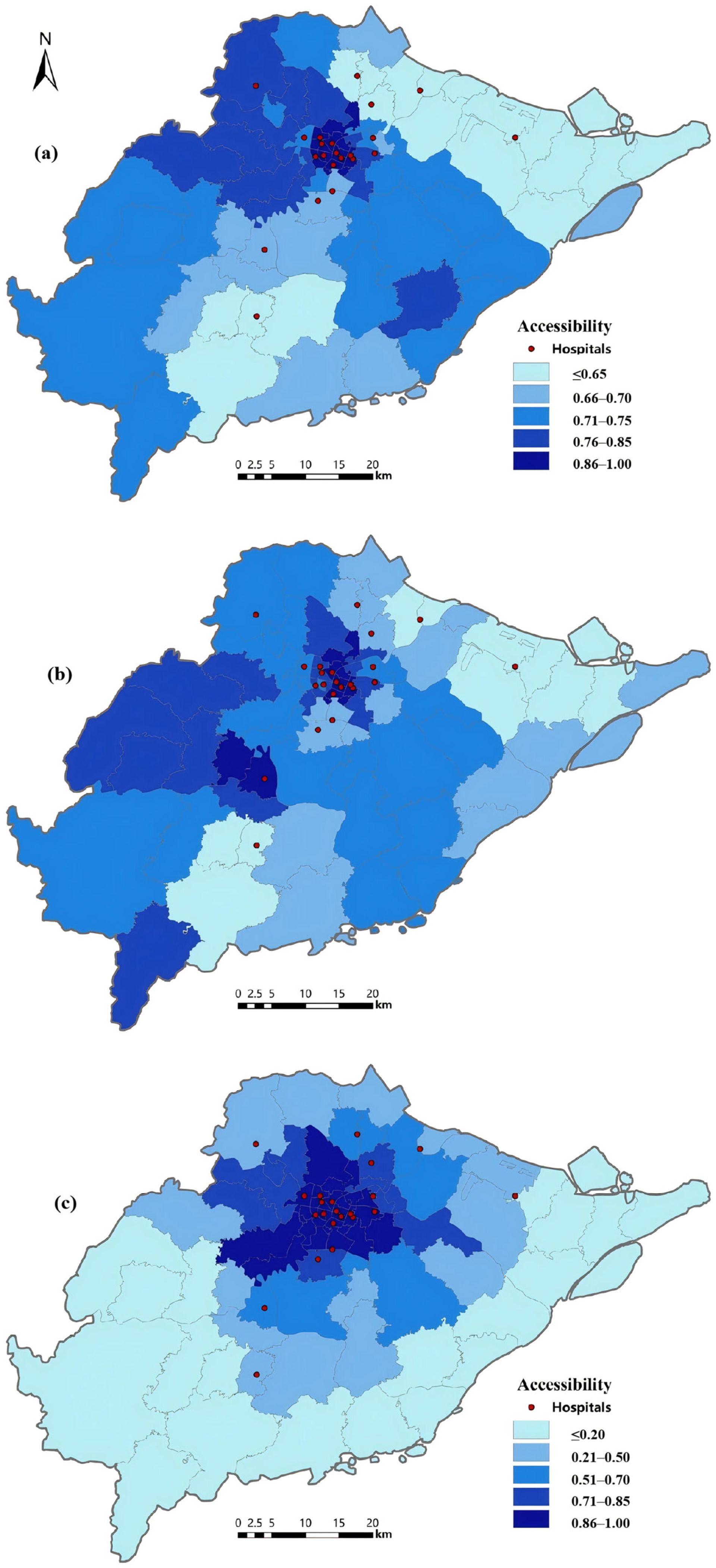
The BCEC-2SFCA model proposed in this study and the traditional Gaussian 2SFCA based on a fixed threshold exhibit systematic differences in characterizing the spatial pattern of accessibility to tertiary hospitals in Ningbo (Figure 8).

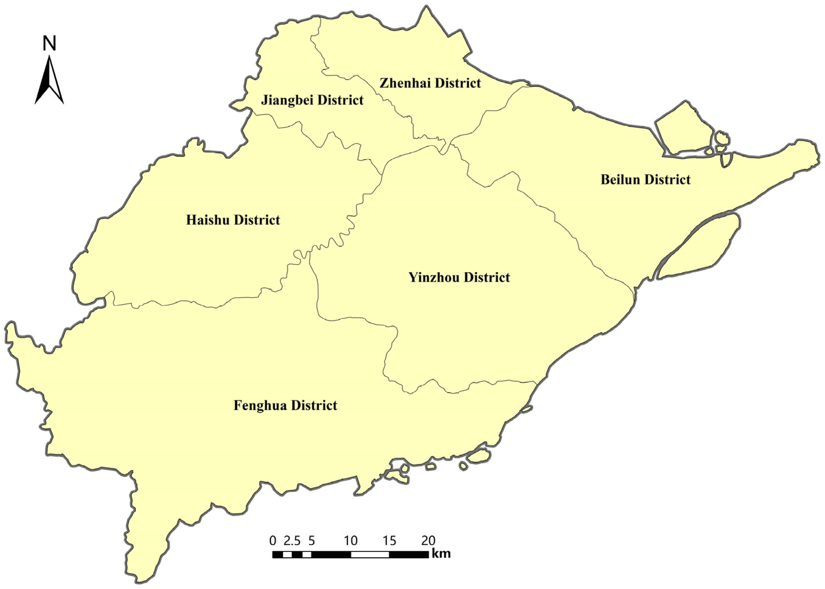
The results calculated by the BCEC-2SFCA model reveal significant spatial heterogeneity in the accessibility of tertiary hospitals in Ningbo. High-accessibility areas are highly concentrated in central urban districts such as Haishu, Jiangbei, and Yinzhou, forming accessibility peak zones centered around key hospitals like First Affiliated Hospital of Ningbo University (Yuehu and Waitan campuses) and Ningbo Medical Center Lihuili Hospital. This region has a high density of hospital resources, where residents’ choice sets overlap significantly, leading to pronounced competitive effects and consequently higher effective accessibility calculated by the model. Areas with lower accessibility are primarily distributed in Fenghua District and Beilun District.

A comparison between the BCEC-2SFCA model (travel time) and the BCEC-2SFCA model (travel distance) reveals that the accessibility distributions of the two models are generally similar, with the main differences located in the western part of Haishu District and the northern part of Fenghua District. To further assess the robustness of the proposed framework, we examined the consistency between accessibility estimates derived from travel time and travel distance. The two sets of accessibility scores exhibit a strong positive correlation, with a Pearson correlation coefficient of 0.845 (p < 0.001) and a Spearman rank correlation coefficient of 0.817 (p < 0.001). This strong agreement indicates that the behavioral core of the model—the Huff probability structure—is not unduly sensitive to the choice of impedance metric. Whether travel time or travel distance is used as the measure of spatial separation, the resulting accessibility patterns remain remarkably consistent, underscoring the stability and reliability of the BCEC-2SFCA approach.

Crucially, even in peripheral areas, the minimum standardized accessibility calculated by the BCEC-2SFCA model is 0.31, with no residential points being absolutely inaccessible (value of 0). This reflects the reality of residents’ healthcare-seeking behavior: even those in outer suburbs have a possibility (albeit low probability) of choosing to travel to major tertiary hospitals in the urban center.

In contrast, the spatial pattern presented by the Gaussian 2SFCA model with a fixed catchment size is markedly different. In this study, the fixed threshold of 45 min was selected for the Gaussian 2SFCA method. This choice was guided by two complementary considerations. First, based on the complete origin–destination travel time matrix, 98.15% of all observed hospital-oriented taxi trips fell within 45 min, confirming that this threshold captures the vast majority of actual healthcare-seeking travel behavior. Second, following a maximum–minimum distance principle, we computed for each of the 81 townships/subdistricts the travel time to its nearest tertiary hospital. The maximum of these nearest-hospital travel times across all townships was 40.29 min. Any threshold below this value would leave at least one township with no hospital within range. The adopted threshold of 45 min exceeds this lower bound, thereby ensuring complete spatial coverage of the study area while remaining firmly grounded in the observed travel time distribution. However, even with this adjustment, the disparities in the model results clearly reveal the systematic spatial bias inherent in traditional fixed-threshold models. The Gaussian 2SFCA model exhibits the following issues:

1.

Overestimation of accessibility in areas proximate and at intermediate distances to hospitals: Within close and intermediate proximity to tertiary hospitals, the Gaussian 2SFCA model overestimates accessibility. This is primarily attributed to the relatively slow decay of the Gaussian decay function over short distances. Furthermore, the longer the preset exogenous fixed threshold, the larger the zone of slow decay becomes, thereby amplifying this effect. Additionally, the Gaussian 2SFCA model fails to capture the “choice overload” and competitive effects resulting from the high concentration of hospitals in central urban areas. In the BCEC-2SFCA model, although residents in these areas face a multitude of high-quality hospitals, the choice weights derived from the Huff model concentrate their selections on a few nearest or most attractive hospitals. The influence of other neighboring hospitals is diluted due to competition, consequently lowering the comprehensive accessibility score. In contrast, the Gaussian model simply performs a linear summation of the influence of all hospitals within a 45 min range, overlooking the concentration of resident decision-making in contexts of abundant choice.

2.

Underestimation of accessibility in areas distant from hospitals: The Gaussian 2SFCA model significantly underestimates accessibility in regions farther from hospitals. This represents the primary bias identified in this study. On one hand, due to its fixed hard cutoff, the Gaussian model completely disregards the long-distance travel behavior of residents in peripheral areas seeking quality medical resources. Conversely, the BCEC-2SFCA model does not set a fixed threshold, this incorporates large core hospitals, which, despite being distant, still have a probability of being selected, into the effective choice set, thereby assigning more realistic accessibility values to these areas. On the other hand, the Gaussian decay function decays very rapidly over intermediate distances, resulting in extremely low weights for hospitals at long distances. Consequently, the Gaussian model produces a substantial accessibility disparity between central and peripheral areas.

5.2. Analysis of Accessibility Ranking Changes

To quantitatively assess the differences in evaluation results between the BCEC-2SFCA Model (Travel Time) and Gaussian 2SFCA Model, this section further compares the accessibility rankings of each region under both models. Changes in ranking directly reflect how the relative assessment of regional healthcare resource accessibility is systematically reconfigured when residents’ behavioral decisions are incorporated.

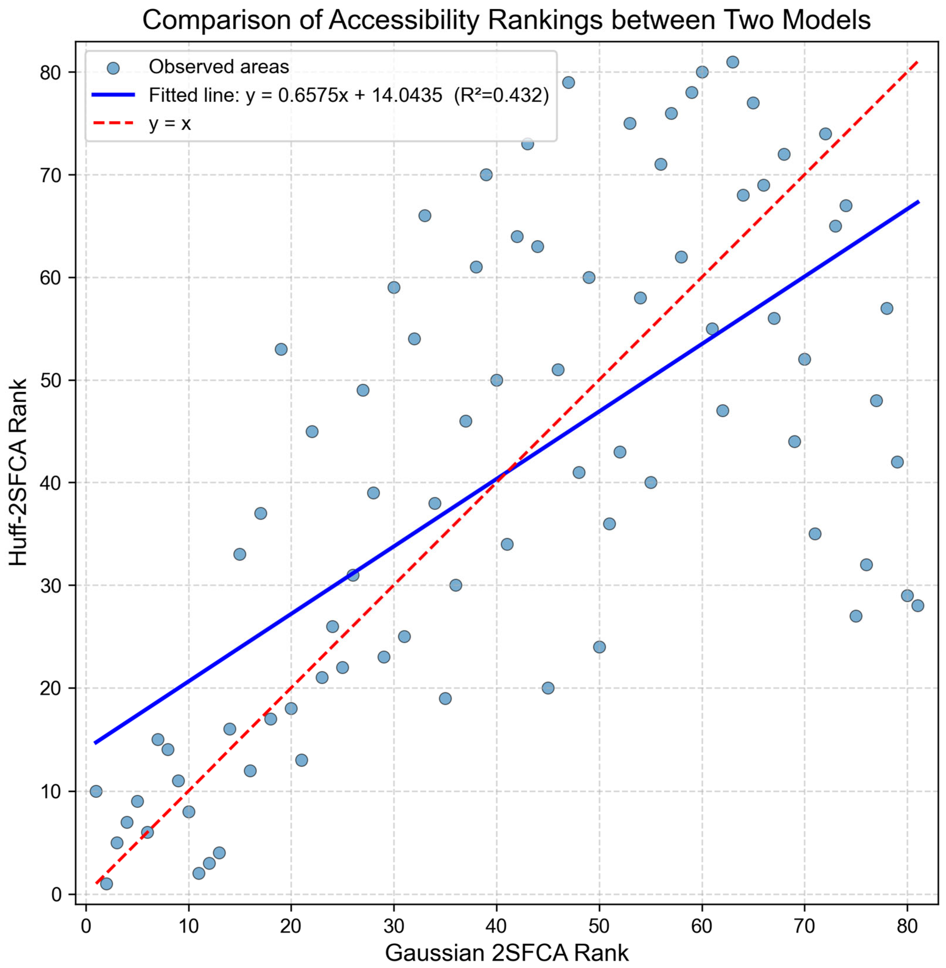
Among the 81 townships/subdistricts, the accessibility rankings derived from the two models exhibit a substantial reconfiguration. Overall, 37 areas (45.7%) experienced an increase in rank under the BCEC-2SFCA model compared to the Gaussian 2SFCA model, indicating that their relative level of healthcare resource accessibility was reassessed as higher after incorporating residents’ behavioral decisions. Conversely, 43 areas (53.1%) experienced a decrease in rank, with these areas predominantly concentrated in the hospital-dense central city and inner suburbs. Rankings for only 1 area (1.2%) remained unchanged, highlighting the widespread corrective effect of the behaviorally endogenous model on the assessment outcomes.

Figure 9 provides a visual comparison of the accessibility rankings for all townships/subdistricts under the two models using a scatter plot. Regarding the magnitude of change, the ranking shifts are more pronounced than those observed in preliminary analyses. The average increase for areas that rose in rank was 16.14 places, while the average decrease for areas that fell in rank was 13.88 places. These figures indicate that the BCEC-2SFCA model not only reorders many areas but also does so with considerable magnitude, particularly upgrading peripheral locations and downgrading some central ones.

To further quantify the linear relationship between the accessibility rankings derived from the two models, we performed an ordinary least squares regression using the Gaussian 2SFCA rankings as the independent variable (x) and the BCEC-2SFCA model rankings as the dependent variable (y). The fitted linear equation is:

$$y=0.6575\mathrm{x}+14.0435R^2=0.4323$$

(26)

The slope of 0.6575, being substantially less than 1, indicates a notable compression effect: the BCEC-2SFCA model tends to assign relatively lower rankings (i.e., worse positions) to many of the top-ranked areas under the Gaussian model, while assigning relatively higher rankings (i.e., better positions) to many of the lower-ranked areas. This aligns with the earlier observation that the BCEC-2SFCA model moderates extreme rankings, narrowing the accessibility gap between central and peripheral regions. The positive intercept of 14.0435 implies that, on average, the BCEC-2SFCA rankings are shifted upward (i.e., numerically larger, meaning less favorable) relative to the Gaussian rankings, especially for areas with very low Gaussian rankings (near the top). Conversely, for areas with very poor Gaussian rankings (large x values), the BCEC-2SFCA rankings become comparatively better than the linear trend would predict. The R² value of 0.4323 demonstrates a moderate linear association, confirming that the reconfiguration induced by the BCEC-2SFCA model is systematic, though with substantial scatter reflecting the model’s nuanced adjustments.

These regression results reinforce the conclusion that the BCEC-2SFCA model corrects the systematic biases of the fixed-threshold Gaussian model by moderating extreme rankings—downgrading overestimated central areas and upgrading underestimated peripheral regions—while still preserving a recognizable overall spatial order.

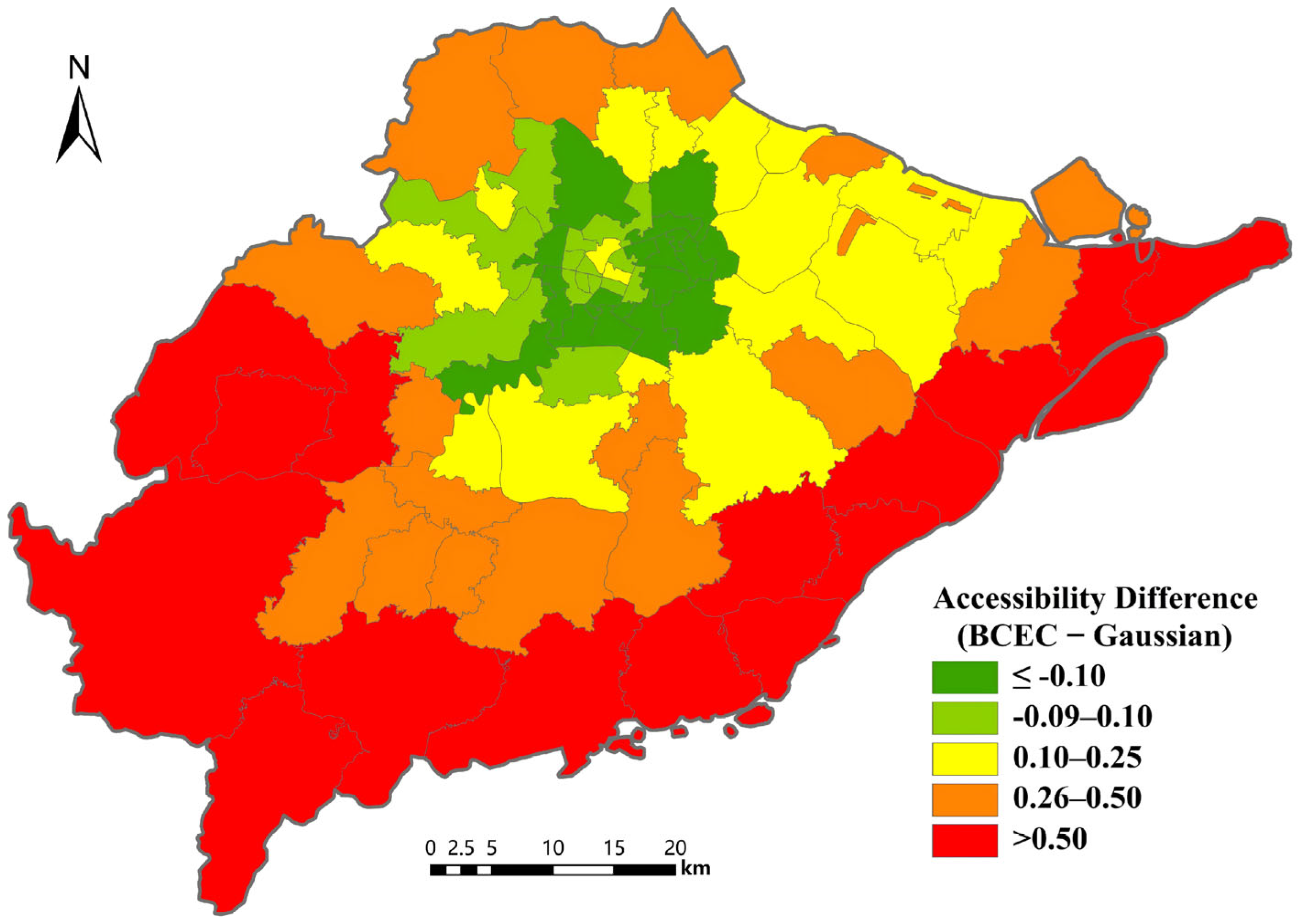
To further illustrate the spatial pattern of the adjustments introduced by the BCEC-2SFCA model, Figure 10 presents a difference map of the standardized accessibility scores, computed as BCEC-2SFCA minus Gaussian 2SFCA for each township/subdistrict. Green shades indicate negative differences (BCEC < Gaussian), representing areas where the BCEC-2SFCA model assigns lower accessibility than the Gaussian benchmark. These areas are predominantly concentrated in the central urban districts of Haishu, Jiangbei, and Yinzhou, reflecting the competition effect that moderates accessibility in hospital-dense locations. In contrast, yellow, orange, and red shades indicate positive differences (BCEC > Gaussian), representing areas where the BCEC-2SFCA model yields higher accessibility. These positive adjustments are most pronounced in the peripheral townships of Fenghua, Beilun, and Zhenhai districts, confirming that the endogenous search range mechanism substantially elevates accessibility estimates in outlying areas. The spatial divergence revealed by the difference map underscores the extent to which the BCEC-2SFCA framework corrects the systematic overestimation of central accessibility and underestimation of peripheral accessibility inherent in fixed-threshold Gaussian models.

5.3. Implications for Planning and Policy

The model differences lead directly to divergent assessments of whether regional medical resources are adequate, carrying clear policy implications.

1.

Re-evaluating “Service Blind Spots”: Although the Gaussian 2SFCA model did not generate “service blind spots” (areas with zero accessibility) in this study, its fixed threshold and hard cutoff still assume that residents in peripheral areas can only access services from a very limited number of hospitals. Consequently, the accessibility level in these areas remains extremely low. In contrast, under the BCEC-2SFCA model, the accessibility disparity between peripheral and central areas is significantly narrowed. For example, in certain townships or subdistricts of Fenghua District and Beilun District, the accessibility scores under the Gaussian model are extremely low, even approaching zero. However, under the BCEC model, they still maintain accessibility scores of approximately 0.3–0.4 and exhibit non-negligible choice probabilities for major hospitals in the city center. This finding implies that, for regions identified by traditional methods as severely resource-deficient, policy priorities should shift away from simply constructing new hospitals to fill absolute gaps (which may be economically inefficient and ineffective), towards strategies aimed at reducing the actual barriers residents face in accessing existing high-quality resources located farther away. For instance, establishing a direct express bus route connecting the western townships of Fenghua District to the Ningbo First Hospital area could substantially reduce travel time for residents in these peripheral communities, thereby improving effective accessibility without requiring new hospital construction. Similarly, expanding telemedicine services and streamlining referral pathways between community health centers in Beilun’s eastern townships and major tertiary hospitals could mitigate the burden of long-distance travel.

2.

Transformation in Resource Allocation Assessment: In the central districts of Haishu, Jiangbei, and Yinzhou, the BCEC-2SFCA model assigns lower accessibility scores than the Gaussian model for many townships, despite their proximity to multiple hospitals. This downward adjustment reflects the competition effect captured by the Huff choice probabilities: when many attractive hospitals are available, residents’ selections concentrate on a few preferred facilities, diluting the effective demand at neighboring hospitals. This finding implies that the marginal benefit of constructing new large hospitals in the urban core may be overestimated. Instead, resource investment should focus on systemic integration and functional differentiation—for instance, strengthening specialized departments at existing hospitals to reduce redundant competition and improve overall service efficiency.

3.

Methodological Implications: The systematic differences between the BCEC-2SFCA and Gaussian 2SFCA rankings—particularly the fact that the average rank adjustment for certain townships exceeds 10 positions—indicate that when assessing the accessibility of high-level, wide-coverage service facilities, the primary source of measurement error is not data precision, but erroneous a priori assumptions regarding residents’ behavioral search ranges. Adopting endogenous, behavior-based choice models to define the search range can fundamentally avoid the systematic spatial bias (overestimating the periphery, underestimating the center) caused by exogenous, rigid thresholds, providing a scientific basis for more equitable and effective spatial planning of healthcare.

In summary, the comparative analysis in this chapter demonstrates that, compared to the traditional Gaussian 2SFCA model, the BCEC-2SFCA framework generates a continuously varying and behaviorally plausible spatial picture of accessibility. It not only eliminates unrealistic “service blind spots” but also reveals competitive effects in resource-concentrated areas, providing a more reliable analytical foundation for precisely identifying shortcomings in the spatial allocation of medical resources and formulating differentiated improvement strategies.

6. Model Validation Using Hospital Outpatient Volume

To objectively evaluate the predictive capability of the proposed BCEC-2SFCA model in reproducing residents’ hospital choice distribution, this chapter employs annual hospital outpatient volume—a dataset independent of the model construction process—for validation. By comparing predicted shares with actual outpatient shares, we quantify the predictive accuracy of different models (the travel time-based BCEC-2SFCA model and the Gaussian 2SFCA method) and examine their stability across hospital types.

6.1. Data Preparation and Processing

6.1.1. Actual Outpatient Share $O_j$

Let Vj denote the annual outpatient volume of hospital j. The actual outpatient share $O_j$ of hospital j is defined as:

$$O_j={\displaystyle \frac{V_j}{{\displaystyle {\sum }_{m=1}^{N_h}} V_m}},j=\mathrm{1,2},\dots ,N_h$$

(27)

where $N_h=16$ is the total number of tertiary hospitals for which annual outpatient volume data were obtained.

6.1.2. Model-Predicted Outpatient Share ${\widehat{O}}_j^{\left(\mathrm{M}\right)}$

For any model M∈{BCEC-2SFCA, Ga2SFCA}, the predicted share ${\widehat{O}}_j^{\left(\mathrm{M}\right)}$ represents the proportion of total healthcare demand that the model allocates to hospital j.

1.

For the proposed model (BCEC-2SFCA), the predicted share is computed as:

$${\widehat{O}}_j^{\left(\mathrm{B}\mathrm{C}\mathrm{E}\mathrm{C}\right)}={\displaystyle \frac{{\displaystyle {\sum }_{i=1}^{N_d}} \left(D_i\times P_{ij}\right)}{{\displaystyle {\sum }_{i=1}^{N_d}} D_i}}$$

(28)

where:

$N_d=81$ is the number of demand points;

$D_i$ is the residential population of demand point i;

$P_{ij}$ the calibrated Huff choice probability;

2.

For the comparative model Ga2SFCA, its predicted share is calculated in accordance with its internal logic. Specifically, it is defined as the proportion of the weighted demand population visiting hospital j, as represented by the denominator in the first step of the model, relative to the total similarly weighted demand population citywide.

$${\widehat{O}}_j^{\left(\mathrm{G}\mathrm{a}\right)}={\displaystyle \frac{\sum _{i:t_{ij}\le d_0} D_i\cdot {G(t}_{ij},t_0)}{{\displaystyle {\sum }_{j=1}^{N_h}} \sum _{i:t_{ij}\le d_0} D_i\cdot {G(t}_{ij},t_0)}}$$

(29)

The numerator represents the Gaussian-weighted demand population that can reach hospital j, and the denominator is the total weighted demand attracted by all hospitals citywide.

6.2. Validation Metrics

To comprehensively compare the consistency between predicted and actual shares, the following metrics are adopted:

6.2.1. Correlation Metrics

Calculate two types of correlation coefficients between the predicted share series ${\widehat{O}}_j^{\left(M\right)}$ for each model and the actual share series $O_j$.

1.

Pearson Correlation Coefficient r: Measures the linear relationship between two series.

$$r^{\left(M\right)}={\displaystyle \frac{{\displaystyle {\sum }_{j=1}^{N_h}} \left(O_j-\overline{O}\right)\left({\widehat{O}}_j^{\left(M\right)}-{\overline{\widehat{O}}}^{\left(M\right)}\right)}{\sqrt{{\displaystyle {\sum }_{j=1}^{N_h}} (O_j-\overline{O}{)}^2\cdot {\displaystyle {\sum }_{j=1}^{N_h}} ({\widehat{O}}_j^{\left(M\right)}-{\overline{\widehat{O}}}^{\left(M\right)}{)}^2}}}$$

(30)

where $\overline{O}$ and ${\overline{\widehat{O}}}^{\left(M\right)}$ denote the means of the respective series.

2.

Spearman Rank Correlation Coefficient ρ: Assesses the monotonic relationship, robust to outliers.

$${\rho }^{\left(M\right)}=1-{\displaystyle \frac{6{\displaystyle {\sum }_{j=1}^{N_h}} (R_j^O-R_j^{\widehat{O}}{)}^2}{N_h\left(N_h^2-1\right)}}$$

(31)

where $R_j^O$ and $R_j^{\widehat{O}}$ are the ranks of $O_j$ and ${\widehat{O}}_j^{\left(M\right)}$, respectively.

6.2.2. Error Metrics

Calculate the prediction errors of each model.

1.

Root Mean Square Error (RMSE): Reflects the average magnitude of prediction errors.

$${\mathrm{R}\mathrm{M}\mathrm{S}\mathrm{E}}^{\left(M\right)}=\sqrt{{\displaystyle \frac{1}{N_h}}{\displaystyle \sum _{j=1}^{N_h}} {\left(O_j-{\widehat{O}}_j^{\left(M\right)}\right)}^2}$$

(32)

2.

Mean Absolute Percentage Error (MAPE): Expresses relative error in percentage terms.

$${\mathrm{M}\mathrm{A}\mathrm{P}\mathrm{E}}^{\left(M\right)}={\displaystyle \frac{100\%}{N_h}}{\displaystyle \sum _{j=1}^{N_h}} \left|{\displaystyle \frac{O_j-{\widehat{O}}_j^{\left(M\right)}}{O_j}}\right|$$

(33)

6.3. Validation Results

This section validates the predictive accuracy of the BCEC-2SFCA model against the Gaussian 2SFCA model using annual outpatient volume data from 16 tertiary hospitals in Ningbo for which such data are available. The actual outpatient share $O_j$ is computed by Equation (27); the predicted shares ${\widehat{O}}_j^{\left(BCEC\right)}$ and ${\widehat{O}}_j^{\left(Ga\right)}$ are obtained from Equation (28) and Equation (29), respectively. Four metrics are employed: Pearson correlation coefficient, Spearman rank correlation coefficient, root mean square error (RMSE), and mean absolute percentage error (MAPE).

Table 5. Comparison of validation metrics (based on 16 hospitals).

Metric	BCEC-2SFCA Model	Gaussian 2SFCA Model
Pearson’s r	0.5682 (p = 0.0216)	0.1163 (p = 0.6679)
Spearman’s ρ	0.5265 (p = 0.0362)	0.0529 (p = 0.8456)
RMSE	0.02700	0.02211
MAPE	32.17%	42.12%

summarizes the validation results. The BCEC-2SFCA model achieves a Pearson correlation of 0.5682 (p = 0.0216) and a Spearman rank correlation of 0.5265 (p = 0.0362), indicating a moderately strong and statistically significant monotonic relationship with the actual outpatient shares. In contrast, the Gaussian 2SFCA model yields much weaker correlations: Pearson 0.1163 (p = 0.6679) and Spearman 0.0529 (p = 0.8456). This demonstrates that the BCEC-2SFCA model is considerably more capable of replicating the relative order of hospital attractiveness and the competitive effects captured by real-world choice behavior.

Regarding prediction errors, the BCEC-2SFCA model yields a lower MAPE (32.17% vs. 42.12%), suggesting that its empirically calibrated choice probabilities better capture the relative distribution of patient demand across hospitals. However, its RMSE (0.02700) is slightly higher than that of the Gaussian 2SFCA model (0.02211), indicating that while the BCEC-2SFCA model excels at replicating the rank order of hospital attractiveness, it does not uniformly achieve lower absolute errors across all facilities. This trade-off underscores that the model’s primary strength lies in capturing competitive effects and relative attractiveness rather than minimizing aggregate absolute prediction error.

Overall, the validation results confirm that the proposed BCEC-2SFCA framework, with its empirically calibrated parameters and behaviorally derived choice probabilities, provides a more plausible representation of residents’ hospital-seeking behavior in terms of ranking and spatial competition than the conventional fixed-threshold Gaussian 2SFCA model. However, this improved behavioral realism does not translate into uniformly superior absolute predictive accuracy. The framework is therefore particularly suited for evaluating the relative accessibility of high-order medical services, where capturing competition and patient choice is more critical than minimizing absolute prediction error.

To further examine whether model performance varies by hospital type, a supplementary subgroup analysis was conducted. The 16 hospitals with available outpatient data were divided into two groups based on the median number of beds: larger hospitals (≥1014 beds, N = 8) and smaller hospitals (<1014 beds, N = 8). For the larger hospitals, the BCEC-2SFCA model achieved a Pearson correlation of 0.192 and a Spearman rank correlation of 0.262, compared with 0.007 and −0.214 for the Gaussian model. The RMSE and MAPE for BCEC-2SFCA were 0.0219 and 23.9%, respectively, versus 0.0311 and 34.9% for the Gaussian model. For the smaller hospitals, BCEC-2SFCA yielded a Pearson correlation of 0.458 and a Spearman rank correlation of 0.548, whereas the Gaussian model produced values of −0.103 and 0.024. In this subgroup, BCEC-2SFCA had a lower MAPE (31.9% vs. 34.5%) but a slightly higher RMSE (0.0270 vs. 0.0242).

Although the reduced sample size in each subgroup precludes definitive statistical inference (none of the correlations reached conventional significance levels), the pattern of results is consistent with the full-sample findings: the BCEC-2SFCA model consistently outperforms the Gaussian benchmark in capturing the relative attractiveness of hospitals, regardless of hospital scale. The absolute prediction errors remain modest for larger hospitals but increase for smaller ones—a challenge common to both models and likely attributable to the greater volatility and lower absolute volumes of outpatient visits at smaller facilities. This exploratory analysis suggests that the BCEC-2SFCA framework maintains its behavioral advantage across heterogeneous hospital types, while also highlighting the inherent difficulty of predicting demand for smaller, lower-volume hospitals. Future work with larger validation samples could more rigorously assess the boundary conditions of the proposed approach.

6.4. Robustness Check: Model Calibration with All 22 Tertiary Hospitals

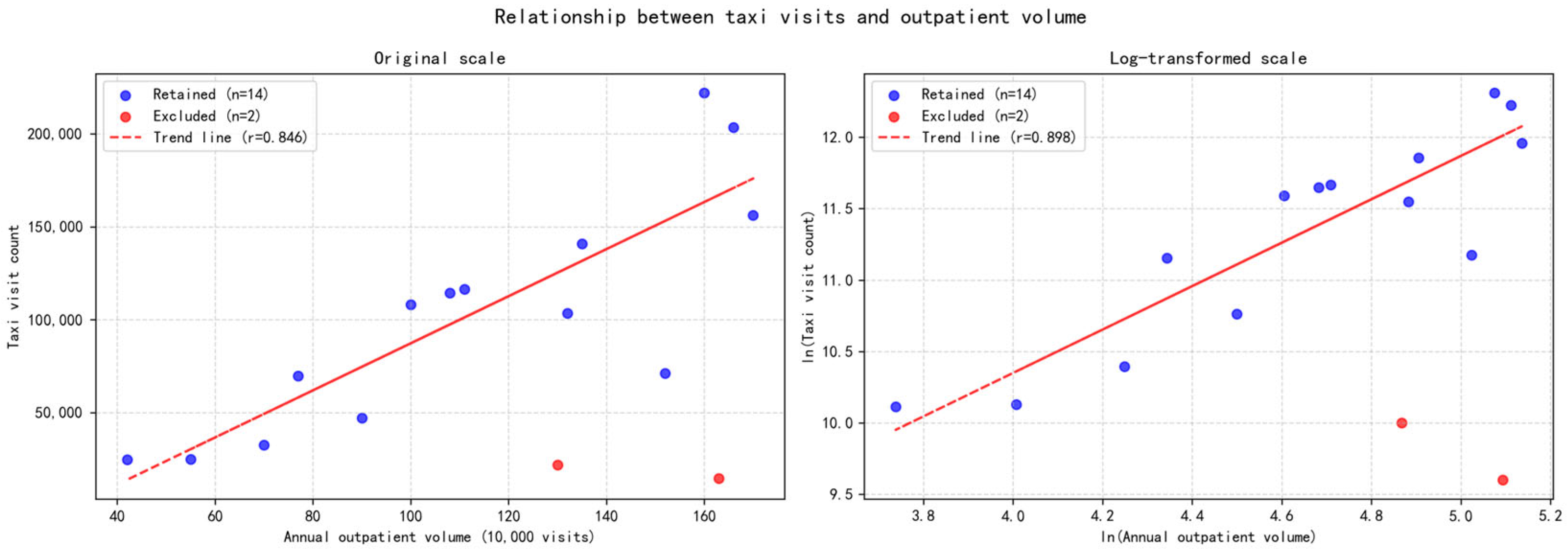
To assess the sensitivity of the parameter estimates to the composition of the calibration sample, we repeated the log-centered OLS calibration using all 22 tertiary hospitals located within the study area (1782 OD pairs; 81 townships × 22 hospitals). The estimated parameters were $\alpha$ = 0.9586 (p < 0.001) and $\beta$ = 3.0685 (p < 0.001), with $R^2$ = 0.620. These values are comparable in magnitude and statistical significance to the estimates obtained from the 14-hospital subset used in the main analysis ($\alpha$ = 1.1758, $\beta$ = 2.9608, $R^2$ = 0.665).

Using the alternatively calibrated parameters, we recomputed the BCEC-2SFCA accessibility scores and the predicted outpatient shares for the 16 hospitals with available outpatient data. The resulting validation metrics are as follows: Pearson’s r = 0.505 (p = 0.046), Spearman’s ρ = 0.541 (p = 0.030), RMSE = 0.0254, and MAPE = 28.20%. For comparison, the 14-hospital calibration yielded Pearson’s r = 0.568, Spearman’s ρ = 0.527, RMSE = 0.027, and MAPE = 32.17%. The performance of the BCEC-2SFCA model under the 22-hospital calibration remains very close to that of the main calibration, and both substantially outperform the Gaussian 2SFCA benchmark (Pearson’s r = 0.116, Spearman’s ρ = 0.053, RMSE = 0.022, MAPE = 42.12%).

The slight variations in parameter estimates and validation metrics are expected, as the 14-hospital subset was selected to maximize the reliability of the taxi-based proxy. Nevertheless, the consistency of the results across the two calibration samples confirms that the core findings of this study are not sensitive to the specific composition of the calibration sample.

7. Discussion

The validation results presented in this study highlight a trade-off: the BCEC-2SFCA model excels at capturing the rank order of hospital attractiveness ($Spearman’s \rho =0.527$) and relative demand distribution (MAPE = 32.17%), but its RMSE (0.02700) is slightly higher than that of the Gaussian model (0.02211). This indicates that the model’s primary strength lies in replicating competitive dynamics rather than minimizing absolute prediction error.

The strong correlation between travel-time and travel-distance accessibility ($Pearson r=0.845, Spearman’s \rho =0.817$) further supports the robustness of the approach, suggesting that the model’s behavioral core is stable across different impedance specifications. This consistency enhances confidence in its applicability to diverse data contexts.

The findings of this study can be situated within the broader literature on Huff-based FCA methods. Compared to Jin and Lu [30], who applied a multi-mode Huff-2SFCA to food accessibility, the present study extends the Huff-FCA framework to the healthcare domain while additionally calibrating the Huff parameters from observed travel behavior rather than relying on sensitivity tests. Relative to Subal et al. [31], who incorporated a Gaussian distance-decay function into a Huff-3SFCA model, our approach eliminates the need for predefined decay parameters entirely by letting the probability surface emerge from empirical data. The generalized flow-based 2SFCA of Chen et al. [34] shares with our work the use of taxi trajectory data; however, their method still relies on adaptive catchment delineation, whereas BCEC-2SFCA generates endogenous search ranges probabilistically without any spatial cutoff. These comparisons highlight that the key advancement of BCEC-2SFCA lies not in any single component but in the systematic integration of empirical calibration, real-world impedance, and endogenous catchment generation into a unified accessibility framework.

From a theoretical standpoint, this study contributes to the accessibility literature by demonstrating that the conventional dichotomy between “accessible” and “inaccessible”—embedded in all threshold-based 2SFCA variants—can be replaced with a continuous, competition-sensitive probability gradient. This shift from binary to probabilistic accessibility aligns the methodological framework more closely with the continuous nature of spatial behavior described in classical geography and with discrete choice theory in transportation research. Furthermore, the empirical calibration of Huff parameters from passive mobility data suggests a pathway toward behaviorally grounded accessibility models that reduce reliance on stated-preference surveys or ad hoc parameter assumptions, thereby enhancing the replicability and context-specificity of accessibility assessments.

Nevertheless, several limitations warrant acknowledgment. First, the use of taxi trajectory data does not capture all modes of healthcare travel; future work should integrate multi-source mobility data such as public transit smart card records or mobile phone signaling. Second, hospital attractiveness is represented solely by bed count, ignoring specialty mix, reputation, or insurance acceptance. Incorporating such attributes could refine the choice probabilities. Third, due to the unavailability of patient origin–destination flow data from hospital records—a common constraint in healthcare accessibility research—direct validation against actual patient flow patterns at the subdistrict level was not feasible. Nevertheless, the taxi trajectory data used for model calibration provide a large-scale proxy of revealed healthcare travel behavior, and the outpatient volume data offer an independent, facility-level benchmark for external validation. Fourth, the relatively small number of hospitals with available outpatient data (N = 16) precluded meaningful subsample analyses by region or hospital scale. Such analyses would require a substantially larger sample to retain statistical power within each subgroup. Future work could revisit these validation dimensions should more granular patient flow data or expanded outpatient datasets become available.

From a policy perspective, the findings suggest that resource allocation strategies should account for the competitive dynamics revealed by the BCEC-2SFCA model. In central urban areas, where accessibility is already high, further expansion of hospital capacity may yield diminishing returns due to competition; instead, efforts could focus on service integration and differentiation. In peripheral areas, improving transport connections to existing high-quality hospitals may be more effective than building new facilities, as residents already demonstrate a willingness to travel longer distances when necessary.

8. Conclusions

This study proposed a data-driven BCEC-2SFCA framework for assessing spatial accessibility to tertiary hospitals, using taxi trajectory data to empirically calibrate the Huff model parameters and to construct realistic travel impedance matrices. The framework was applied to Ningbo, China, with data from 22 tertiary hospitals, 81 townships/subdistricts, and over 1.58 million taxi trips. The main findings are as follows:

Empirically grounded parameters: The calibrated service capacity elasticity ($\alpha =1.1758$) and time decay coefficient ($\beta =2.9608$) reflect residents’ strong preference for larger hospitals and high sensitivity to travel time, providing a behaviorally realistic foundation for accessibility modeling.

Competition effects and spatial equity: The BCEC-2SFCA model captures competition among hospitals, moderating accessibility estimates in hospital-dense central areas while avoiding the underestimation of accessibility in peripheral regions that plagues fixed-threshold models. This yields a continuously varying and equitable spatial distribution.

Robustness to impedance metrics: Accessibility results based on travel time and travel distance are highly correlated ($Pearson r=0.845, Spearman’s \rho =0.817$), indicating that the model’s core mechanism is stable across different measures of spatial separation.

Predictive performance: Validation against annual outpatient volumes shows that the BCEC-2SFCA model excels at capturing the relative order of hospital attractiveness (Spearman ρ = 0.527) and relative demand distribution (MAPE = 32.17%), though its RMSE (0.02700) is slightly higher than that of the Gaussian model (0.02211). This trade-off underscores the model’s strength in replicating competitive dynamics rather than minimizing absolute prediction error.

Policy implications: The model highlights the need for differentiated strategies: in central areas, optimizing existing resources rather than expanding capacity; in peripheral areas, improving transport connectivity to overcome spatial barriers. The use of passive mobility data offers a scalable approach to dynamically monitor healthcare-seeking behavior.

In conclusion, the BCEC-2SFCA framework integrates empirically calibrated behavioral parameters and real-world travel data to produce more realistic and policy-relevant accessibility assessments. It should be reiterated that this framework is tailored specifically to high-order medical services such as tertiary hospitals, where facility competition and patient choice are central to travel behavior. For primary care or other services characterized by localized catchments, traditional threshold-based models may be more appropriate.

Future work could proceed in several directions. First, integrating additional mobility data sources—such as public transit smart card records, mobile phone signaling, and ambulance dispatch logs—would enable the calibration of mode-specific impedance matrices and better capture the healthcare travel behavior of underrepresented groups, including the elderly and low-income populations. Second, hospital attractiveness could be represented through a multi-dimensional index incorporating specialty mix, physician expertise, patient satisfaction, and insurance acceptance, rather than bed count alone. Third, the temporal dynamics of healthcare accessibility could be explored by extending the BCEC-2SFCA framework to account for diurnal and seasonal variations in traffic conditions and hospital service availability. Fourth, the generalizability of the framework should be tested in other urban contexts with different spatial configurations of healthcare resources, as well as for other types of high-order public services such as regional cultural centers and specialized elderly care facilities. Finally, coupling the BCEC-2SFCA model with spatial optimization algorithms could provide decision-support tools for equitable and efficient healthcare resource allocation.