Figure 1.
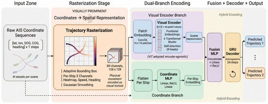
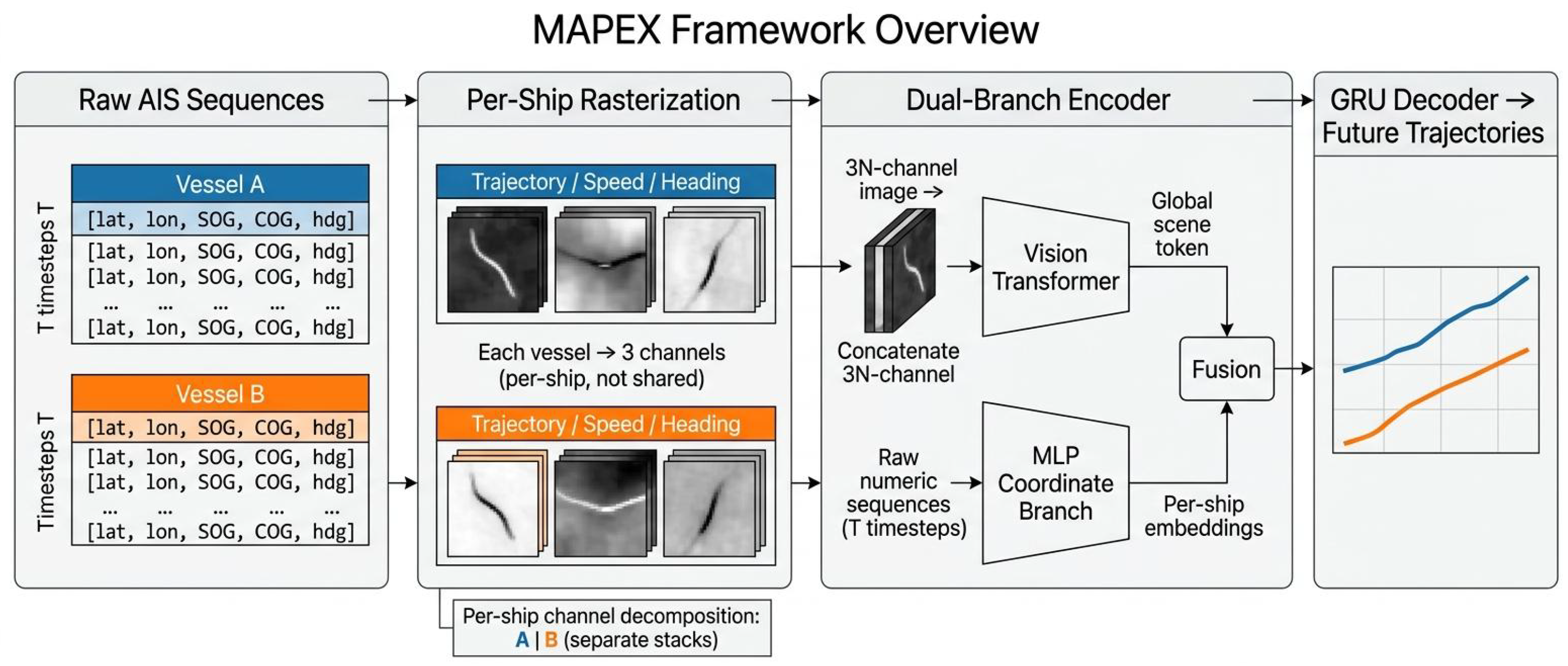
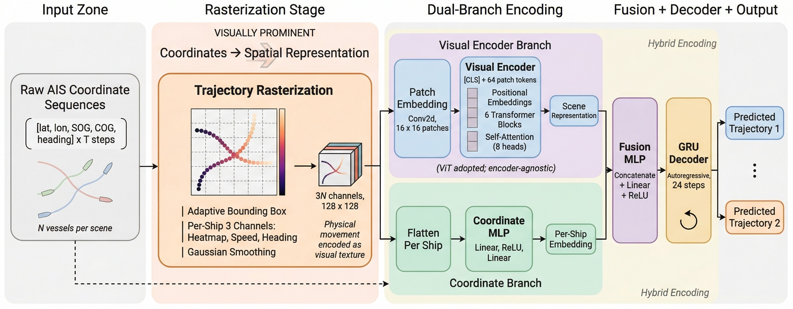
Overview of the Mapex framework. Raw AIS coordinate sequences for all vessels are co-registered onto a single shared canvas defined by one common adaptive bounding box, and each vessel contributes its own three channels (trajectory heatmap, speed field, heading field) on that shared canvas, yielding a -channel scene tensor; the per-vessel decomposition is along the channel axis, so the multiple trajectories visible in the localization panel correspond to per-vessel channels rendered on the same coordinate frame rather than to a single mixed-channel image. A visual encoder extracts a global scene representation, which is fused with per-ship coordinate embeddings from a parallel numeric branch. The fused representation feeds an autoregressive GRU decoder that predicts future trajectories for all vessels. Per-vessel channels are rendered with vessel-specific hues.
Figure 1.
Overview of the Mapex framework. Raw AIS coordinate sequences for all vessels are co-registered onto a single shared canvas defined by one common adaptive bounding box, and each vessel contributes its own three channels (trajectory heatmap, speed field, heading field) on that shared canvas, yielding a -channel scene tensor; the per-vessel decomposition is along the channel axis, so the multiple trajectories visible in the localization panel correspond to per-vessel channels rendered on the same coordinate frame rather than to a single mixed-channel image. A visual encoder extracts a global scene representation, which is fused with per-ship coordinate embeddings from a parallel numeric branch. The fused representation feeds an autoregressive GRU decoder that predicts future trajectories for all vessels. Per-vessel channels are rendered with vessel-specific hues.
Figure 2.
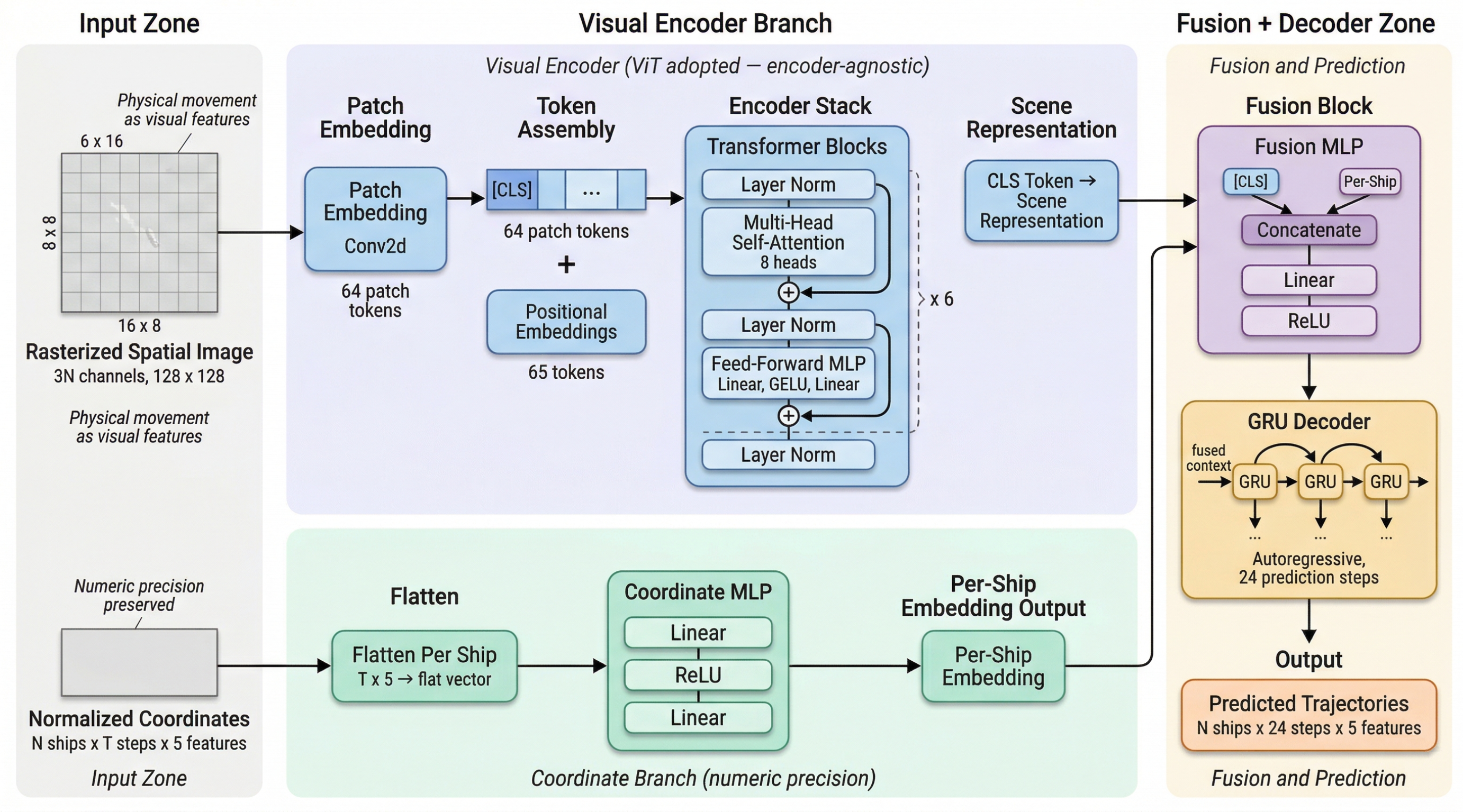
Detailed architecture of Mapex. Left: the rasterization pipeline converts N vessels’ coordinate sequences into a -channel spatial image. Center: a visual encoder (ViT with 6 blocks, 8 heads, ) processes 64 patches from the image, producing a CLS token as global scene representation. A parallel coordinate branch (MLP, ) preserves per-ship numeric precision. Right: the fusion MLP combines both streams, and an autoregressive GRU decoder generates 24-step predictions for each vessel.
Figure 2.
Detailed architecture of Mapex. Left: the rasterization pipeline converts N vessels’ coordinate sequences into a -channel spatial image. Center: a visual encoder (ViT with 6 blocks, 8 heads, ) processes 64 patches from the image, producing a CLS token as global scene representation. A parallel coordinate branch (MLP, ) preserves per-ship numeric precision. Right: the fusion MLP combines both streams, and an autoregressive GRU decoder generates 24-step predictions for each vessel.
Figure 3.
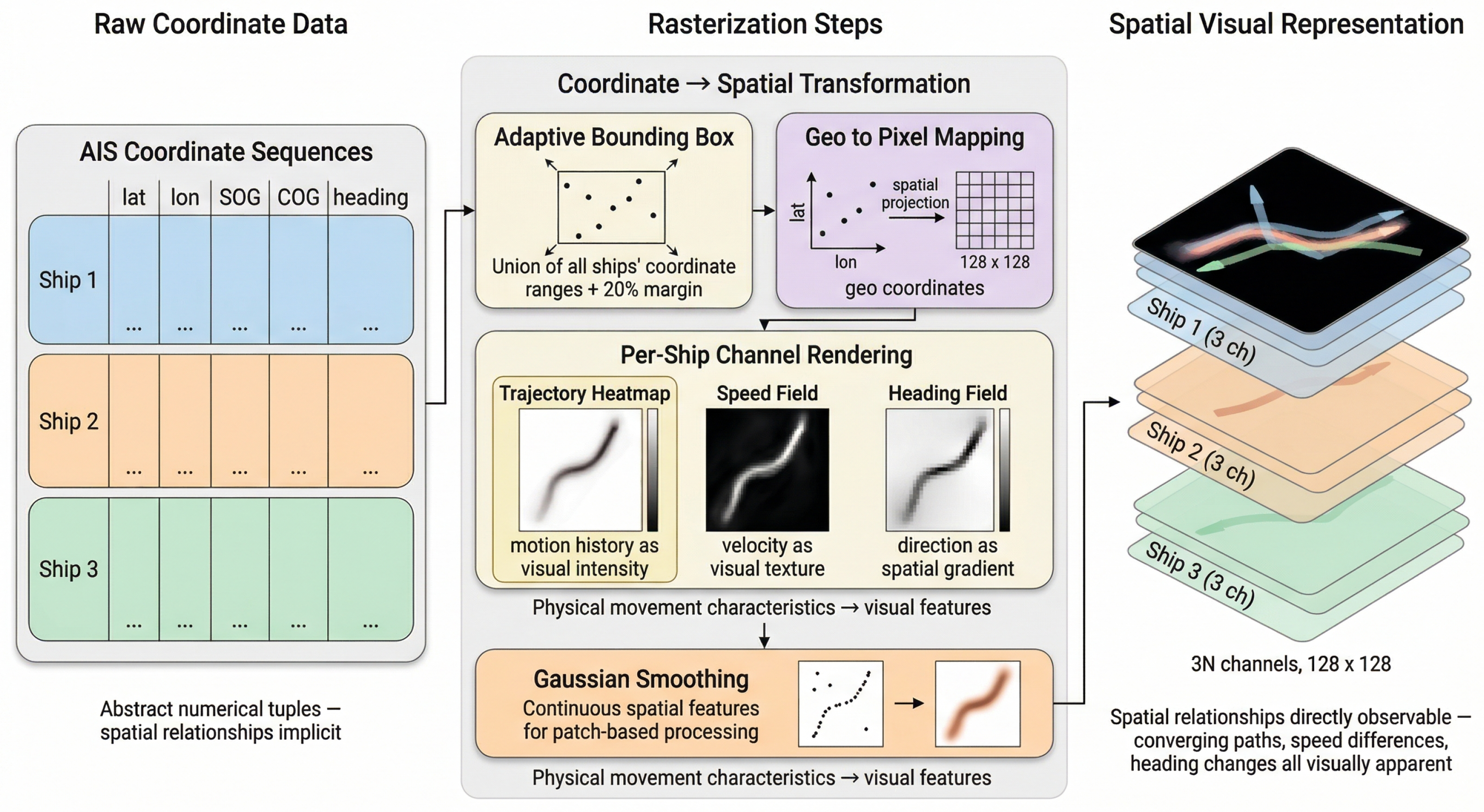
Trajectory rasterization pipeline. Raw AIS coordinates for multiple vessels are mapped to a canvas with an adaptive bounding box (20% margin). Each vessel produces three channels: trajectory heatmap with temporal gradient (brighter = more recent), speed field, and heading field. The resulting multi-channel image captures the complete observable state of the multi-vessel encounter as a spatial visual representation.
Figure 3.
Trajectory rasterization pipeline. Raw AIS coordinates for multiple vessels are mapped to a canvas with an adaptive bounding box (20% margin). Each vessel produces three channels: trajectory heatmap with temporal gradient (brighter = more recent), speed field, and heading field. The resulting multi-channel image captures the complete observable state of the multi-vessel encounter as a spatial visual representation.
Figure 4.
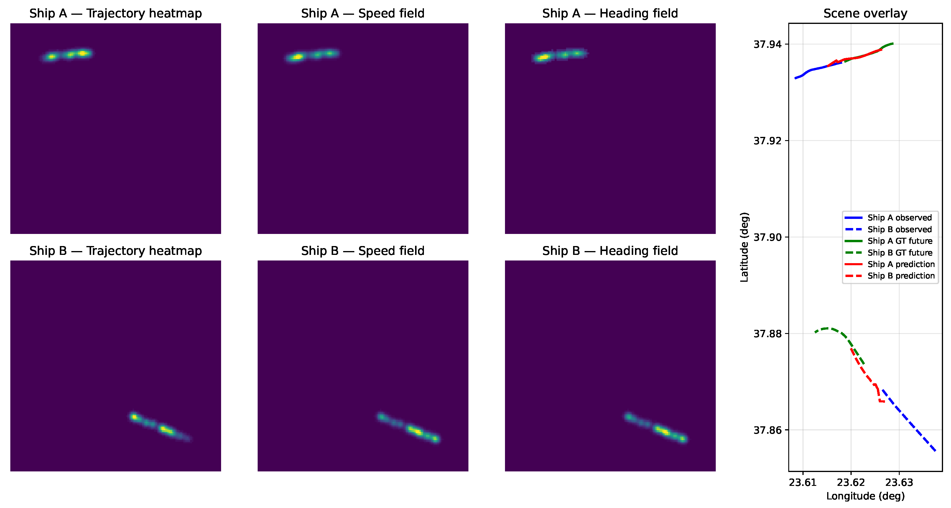
End-to-end Mapex on a representative pairwise encounter from the Piraeus test set. Six left panels: actual rendered input channels for both vessels (Ship A row, Ship B row); columns show the trajectory heatmap (temporal gradient: brighter = more recent), the speed field, and the heading field. Right panel: scene overlay with observed history (blue), ground-truth future (green), and Mapex prediction (red) on the adaptive bounding-box coordinate frame. The heatmap panels are rendered on the fixed square canvas that the model actually consumes; because the adaptive bounding box is generally non-square in degrees, the apparent slope of a track on the canvas differs from its geographic slope in the scene overlay by the bounding-box aspect ratio. The chosen sample contains a non-trivial maneuver to make the model behavior visible, so the individual ADE is naturally above the dataset-wide 5-seed mean of nm.
Figure 4.
End-to-end Mapex on a representative pairwise encounter from the Piraeus test set. Six left panels: actual rendered input channels for both vessels (Ship A row, Ship B row); columns show the trajectory heatmap (temporal gradient: brighter = more recent), the speed field, and the heading field. Right panel: scene overlay with observed history (blue), ground-truth future (green), and Mapex prediction (red) on the adaptive bounding-box coordinate frame. The heatmap panels are rendered on the fixed square canvas that the model actually consumes; because the adaptive bounding box is generally non-square in degrees, the apparent slope of a track on the canvas differs from its geographic slope in the scene overlay by the bounding-box aspect ratio. The chosen sample contains a non-trivial maneuver to make the model behavior visible, so the individual ADE is naturally above the dataset-wide 5-seed mean of nm.
Figure 5.
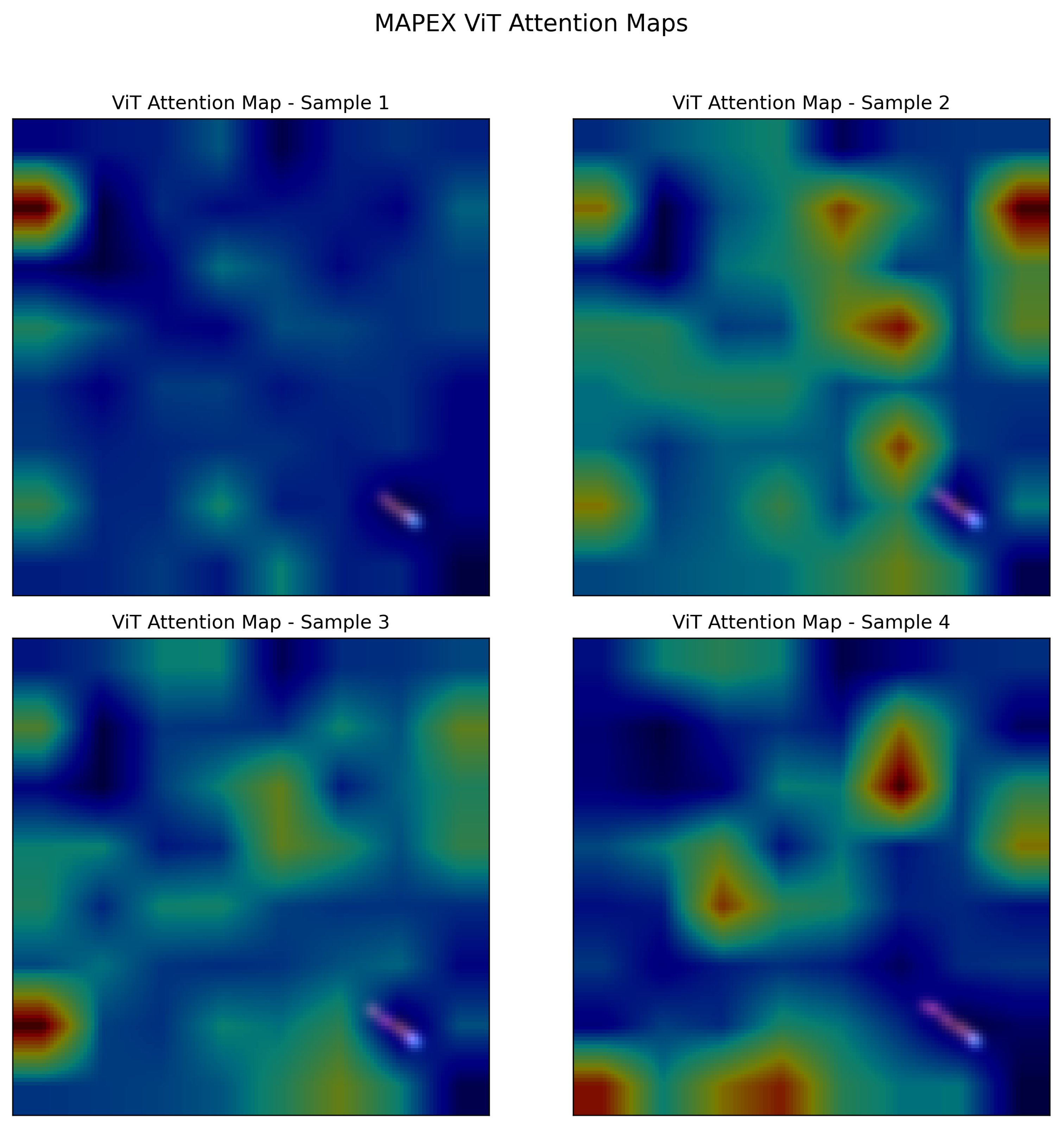
CLS token attention maps from the final ViT Transformer block across four encounter samples. Warmer colors indicate higher attention weights. The model consistently attends to trajectory intersection regions and vessel endpoints.
Figure 5.
CLS token attention maps from the final ViT Transformer block across four encounter samples. Warmer colors indicate higher attention weights. The model consistently attends to trajectory intersection regions and vessel endpoints.
Figure 6.
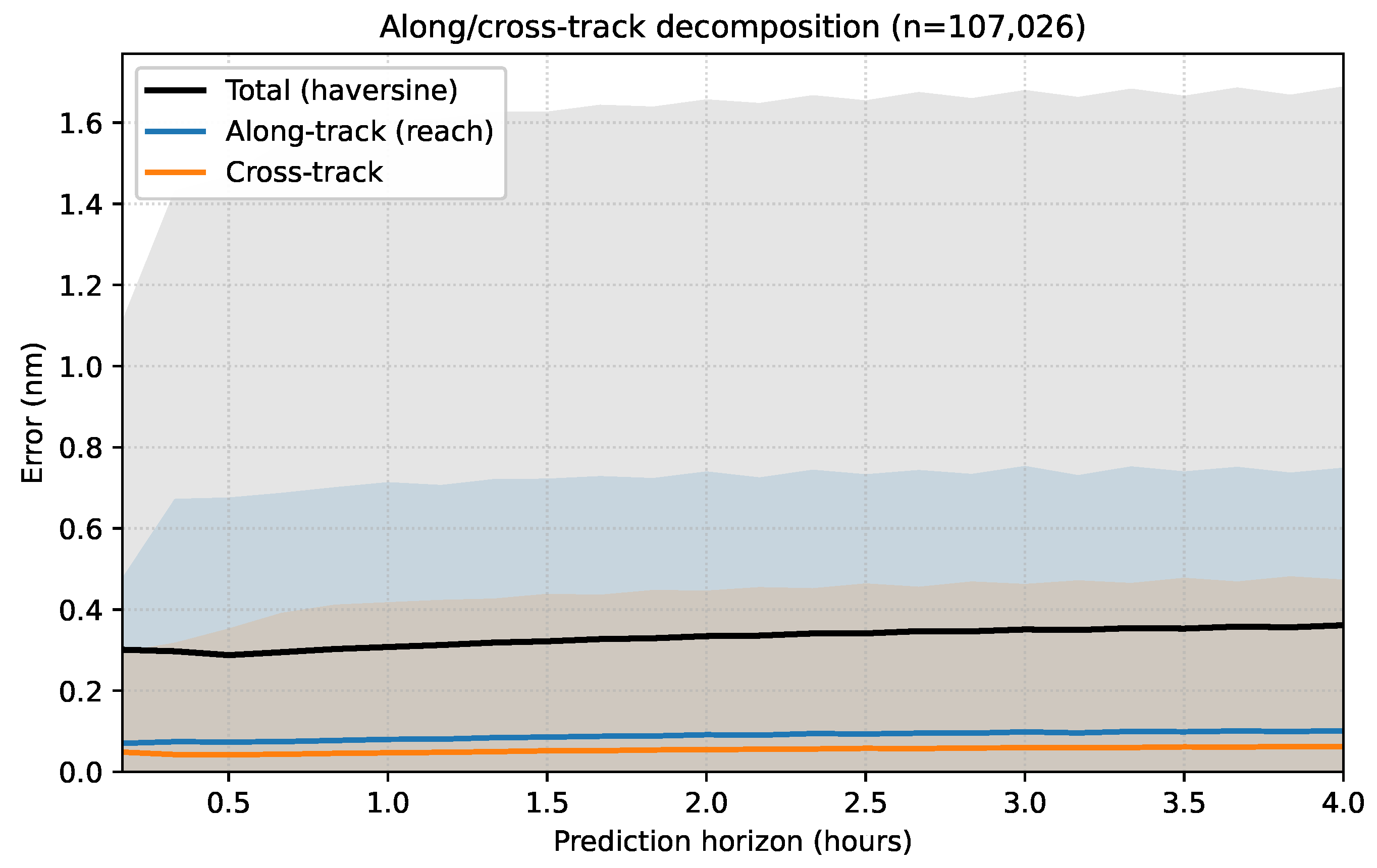
Per-step prediction error over the 24-step horizon (4 h at 10-min intervals) decomposed into along-track (reach, parallel to ground-truth velocity) and cross-track (perpendicular) components, with std bands. Evaluated on the v2 MMSI-strict test split ( predicted trajectories, seed 42). The total haversine error grows gradually rather than exponentially, and the decomposition shows that along-track error dominates throughout the horizon, with cross-track error staying small and nearly flat.
Figure 6.
Per-step prediction error over the 24-step horizon (4 h at 10-min intervals) decomposed into along-track (reach, parallel to ground-truth velocity) and cross-track (perpendicular) components, with std bands. Evaluated on the v2 MMSI-strict test split ( predicted trajectories, seed 42). The total haversine error grows gradually rather than exponentially, and the decomposition shows that along-track error dominates throughout the horizon, with cross-track error staying small and nearly flat.
Figure 7.
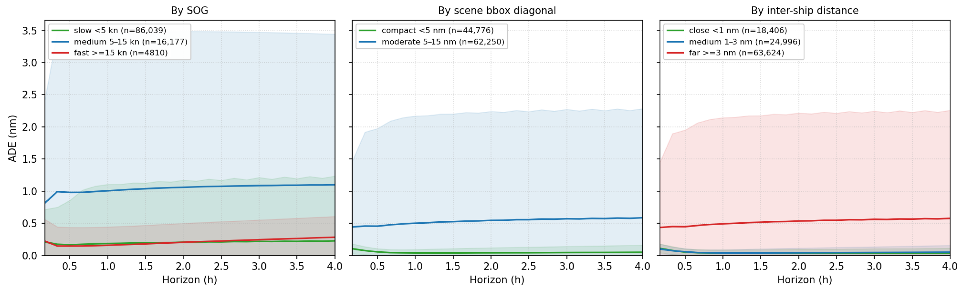
Per-step ADE over the 4-h horizon stratified by (left) speed over ground, (middle) scene bbox diagonal, and (right) inter-ship distance, with std bands. Bins with zero samples (e.g., wide scenes nm in the Piraeus test split) are omitted. Close-passage pairs (<1 nm, ) are not systematically harder than medium-distance pairs, confirming that the shared-canvas representation does not blur close from far encounters.
Figure 7.
Per-step ADE over the 4-h horizon stratified by (left) speed over ground, (middle) scene bbox diagonal, and (right) inter-ship distance, with std bands. Bins with zero samples (e.g., wide scenes nm in the Piraeus test split) are omitted. Close-passage pairs (<1 nm, ) are not systematically harder than medium-distance pairs, confirming that the shared-canvas representation does not blur close from far encounters.
Figure 8.
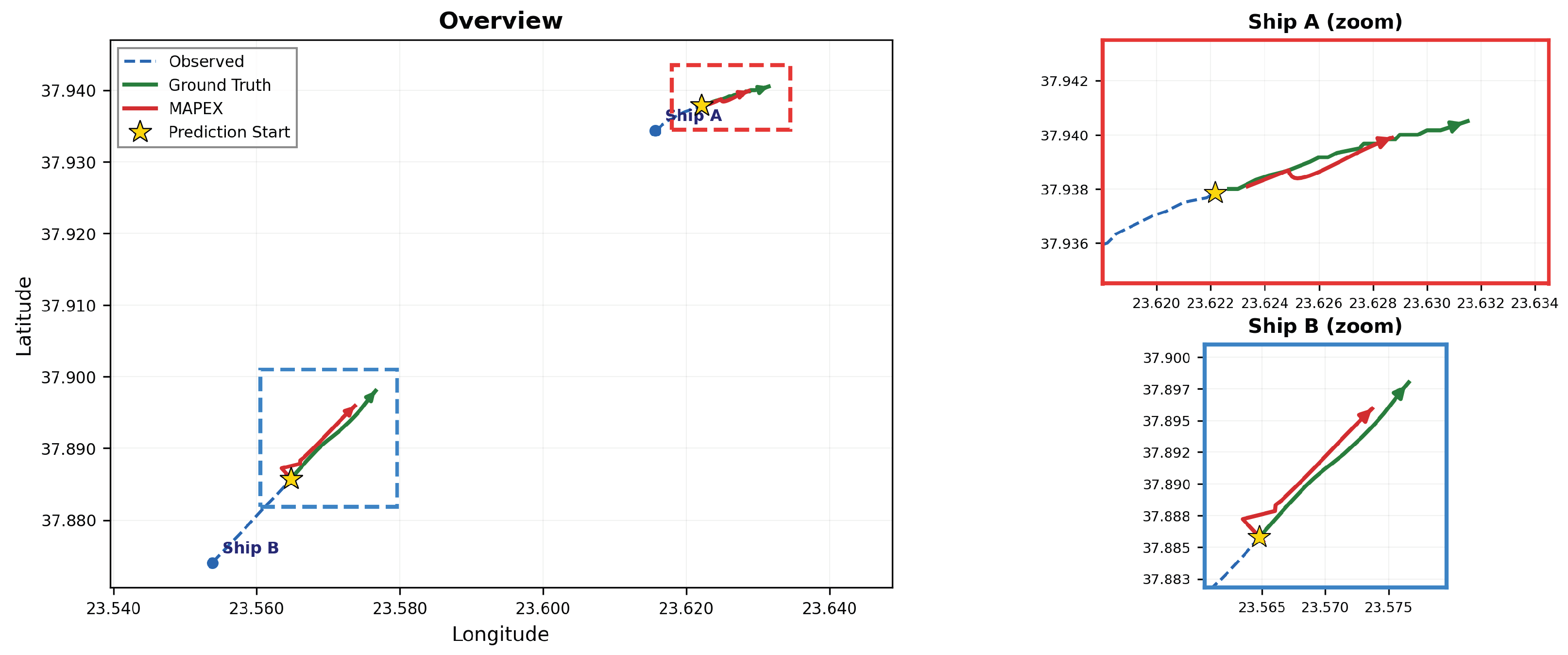
Qualitative prediction results on a pairwise encounter from the Piraeus AIS test set. Left: overview showing the full spatial context with observed trajectories (blue dashed), ground truth future positions (green), and Mapex predictions (red). Right: zoomed views of each vessel’s prediction region. The spatial visualization enables the model to capture both vessels’ trajectories simultaneously from a shared scene representation.
Figure 8.
Qualitative prediction results on a pairwise encounter from the Piraeus AIS test set. Left: overview showing the full spatial context with observed trajectories (blue dashed), ground truth future positions (green), and Mapex predictions (red). Right: zoomed views of each vessel’s prediction region. The spatial visualization enables the model to capture both vessels’ trajectories simultaneously from a shared scene representation.
Table 1.
Piraeus AIS dataset statistics.
Table 1.
Piraeus AIS dataset statistics.
| Property | Value |
|---|
| Region | Piraeus/Saronic Gulf, Greece |
| Period | May 2017–December 2019 |
| Sampling interval | 10 min |
| Latitude range | 37.5– N |
| Longitude range | 23.1– E |
| Observation window (T) | 18 steps (3 h) |
| Prediction horizon (P) | 24 steps (4 h) |
| Encounter detection radius | 5 nm |
| Scene size (N) | 2–8 vessels |
| Train encounters/windows (pairwise) | 2912
/217,159 |
| Validation encounters/windows (pairwise) | 513/36,317 |
| Test encounters/windows (pairwise) | 5000/402,733 |
Table 2.
MMSI-shared vs. MMSI-disjoint diagnostic on the held-out test set, evaluated on the same five-seed-mean Mapex checkpoint. shared: encounters whose vessel MMSIs appear somewhere in the train month. disjoint: encounters whose vessel MMSIs never appear in the train month. No sample, encounter, or trajectory window is shared between train and test; the only thing the shared subset shares with training is vessel identity across months. Both subsets remain substantially below the strongest prior baseline.
Table 2.
MMSI-shared vs. MMSI-disjoint diagnostic on the held-out test set, evaluated on the same five-seed-mean Mapex checkpoint. shared: encounters whose vessel MMSIs appear somewhere in the train month. disjoint: encounters whose vessel MMSIs never appear in the train month. No sample, encounter, or trajectory window is shared between train and test; the only thing the shared subset shares with training is vessel identity across months. Both subsets remain substantially below the strongest prior baseline.
| Test Subset | N Samples | ADE (nm) ↓ | FDE (nm) ↓ |
|---|
| shared (MMSI seen in train month) |
|
|
|
| disjoint (MMSI never seen) |
|
|
|
| Relative gap (disjoint/shared) | — |
|
|
Table 3.
Trajectory prediction performance on the Piraeus AIS held-out test set (October 2017 file; see
Section 6.2). ADE and FDE are in nautical miles (nm); MSE is the summed squared error over the
normalized prediction tensor, matching the aggregation used in [
7]. All
Mapex numbers are reported as mean±std over five random seeds (42–46). Baseline ADE/FDE/MSE for the iTransformer variants and AIS-LLM are quoted as reported in [
7] on the same Piraeus dataset; we reproduce only the TrAISformer baseline on our exact test split (the bottom row, “our re-evaluation”) because its codebase is publicly available and small-model. AIS-LLM is the lowest-error baseline in the original reference and, by our reading, the genuine prior SOTA on this benchmark; we do not re-evaluate it here because it is a billion-parameter LLM (Qwen2-1.5B) with a custom QLoRA fine-tuning and multi-task framework whose training pipeline is not publicly released, so a faithful reproduction was not feasible within this revision cycle. We therefore report two parallel comparisons: against AIS-LLM with its quoted numbers (the SOTA-axis comparison, with the apples-to-apples caveat noted above) and against TrAISformer with our re-evaluated numbers (the apples-to-apples-on-our-split comparison). Both yield ADE reductions in the same ballpark as the abstract’s “approximately
” headline, supporting the claim under either reproducibility regime. This limitation is flagged in the Reviewer 4 response letter. Lower is better. Best in
bold, second best
underlined.
Table 3.
Trajectory prediction performance on the Piraeus AIS held-out test set (October 2017 file; see
Section 6.2). ADE and FDE are in nautical miles (nm); MSE is the summed squared error over the
normalized prediction tensor, matching the aggregation used in [
7]. All
Mapex numbers are reported as mean±std over five random seeds (42–46). Baseline ADE/FDE/MSE for the iTransformer variants and AIS-LLM are quoted as reported in [
7] on the same Piraeus dataset; we reproduce only the TrAISformer baseline on our exact test split (the bottom row, “our re-evaluation”) because its codebase is publicly available and small-model. AIS-LLM is the lowest-error baseline in the original reference and, by our reading, the genuine prior SOTA on this benchmark; we do not re-evaluate it here because it is a billion-parameter LLM (Qwen2-1.5B) with a custom QLoRA fine-tuning and multi-task framework whose training pipeline is not publicly released, so a faithful reproduction was not feasible within this revision cycle. We therefore report two parallel comparisons: against AIS-LLM with its quoted numbers (the SOTA-axis comparison, with the apples-to-apples caveat noted above) and against TrAISformer with our re-evaluated numbers (the apples-to-apples-on-our-split comparison). Both yield ADE reductions in the same ballpark as the abstract’s “approximately
” headline, supporting the claim under either reproducibility regime. This limitation is flagged in the Reviewer 4 response letter. Lower is better. Best in
bold, second best
underlined.
| Model | ADE (nm) ↓ | FDE (nm) ↓ | MSE ↓ |
|---|
| Coordinate-domain baselines
[7] |
| TrAISformer [5] | 0.66 | 1.22 | 268.98 |
| iReformer [6] | 0.52 | 1.12 | 272.16 |
| iFlashformer [6] | 0.50 | 1.11 | 272.16 |
| iTransformer [6] | 0.50 | 1.10 | 272.16 |
| iFlowformer [6] | 0.50 | 1.10 | 272.16 |
| iInformer [6,46] | 0.48 | 1.05 | 272.16 |
| AIS-LLM [7] | 0.43 | 0.91 | 95.76 |
| TrAISformer (our re-evaluation) [5] | 0.486 | 0.636 | — |
| MAPEX (Ours) |
|
|
|
Table 4.
Model complexity comparison. Mapex is larger than coordinate-domain baselines due to the visual encoder but remains orders of magnitude smaller than LLM-based approaches.
Table 4.
Model complexity comparison. Mapex is larger than coordinate-domain baselines due to the visual encoder but remains orders of magnitude smaller than LLM-based approaches.
| Model | Params | Architecture |
|---|
| TrAISformer [5] | ∼10 M+ | Causal Transformer + CE |
| iTransformer [6] | — | Inverted Transformer |
| iInformer [6,46] | — | ProbSparse Attention |
| MAPEX (Ours) | 5.3 M | ViT + Coord + GRU |
| AIS-LLM [7] | ∼3B+ | LLM + Multi-task |
Table 5.
Per-sample inference latency on a single NVIDIA RTX 4090 GPU (pairwise mode, batch size 1, warm start, mean over 500 samples after 50-step warm-up). Rasterization runs on CPU; neural forward passes run on GPU. For Mapex, the Forward (GPU) column reports the combined ViT + coordinate branch + GRU decoder time, not profiled separately because the three blocks share a single forward call. The iInformer row is provided as a coordinate-domain reference; rasterization does not apply because iInformer consumes coordinate vectors directly. iInformer was instantiated with the iTransformer paper’s standard short-horizon configuration (, 4 heads, 2 encoder layers, ) over the same 18-step input and 24-step output window, with 205 K parameters; latency depends on tensor shapes and layer count, not on parameter values, so a fresh-init instance and a trained instance produce statistically equivalent timing.
Table 5.
Per-sample inference latency on a single NVIDIA RTX 4090 GPU (pairwise mode, batch size 1, warm start, mean over 500 samples after 50-step warm-up). Rasterization runs on CPU; neural forward passes run on GPU. For Mapex, the Forward (GPU) column reports the combined ViT + coordinate branch + GRU decoder time, not profiled separately because the three blocks share a single forward call. The iInformer row is provided as a coordinate-domain reference; rasterization does not apply because iInformer consumes coordinate vectors directly. iInformer was instantiated with the iTransformer paper’s standard short-horizon configuration (, 4 heads, 2 encoder layers, ) over the same 18-step input and 24-step output window, with 205 K parameters; latency depends on tensor shapes and layer count, not on parameter values, so a fresh-init instance and a trained instance produce statistically equivalent timing.
| Configuration | Rasterize (ms, CPU) | Forward (ms, GPU) | End-to-End (ms) |
|---|
| Mapex (no cache) |
|
|
|
| Mapex (cached raster) | 0 |
|
|
| iInformer (forward only) | — |
|
|
Table 6.
Ablation study on the Piraeus AIS pairwise test set, reported as 5-seed mean ± std (seeds 42–46). All variants are trained from scratch for 30 epochs with identical hyperparameters. Best in bold; units: nautical miles (nm).
Table 6.
Ablation study on the Piraeus AIS pairwise test set, reported as 5-seed mean ± std (seeds 42–46). All variants are trained from scratch for 30 epochs with identical hyperparameters. Best in bold; units: nautical miles (nm).
| Variant | ADE ↓ | FDE ↓ |
|---|
| MAPEX (full)
|
|
|
| Input channel ablation |
| w/o speed channel |
|
|
| w/o heading channel |
|
|
| Architecture ablation |
| Visual-only (Mapex-V, no coord branch) |
|
|
| Coord-only (Mapex-C, no ViT encoder) |
|
|
| Resolution ablation |
| 64 × 64 |
|
|
Table 7.
Per-channel test-set MSE in normalized output space (
z-scored), 5-seed mean ± std on the Piraeus test split (seeds 42–46). Values are not directly comparable across channels because each channel’s normalization variance differs; within-channel comparison between variants is the informative one. The two angular channels (COG, heading) show MSE roughly two orders of magnitude larger than lat/lon/SOG, consistent with the classical
wraparound penalty incurred when angular state is normalized as a continuous scalar rather than with a circular encoding. Because our headline ADE/FDE in
Table 3 are computed only from lat/lon via the haversine distance, the wraparound penalty inflates training MSE but does not contaminate the reported position metrics; a
re-encoding is flagged as future work (
Section 8).
Table 7.
Per-channel test-set MSE in normalized output space (
z-scored), 5-seed mean ± std on the Piraeus test split (seeds 42–46). Values are not directly comparable across channels because each channel’s normalization variance differs; within-channel comparison between variants is the informative one. The two angular channels (COG, heading) show MSE roughly two orders of magnitude larger than lat/lon/SOG, consistent with the classical
wraparound penalty incurred when angular state is normalized as a continuous scalar rather than with a circular encoding. Because our headline ADE/FDE in
Table 3 are computed only from lat/lon via the haversine distance, the wraparound penalty inflates training MSE but does not contaminate the reported position metrics; a
re-encoding is flagged as future work (
Section 8).
| Channel | Mapex (Full) | Mapex-V (Visual-Only) |
|---|
| lat |
|
|
| lon |
|
|
| SOG |
|
|
| COG |
|
|
| heading |
|
|
Table 8.
Empirical pixel-to-distance distribution computed on a random 20,000-scene subset of the Piraeus test set at the default canvas resolution. Adaptive bbox uses a 20% margin around the N-vessel scene. Values are in meters per pixel (canvas-side resolution).
Table 8.
Empirical pixel-to-distance distribution computed on a random 20,000-scene subset of the Piraeus test set at the default canvas resolution. Adaptive bbox uses a 20% margin around the N-vessel scene. Values are in meters per pixel (canvas-side resolution).
| Statistic over Test Scenes | Pixel Resolution (m/Pixel) |
|---|
| Median | 23.9 |
| Mean | 33.8 |
| IQR (25–75%) | 12.8–55.2 |
| 95th percentile | 71.6 |
Table 9.
Along-track and cross-track displacement errors on the v2 MMSI-strict test split, seed 42. Mean over
predicted trajectories; per-sample standard deviation in parentheses. We report a single seed here because the purpose of the v2 MMSI-strict protocol in this paper is to establish the relative margin over baselines under strict vessel disjointness (see
Section 6.2); the 5-seed protocol is applied to the v1 headline numbers in
Table 3.
Table 9.
Along-track and cross-track displacement errors on the v2 MMSI-strict test split, seed 42. Mean over
predicted trajectories; per-sample standard deviation in parentheses. We report a single seed here because the purpose of the v2 MMSI-strict protocol in this paper is to establish the relative margin over baselines under strict vessel disjointness (see
Section 6.2); the 5-seed protocol is applied to the v1 headline numbers in
Table 3.
| Component | ADE (nm) ↓ | FDE (nm) ↓ |
|---|
| Total (haversine) | () | () |
| Along-track (reach) | () | () |
| Cross-track | () | () |
Table 10.
ADE per condition subset on the v2 MMSI-strict test split, seed 42. Bins are mutually exclusive subsets of the test samples; n is the number of samples in each.
Table 10.
ADE per condition subset on the v2 MMSI-strict test split, seed 42. Bins are mutually exclusive subsets of the test samples; n is the number of samples in each.
| Stratification | Bin | ADE (nm) ↓ | n |
|---|
| Speed (SOG) | slow kn |
|
|
| | medium 5–15 kn |
|
|
| | fast kn |
|
|
| Scene bbox | compact nm |
|
|
| | moderate 5–15 nm |
|
|
| | wide nm | — | 0 |
| Inter-ship dist | close nm |
|
|
| | medium 1–3 nm |
|
|
| | far nm |
|
|
Table 11.
Operational metrics for Mapex (full) vs. Mapex-V (visual-only) on the Piraeus v1 test set, seed 42. CPA error is in nautical miles (nm). COLREGs accuracy is the fraction of encounters whose four-class encounter type at TCPA agrees with the ground-truth label. “All” covers every pairwise encounter (); the close-encounter subset filters to ground-truth CPA nm ().
Table 11.
Operational metrics for Mapex (full) vs. Mapex-V (visual-only) on the Piraeus v1 test set, seed 42. CPA error is in nautical miles (nm). COLREGs accuracy is the fraction of encounters whose four-class encounter type at TCPA agrees with the ground-truth label. “All” covers every pairwise encounter (); the close-encounter subset filters to ground-truth CPA nm ().
| Subset | Metric | Mapex | Mapex-V |
|
|---|
| All | CPA error mean (nm) ↓ |
| 0.164 |
|
| TCPA error mean (steps) ↓ |
|
|
|
| COLREGs accuracy ↑ |
|
|
|
| Near-miss detection ↑ |
|
|
|
| Close, CPA < 1 nm | CPA error mean (nm) ↓ |
|
|
|
| TCPA error mean (steps) ↓ |
|
|
|
| COLREGs accuracy↑ |
|
|
|
| Near-miss detection ↑ |
|
|
|
Table 12.
Pairwise Mapex accuracy stratified by ambient scene size on the Piraeus v1 test month. Each prediction is a per-vessel forecast inside a pair; the scene size N is the number of vessels co-located at the encounter time. Piraeus traffic is sparse, so does not occur with meaningful frequency in the natural distribution; this is a property of the dataset, not of the architecture.
Table 12.
Pairwise Mapex accuracy stratified by ambient scene size on the Piraeus v1 test month. Each prediction is a per-vessel forecast inside a pair; the scene size N is the number of vessels co-located at the encounter time. Piraeus traffic is sparse, so does not occur with meaningful frequency in the natural distribution; this is a property of the dataset, not of the architecture.
| Scene Size N | n Predictions | ADE (nm) ↓ | FDE (nm) ↓ |
|---|
| 2 |
|
|
|
| 3 |
|
|
|
| 4 | 8688 | 0.096 |
|
Table 13.
Cross-port retraining experiments on NOAA MarineCadastre 2022. Both Mapex and TrAISformer are trained from scratch on the same MMSI-strict split per port (vessels disjoint between train and test). LA = Los Angeles/Long Beach; SF = San Francisco Bay. Sample counts: LA pairwise train /TrAISformer per-trajectory test 140; SF pairwise train /per-trajectory test 114. ADE/FDE in nautical miles, seed 42. TrAISformer scores are min-of-16 sampling, the more favorable scoring regime for that model.
Table 13.
Cross-port retraining experiments on NOAA MarineCadastre 2022. Both Mapex and TrAISformer are trained from scratch on the same MMSI-strict split per port (vessels disjoint between train and test). LA = Los Angeles/Long Beach; SF = San Francisco Bay. Sample counts: LA pairwise train /TrAISformer per-trajectory test 140; SF pairwise train /per-trajectory test 114. ADE/FDE in nautical miles, seed 42. TrAISformer scores are min-of-16 sampling, the more favorable scoring regime for that model.
| Variant/Corpus | ADE (nm) ↓ | FDE (nm) ↓ | n Test |
|---|
| Mapex (full), LA |
|
| 687 |
| Mapex-V, LA |
|
| 687 |
| TrAISformer, LA |
|
| 140 |
| Mapex (full), SF |
|
| 709 |
| Mapex-V, SF |
|
| 709 |
| TrAISformer, SF |
|
| 114 |