Article

MAPEX: Map Exploitation for Vision-Based Ship Trajectory Prediction

College of Economics and Business, Hankuk University of Foreign Studies, 81, Oedae-ro, Mohyeon-eup, Cheoin-gu, Yongin-si 17035, Gyeonggi-do, Republic of Korea
*
Author to whom correspondence should be addressed.
Systems 2026, 14(5), 536; https://doi.org/10.3390/systems14050536
Submission received: 22 March 2026 / Revised: 5 May 2026 / Accepted: 7 May 2026 / Published: 8 May 2026

Abstract

Ship trajectory prediction from Automatic Identification System (AIS) data has been predominantly approached as a time-series forecasting problem, where sequential models operate on coordinate sequences to predict future positions. This paradigm, while effective, neglects a key observation: the spatial layout of multiple vessel trajectories on a chart-like plane carries rich interaction information that is difficult to capture through sequential processing alone. To address this, Mapex (Map Exploitation) is proposed as a vision-based framework that rasterizes multi-vessel AIS trajectories into chart-like multi-channel images and processes them with a visual encoder, treating trajectory prediction as a map-reading task. Each vessel contributes three image channels encoding its trajectory heatmap, speed field, and heading field, converting raw coordinates into a spatial representation where physical movement patterns become visually apparent. A parallel coordinate branch supplies the course-over-ground information that the raster does not encode explicitly, and a fusion module combines both streams for autoregressive five-channel trajectory generation. Unlike coordinate-domain models that process position sequences numerically, Mapex understands vessel motion through its spatial layout, capturing relative positions, trajectory shapes, and kinematic patterns as visual features rather than abstract number sequences. Experiments on the Piraeus AIS dataset demonstrate that Mapex reduces the average displacement error (ADE) by approximately  68 %  compared to the best coordinate-domain baseline and the mean squared error (MSE) by over  80 %  compared to the strongest prior method, while requiring significantly fewer parameters than recent LLM-based approaches. These results suggest that spatial visualization of trajectories provides a fundamentally richer representation than coordinate sequences for multi-vessel trajectory prediction.

Graphical Abstract

1. Introduction

Maritime trajectory prediction is a cornerstone of vessel traffic management, collision avoidance, and maritime situational awareness. The Automatic Identification System (AIS) broadcasts vessel state information, including latitude, longitude, speed over ground (SOG), course over ground (COG), and heading, at regular intervals, providing the data foundation for trajectory prediction systems. As maritime traffic volumes continue to grow, accurate multi-vessel trajectory prediction becomes increasingly critical for port operations and open-sea navigation safety. Recent studies on collision risk assessment using AIS data [1] and causation analysis of marine traffic accidents [2] further underscore the importance of reliable trajectory prediction as a foundational component for maritime safety systems.
The dominant paradigm for AIS-based trajectory prediction treats the problem as time-series forecasting. Recurrent neural networks [3,4], Transformer architectures [5,6], and more recently Large Language Models [7] process coordinate sequences to predict future positions. Domain-specific approaches further incorporate maritime regulations (COLREGs) [8] through explicit rule encoding, role decomposition, and specialized expert networks.
While these methods have achieved impressive results, they all share a fundamental limitation: they operate exclusively in the coordinate domain, processing trajectories as ordered sequences of numerical values. In this representation, multi-vessel spatial relationships, such as relative positions, convergence angles, and closing speeds, must be inferred through learned arithmetic over abstract number sequences. This places a significant burden on the model, as interaction patterns between vessels lack any explicit spatial structure in the input representation. Moreover, the coordinate-domain paradigm processes each vessel’s state vector independently or through pairwise comparisons, making it difficult to capture holistic scene-level dynamics that emerge from the simultaneous movement of multiple vessels.
We observe that human navigators approach this problem in a fundamentally different manner. When examining a radar display or an electronic chart, a navigator does not process individual coordinate tuples sequentially. Instead, they perceive the spatial layout of vessel tracks on a two-dimensional plane, recognizing relative positions, converging or diverging trajectories, and speeds indicated by track spacing, to form an intuitive understanding of both spatial configuration and movement dynamics. This “map-reading” ability is a spatial pattern recognition task that coordinate-domain models cannot replicate.
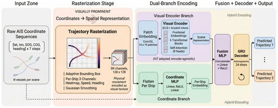
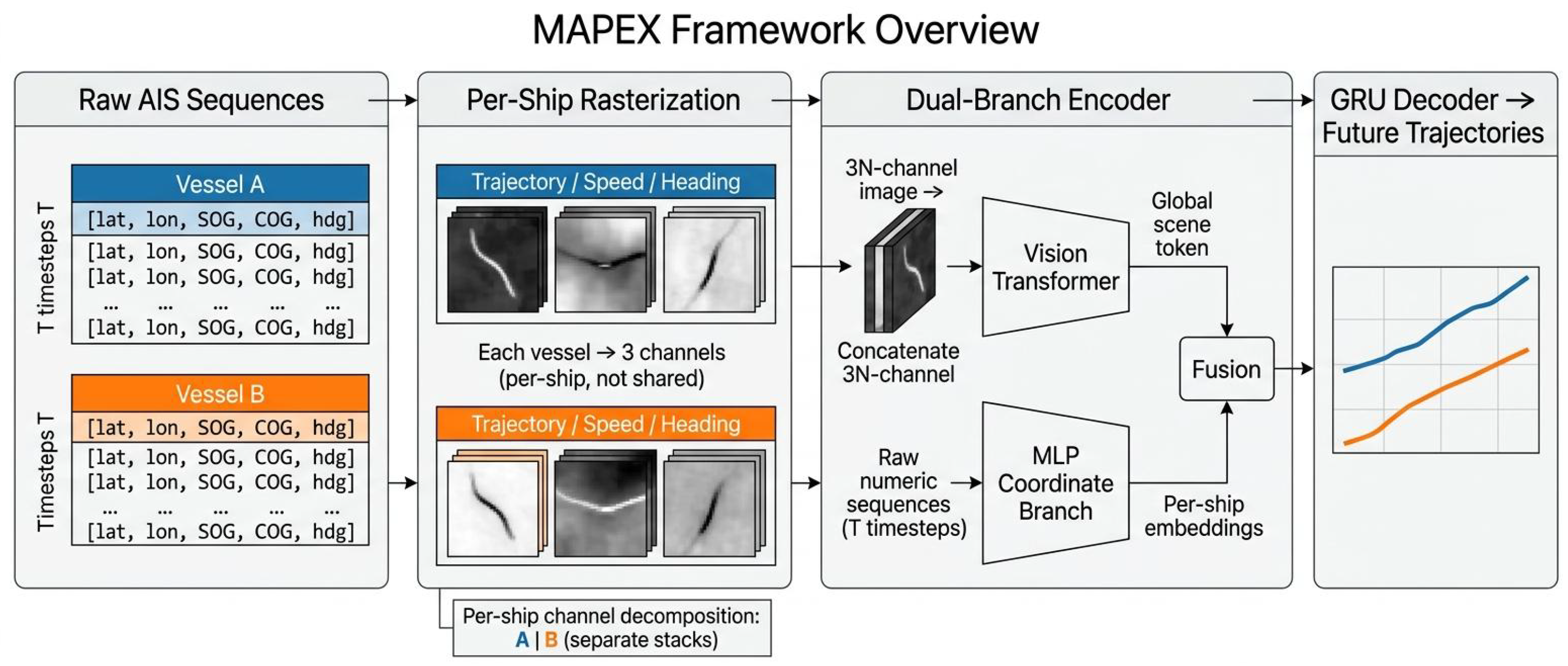
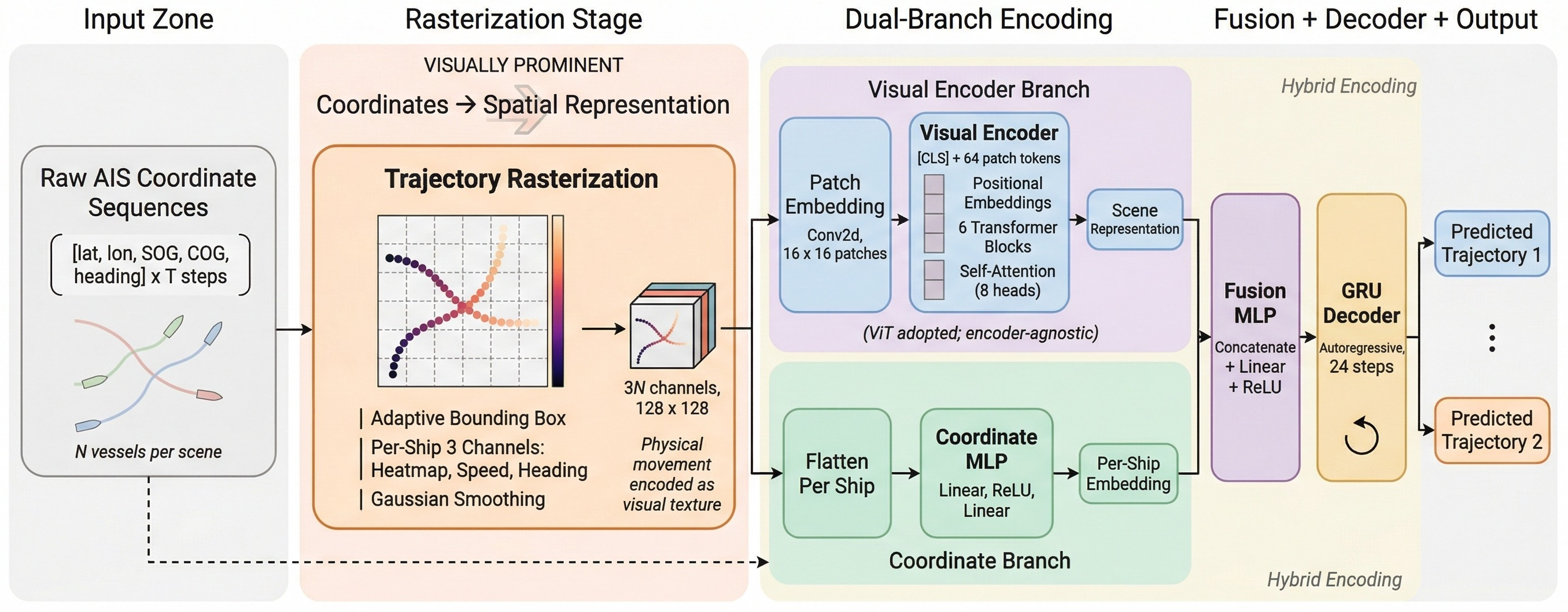
This observation motivates Mapex (Map Exploitation), which reframes maritime trajectory prediction as a spatial understanding problem through visual reconstruction of trajectory data (Figure 1). Our key insight is that by rasterizing multi-vessel AIS trajectories into  128 × 128  multi-channel images analogous to chart overlays, we transform abstract coordinate sequences into a spatial visual representation where both scene-level spatial awareness and vessel-level movement dynamics become directly observable. Each vessel contributes three image channels encoding its trajectory heatmap, speed field, and heading field. In this rasterized representation, spatial relationships that coordinate-domain models must laboriously compute become visually self-evident: converging trajectories appear as lines approaching each other, speed differentials manifest as differences in track density, and heading changes are visible as trajectory curvature. A visual encoder (we adopt a Vision Transformer) processes these images to extract a global scene representation that captures both the spatial configuration and the dynamics of the entire multi-vessel encounter simultaneously. A parallel coordinate branch supplies the course-over-ground information that the raster does not encode explicitly, and a fusion module combines both streams to produce the complete five-channel kinematic output.
This work makes several contributions. We design a trajectory rasterization pipeline that converts raw AIS coordinate sequences into multi-channel images encoding per-vessel trajectory heatmaps, speed fields, and heading fields, enabling spatial awareness and dynamics understanding through visual reconstruction rather than numerical processing. We demonstrate that this visual representation captures spatial relationships and kinematic patterns that coordinate-domain models struggle to extract from number sequences, achieving substantially better prediction accuracy with a simple encoder-decoder architecture and pure MSE loss, without domain-specific modules. A hybrid architecture combines a visual encoder with a parallel coordinate branch that supplies the course-over-ground channel the raster does not encode, and the framework scales naturally to multi-vessel encounters by simply adding image channels.

2. Related Work

2.1. Deep Learning for Vessel Trajectory Prediction

Deep learning has become the dominant paradigm for vessel trajectory prediction. Gao et al. [3] pioneered LSTM-based ship trajectory prediction, demonstrating that recurrent architectures effectively capture temporal dependencies in vessel motion. Park et al. [4] extended this with bi-directional LSTMs that exploit both past and future context during training. Murray and Perera [9] proposed a multi-modal deep-learning approach fusing multiple AIS feature channels. Li et al. [10] provided a comprehensive benchmarking of ML and DL methods for AIS-driven trajectory prediction, establishing key performance baselines. TrAISformer [5] introduced a Transformer architecture with sparse augmented data representation for AIS trajectory prediction. Zhang et al. [11] surveyed GAN-based approaches for generating diverse plausible trajectories, and a related line of work [12] explored graph neural networks for modeling spatial relationships among multiple vessels. AIS-LLM [7] proposed a unified LLM-based framework for multi-task maritime analysis including trajectory prediction, achieving strong results but requiring billions of parameters. More recently, rule-aware approaches have incorporated COLREGs [8] compliance through explicit geometric feature extraction, situation classification, and role-conditioned decoding, demonstrating that domain knowledge can substantially improve prediction accuracy.
All of these approaches operate in the coordinate domain, processing trajectories as numerical sequences. Mapex departs from this paradigm by converting trajectories into images and applying vision-based processing.

2.2. Vision Transformers

The Transformer architecture [13] has revolutionized sequence modeling across domains. The Vision Transformer (ViT) [14] demonstrated that pure Transformer architectures, when applied to sequences of image patches, can match or exceed convolutional neural networks on image classification. ViT divides an image into fixed-size patches, projects them to embeddings, and processes the resulting sequence with standard Transformer blocks. A learnable CLS token aggregates global information through self-attention.
DeiT [15] introduced data-efficient training strategies and knowledge distillation for ViT, enabling competitive performance with less data. Swin Transformer [16] proposed hierarchical feature maps and shifted window attention for improved efficiency and multi-scale representation. BEiT [17] adapted BERT-style pre-training to vision through masked image modeling. V-MoE [18] applied sparse Mixture-of-Experts to ViT, demonstrating that conditional computation can scale vision models efficiently.
In the trajectory prediction domain, Cheng et al. [19] proposed Vit-Traj, a spatial–temporal coupling vehicle trajectory prediction model that uses 2D convolutions to extract spatio-temporal features from coordinate tensors and employs ViT for feature fusion. While Vit-Traj demonstrates the effectiveness of ViT in trajectory prediction, it processes raw coordinate tensors rather than spatial visual representations. In their framework, the ViT serves as a feature fusion module for abstract feature maps extracted by CNNs, rather than as a visual encoder that reads spatial patterns from rasterized images. In contrast, Mapex rasterizes trajectories into actual chart-like images where physical movement patterns are directly visible, enabling the ViT to leverage its spatial reasoning capabilities on genuine visual content. This distinction is fundamental: Mapex’s core contribution lies in the rasterization representation itself, not merely the choice of encoder architecture.
Mapex adopts ViT as its visual encoder for processing rasterized trajectory images. The choice of encoder is secondary to the core contribution, which is the spatial representation itself, though the self-attention mechanism across image patches is well-suited for reasoning about spatial relationships between vessel trajectories at different locations in the scene.

2.3. Image-Based Trajectory Prediction

The idea of using spatial representations for trajectory prediction has been extensively explored in the pedestrian and multi-agent domains. The Social Force model [20] pioneered physics-based spatial interaction modeling for pedestrian dynamics. Social LSTM [21] introduced social pooling layers that aggregate neighboring agents’ hidden states based on spatial proximity. Social-STGCNN [22] extended this with spatio-temporal graph convolutions, modeling interactions as graph edges. SoPhie [23] combined social attention with physical constraints using scene images for path prediction. Trajectron++ [24] proposed a graph-structured approach that incorporates scene context through rasterized maps for dynamically-feasible trajectory forecasting. PECNet [25] introduced endpoint-conditioned prediction that reasons about spatial goal locations. AgentFormer [26] applied agent-aware Transformers to multi-agent forecasting, and EqMotion [27] leveraged equivariant neural networks for interaction-aware multi-agent prediction.
These works demonstrate that spatial/visual representations can capture interaction patterns that are difficult to model in pure coordinate space. However, they have not been applied to the maritime domain, where the scale of interactions (nautical miles rather than meters), the kinematic constraints of large vessels, and the regulatory framework (COLREGs) create fundamentally different challenges. Mapex bridges this gap by adapting the rasterization paradigm to maritime AIS data.

2.4. Rasterization and Spatial Encoding in Transportation

In autonomous driving, rasterized bird’s-eye view (BEV) representations have become a dominant paradigm for multi-agent prediction and planning. ChauffeurNet [28] pioneered the use of rasterized top-down scene representations as input for end-to-end driving policies via imitation learning. Cui et al. [29] applied rasterized BEV images with deep CNNs for multimodal trajectory prediction. CoverNet [30] formulated behavior prediction as classification over a fixed set of trajectory anchors from rasterized scenes. Djuric et al. [31] extended rasterized prediction with calibrated uncertainty estimation for short-term motion forecasting. BEVFormer [32] learns BEV representations from multi-camera images via spatio-temporal Transformers. Lift-Splat-Shoot (LSS) [33] encodes camera images into a BEV grid through explicit depth estimation. PointPillars [34] rasterizes LiDAR point clouds into a pillar-based BEV representation for efficient 3D object detection. CenterPoint [35] demonstrates center-based detection and tracking from BEV representations, highlighting the effectiveness of rasterized spatial encoding for multi-agent reasoning. Scene Transformer [36] unified multi-agent prediction through a joint Transformer architecture operating on spatial scene representations.
These approaches demonstrate that converting spatial data into image-like representations enables powerful visual reasoning about multi-agent dynamics. Mapex applies an analogous principle to maritime trajectory prediction: by rasterizing AIS trajectories into chart-like images, we enable spatial reasoning about vessel interactions through the same visual representation mechanisms that have proven effective in autonomous driving.

2.5. Broader Context: Spatio-Temporal Forecasting and Maritime Analytics

A wider body of spatio-temporal forecasting research situates Mapex within two complementary currents that have so far progressed largely in parallel. The first current concerns spatio-temporal deep learning in the earth and climate sciences, where forecasts are typically defined over a spatial grid rather than as per-agent sequences. Xu et al. [37] survey this field and emphasize that grid-structured, image-like representations have become the de facto input format because they expose spatial correlations directly to convolutional and attention-based backbones; they also highlight uncertainty quantification as a critical but still under-developed dimension of such forecasts. Building on that observation, Xu et al. [38] show that deterministic precipitation predictors can be upgraded to calibrated distributions by jointly modeling data and model uncertainty within a probabilistic deep-learning encoder–decoder. Mapex inherits the first lesson, namely that spatial grids are a natural substrate for multi-agent reasoning, while remaining deterministic in the present work; the probabilistic extensions suggested by this literature indicate a clear future direction for quantifying predictive uncertainty in dense maritime encounters.
The second current concerns macro-scale maritime analytics built on AIS data. Container-shipping carbon-emission forecasting [39] aggregates AIS trajectories into regional or route-level flow statistics to predict emissions at port or fleet granularity, whereas port-area traffic-flow prediction [40] couples graph theory with time-series models to forecast arrival intensities and queueing dynamics. These approaches solve complementary problems at a coarser temporal and spatial aggregation than Mapex: they consume aggregated AIS signals to forecast throughput or emissions, whereas Mapex predicts per-vessel future tracks that could in principle serve as the micro-level input to such macro forecasters. Our spatial-visual formulation is also conceptually adjacent to the graph-theoretic port models of [40], since both emphasize relational structure among vessels, but differs in that graph models commit to an explicit node–edge topology whereas Mapex lets a ViT learn relational structure implicitly from the rasterized scene. Together, these two currents position Mapex as a vessel-level, grid-encoded spatio-temporal predictor that bridges the micro–macro gap and is naturally composable with uncertainty-aware and aggregation-level methods.

3. Problem Formulation

Consider a maritime scene involving N vessels ( 2 N 8 ). Each vessel i has an observed trajectory  H i = [ x i 1 , , x i T ]  where  x i t = [ lat , lon , SOG , COG , heading ] t R 5 , and we maintain the raw (unnormalized) trajectory  R i  for the rasterization pipeline. The ground-truth future trajectory of vessel i over the prediction horizon is denoted  Y i = [ x i T + 1 , , x i T + P ] , where each future state  x i t R 5  shares the same feature dimension as the observed states. The model’s prediction for the same horizon is denoted  Y ^ i = [ x ^ i ( 1 ) , , x ^ i ( P ) ] R P × 5 , and accuracy is evaluated primarily on the two positional components (latitude and longitude).
Task: Given  { H i , R i } i = 1 N  over T observation steps (default:  T = 18 , i.e., 3 h at 10-min intervals), predict all vessels’ future trajectories  { Y ^ i } i = 1 N  over P prediction steps (default:  P = 24 , i.e., 4 h).
Unlike coordinate-domain approaches that process vessel states as numerical sequences, Mapex treats this as a spatial understanding problem. By rasterizing trajectories into visual representations, spatial relationships and physical movement patterns become directly observable features, enabling the model to learn interaction behaviors from spatial patterns rather than from abstract numerical sequences.

4. Proposed Method: MAPEX

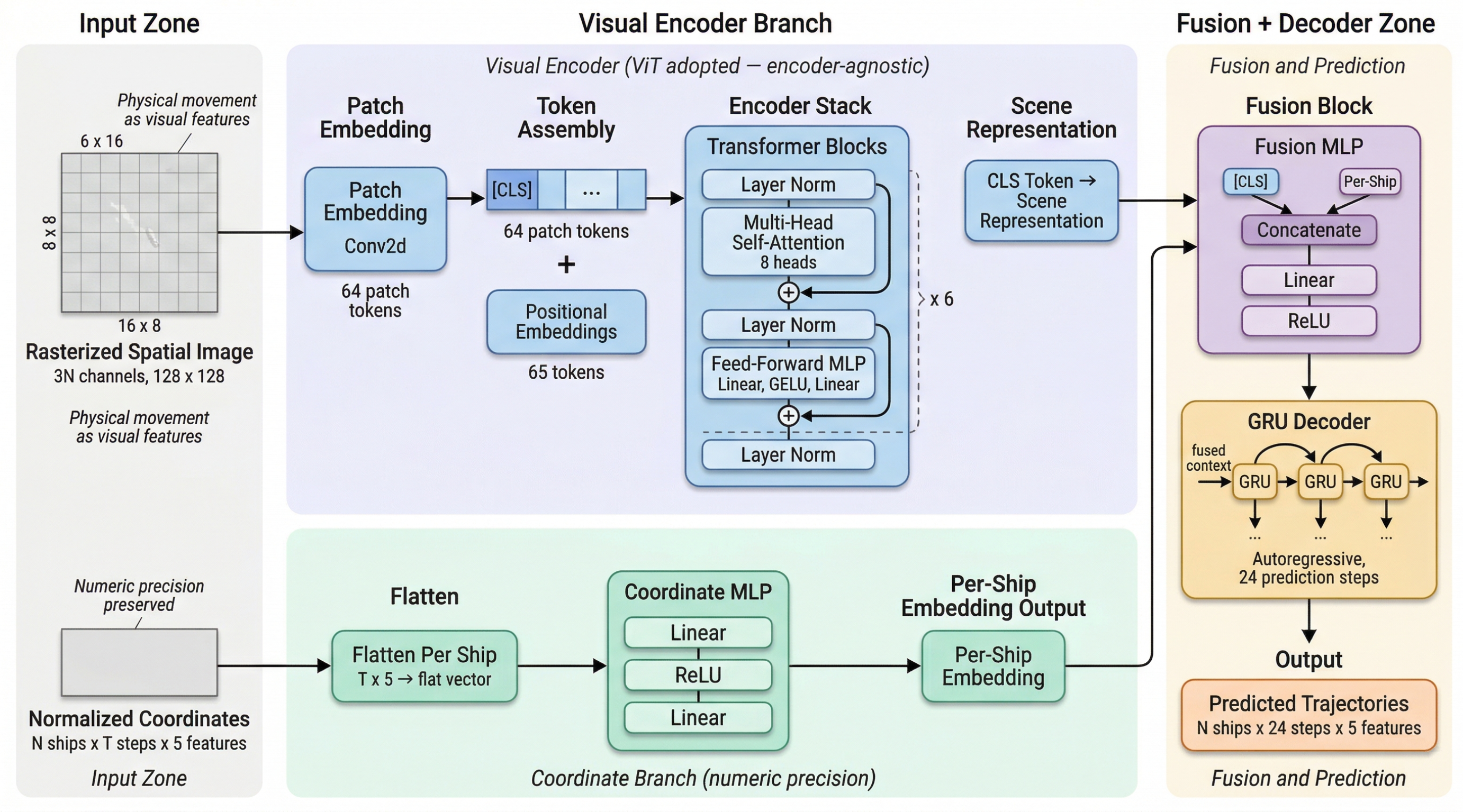
Mapex consists of four components: (1) a trajectory rasterization pipeline that converts AIS coordinates into multi-channel images, (2) a Vision Transformer encoder that extracts global scene representations, (3) a coordinate branch that supplies the course-over-ground information the raster does not encode, and (4) a fusion module and GRU decoder for five-channel trajectory generation. Figure 1 provides an overview and Figure 2 details the architecture.

4.1. Trajectory Rasterization

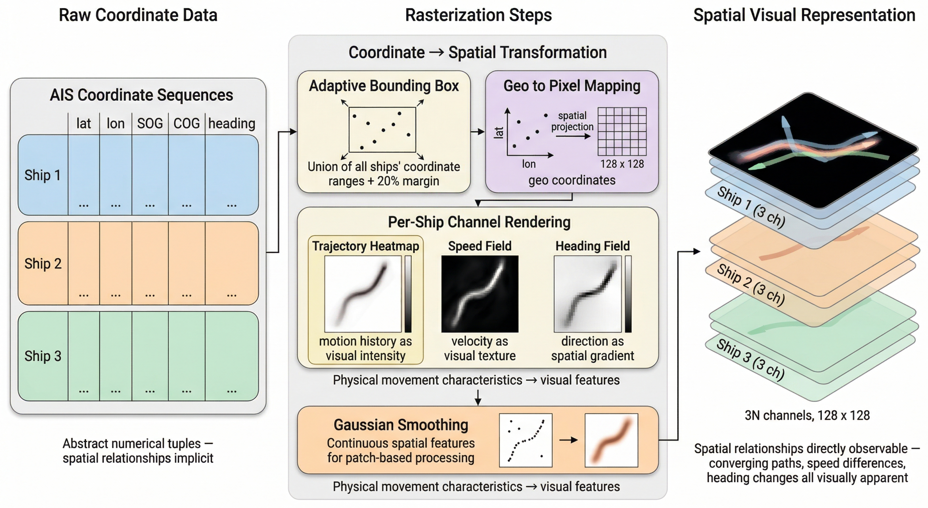
The rasterization pipeline converts raw AIS coordinates into a  C × H × W  image tensor, where  C = 3 N  (three channels per vessel) and  H = W = 128 . Each vessel contributes three channels that encode complementary aspects of its trajectory. All N vessels in a scene are rendered onto a single shared  H × W  canvas with one common adaptive bounding box, rather than into per-vessel sub-images that are later concatenated; the per-vessel decomposition is along the channel axis only. As a result, every pair of vessels is co-registered pixel-for-pixel, so a  0.1  nm close passage and a 3 nm separation are encoded as visibly different geometric configurations on the same canvas, and the ViT can attend across vessel-channel groups at the same spatial location to read off relative geometry. Because the bounding box is fitted to the union of all vessels’ positions rather than per-vessel, a slow vessel covering a small area and a fast vessel sweeping across the scene share the same coordinate frame, so the visual representation preserves their relative speed and spatial coverage rather than collapsing them to comparable footprints.
Given all vessels’ raw coordinates  { ( lon i t , lat i t ) } i = 1 N  for  t = 1 , , T , we first compute an adaptive bounding box by determining the spatial extent and adding a 20% margin:
lon min / max = min / max ( lon i t ) / ± 0.2 · Δ lon lat min / max = min / max ( lat i t ) / ± 0.2 · Δ lat
where  Δ lon = lon max lon min  and similarly for latitude. This margin ensures that trajectories near the boundary have sufficient context and prevents edge artifacts during convolution. Each coordinate is then mapped to pixel space via:
p x = lon lon min lon max lon min · ( W 1 ) p y = lat lat min lat max lat min · ( H 1 )
The rasterized image encodes three channels per vessel. The first channel renders the trajectory as a polyline on a  128 × 128  canvas using Bresenham line drawing between consecutive pixel coordinates, with pixel intensities encoding a temporal gradient  v ( t ) = t / T  so that recent positions appear brighter than earlier ones. This temporal encoding enables the model to infer direction of travel and acceleration patterns from the intensity gradient alone, and the rendered trajectory is smoothed with a Gaussian kernel ( σ = 1.5 ) to produce continuous, anti-aliased lines amenable to the ViT’s patch embedding. The second channel encodes the speed field: each pixel along the trajectory is assigned the normalized SOG at the corresponding timestep,  v speed ( t ) = SOG i t / SOG max , allowing the model to distinguish between fast-moving and stationary vessels. The third channel records the heading field, with each pixel encoding the vessel’s heading normalized to  [ 0 ,   1 ]  as  v hdg ( t ) = heading i t / 360 ; combined with the trajectory heatmap, this enables the model to assess directional state, which is critical for predicting turns and course changes.
The choice of heading (HDG) over course over ground (COG) for the angular channel is deliberate: HDG reflects the vessel’s intended bow direction, set by the rudder and reported by the compass, whereas COG is the realized motion direction that already incorporates drift, wind, and current. At the 10-min AIS sampling interval used here, HDG and COG diverge most when a vessel is maneuvering or being pushed by current, exactly the regime in which knowing what the crew is trying to do carries more predictive signal than knowing what has already been drifted. Mapex does not lose access to COG: the coordinate branch (Section 4.3) consumes the full 5-tuple  ( lat , lon , SOG , COG , HDG )  at every step, so the image plane prioritizes the intent-carrying channel while the coordinate branch retains the outcome-carrying one.
The resulting image  I R 3 N × 128 × 128  contains all observable information about the multi-vessel scene in a format amenable to visual processing. Figure 3 illustrates the rasterization pipeline for a sample encounter.
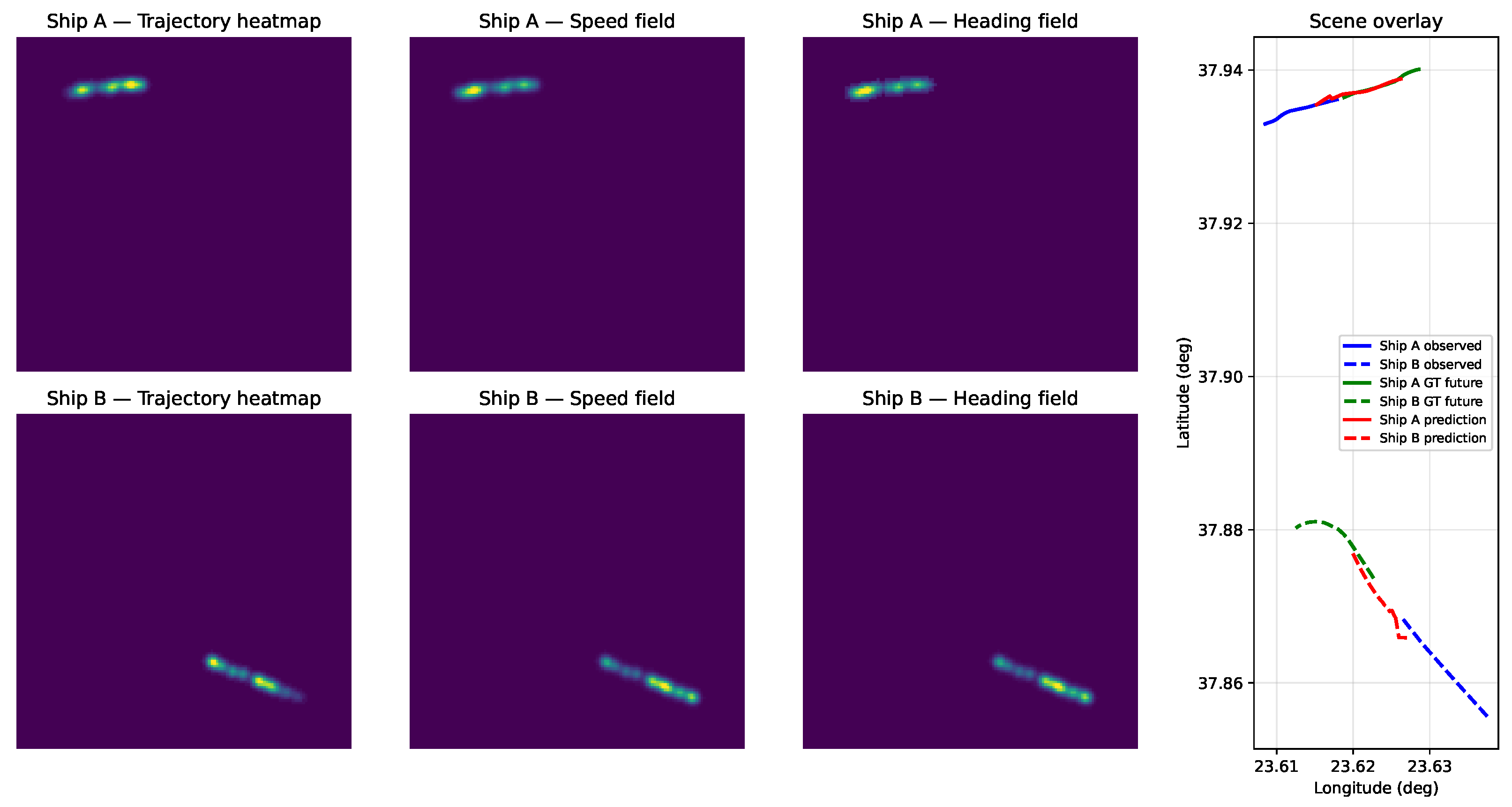
Figure 4 shows the rasterization pipeline applied to a real test-set encounter, displaying the actual rendered channels alongside the model’s prediction and per-step error, complementing the schematic in Figure 3.

4.2. Vision Transformer Encoder

The rasterized image is processed by a visual encoder; we adopt a Vision Transformer (ViT) [14] for its ability to capture global spatial relationships through self-attention across image patches. A convolutional layer (Conv2d with kernel size  16 × 16 , stride 16) divides the  128 × 128  image into a grid of  8 × 8 = 64  non-overlapping patches, each projected to a  d = 256 -dimensional embedding:
E = Conv 2 d ( I ) R 64 × 256
The input channel count is set to  3 N  to accommodate variable numbers of vessels (6 channels in pairwise mode, up to 24 in scene mode). A learnable CLS token  e cls R 256  is prepended to the patch sequence, and learnable positional embeddings  P R 65 × 256  are added:
Z ( 0 ) = [ e cls ; E ] + P R 65 × 256
The sequence then passes through  L = 6  Transformer blocks, each consisting of multi-head self-attention (MHSA) and a feed-forward network (FFN) with pre-norm residual connections:
Z ( ) = MHSA ( LN ( Z ( 1 ) ) ) + Z ( 1 ) Z ( ) = FFN ( LN ( Z ( ) ) ) + Z ( )
where LN denotes LayerNorm, MHSA uses 8 attention heads ( d head = 32 ), and the FFN has an expansion ratio of 4 (hidden dimension 1024) with GELU activation and dropout  0.1 . The CLS token from the final block serves as the global scene representation  h scene = Z ( L ) [ 0 ] R 256 , aggregating information from all patches through 6 layers of self-attention to capture both local trajectory details and global spatial relationships among vessels.

4.3. Coordinate Branch

Rasterizing a continuous trajectory onto a finite-resolution multi-channel image incurs a structural information loss that no choice of pixel resolution can eliminate, and the loss is not uniform across kinematic channels. Latitude/longitude are encoded in the trajectory heatmap, speed-over-ground in the speed field, and heading in the heading field; Mapex however outputs a complete five-channel kinematic sequence whose fifth channel, course-over-ground (COG), is the realized motion direction (heading combined with drift and current) and is not rastered. The visual encoder therefore has no pathway to recover COG at float precision, and any model that consumed only the raster would be structurally unable to satisfy the five-channel output specification. The coordinate branch is included in the architecture to carry the full numerical trajectory at float precision and supply the decoder with an explicit representation of the 18-step history, which the ablation in Section 6.6 shows functions empirically as a channel-specific pathway: the branch’s measurable contribution concentrates in COG prediction, while the position channels (lat/lon/SOG) are already well served by the raster alone. We describe this division of labor as observed rather than causally proven; an ablation that further restricts the branch’s input to COG-only is a natural next step left for future work.
For each vessel i, the normalized observation trajectory  H i R T × 5  is flattened to a vector  h i flat R T · 5  (with  T = 18 , this is 90 dimensions) and passed through a two-layer MLP:
e i coord = MLP ( h i flat ) = W 2 · GELU ( W 1 h i flat + b 1 ) + b 2
where  W 1 R 128 × 90 W 2 R 128 × 128 , producing a per-ship coordinate embedding  e i coord R 128 .
This branch operates with shared weights across all vessels, ensuring consistent encoding regardless of vessel identity. The resulting per-vessel embedding gives the downstream decoder explicit access to the numerical COG and heading histories that the visual encoder cannot reconstruct from the raster alone. Section 6.6 quantifies this asymmetric division of labor, and Section 7 revisits the resulting position-vs-COG trade-off that motivates reporting the full configuration as the primary model while transparently noting the visual-only variant for position-focused applications.

4.4. Fusion and GRU Decoder

The fusion module combines the global scene representation from the ViT with per-ship coordinate embeddings to produce a context vector for each vessel. For each vessel i, the ViT CLS token (shared across all vessels) is concatenated with the per-ship coordinate embedding and projected through a fusion MLP:
c i = MLP fuse ( [ h scene e i coord ] ) R 128
where  MLP fuse  maps from  256 + 128 = 384  dimensions to 128 dimensions through two linear layers with a GELU activation in between (widths  384 128 128 ). The resulting context vector  c i  encodes both the global scene understanding and the precise numeric state of vessel i.
Each vessel’s future trajectory is then predicted autoregressively using a GRU decoder [41]. At each prediction step  p = 1 , , P :
h i ( p ) = GRUCell ( [ x ^ i ( p 1 ) c i ] , h i ( p 1 ) ) x ^ i ( p ) = W out h i ( p ) + b out
where  x ^ i ( 0 ) = x i T  (the last observed state),  h i ( 0 ) = c i , the GRUCell has input size  5 + 128 = 133  and hidden size 128, and  W out R 5 × 128  maps the hidden state to the 5-dimensional output space.
The decoder iterates for  P = 24  steps, producing the complete predicted trajectory  Y ^ i = [ x ^ i ( 1 ) , , x ^ i ( P ) ] R P × 5 . For multi-vessel scenes with variable ship count, a boolean mask zeros out predictions for padding vessels, ensuring that the loss computation considers only valid trajectories.

5. Training Objective

Mapex employs a straightforward training objective: mean squared error (MSE) over all five predicted features across the prediction horizon, without any auxiliary losses.
L = 1 N · P i = 1 N p = 1 P x ^ i ( p ) x i ( p ) 2 2
where N is the number of valid (non-padding) vessels in the scene and  P = 24  is the prediction horizon.
The deliberate simplicity of this loss function is a design choice that highlights the core thesis of Mapex: by converting trajectories into spatial visual representations, the rasterized image provides a sufficiently rich input for the model to learn complex interaction patterns, including collision avoidance behaviors, purely from data, without requiring domain-specific loss terms or specialized architectural modules.
The model is optimized using AdamW with a learning rate of  3 × 10 4  and weight decay  10 4 . The learning rate follows a linear warmup schedule over the first 5 epochs, followed by cosine annealing decay to  10 6 , and gradient norms are clipped to 1.0 to stabilize early training when the ViT attention patterns are not yet well-formed. Batch sizes are set to 32 for pairwise mode and 16 for scene mode, the latter reduced due to the larger image channel count and memory requirements of multi-vessel scenes.

6. Experiments

6.1. Dataset

We evaluate on the Piraeus AIS dataset [42], containing AIS records from the Saronic Gulf (Greece) covering May 2017 to December 2019 at 10-min intervals. Table 1 summarizes the dataset statistics.
The preprocessing pipeline follows standard AIS preprocessing practice [43,44,45]: (1) outlier filtering (speed ≤ 40 knots, valid coordinate bounds), (2) trip splitting at 30-min gaps with minimum 50-step length, (3) z-score normalization for the coordinate branch, and (4) scene detection via spatio-temporal proximity search using BFS connected components. The rasterization pipeline operates on raw (unnormalized) coordinates to preserve spatial relationships.

6.2. Training Protocol and Evaluation Split

Because AIS records are intrinsically temporal and adjacent trajectory segments are highly correlated, we adopt a disjoint monthly-file split rather than a random split or k-fold cross-validation. The Piraeus corpus is distributed as one CSV per month covering May 2017 to December 2019. One month is used as the train/validation pool and a different month is held out as the test set; training and test months never overlap, so no trajectory and no vessel–encounter can contribute records to both subsets. Within the train/validation pool, we then perform an encounter-level random split (not a window-level split): for each encounter, all  ( T + P ) -step observation/prediction windows generated from that encounter are assigned together to either train or validation, never distributed across both. The validation proportion is set to  15 %  of the encounters in the train/validation pool. This two-tier protocol blocks trajectory-level leakage between train and test by construction (the two months are different) and blocks window-level leakage within train/validation by construction (siblings of the same encounter stay together). The resulting sample counts are reported in Table 1.
The validation subset is used for early stopping (patience of five epochs on validation ADE) and for selecting all hyperparameters reported in Section 4. The test subset is held out and touched only for the final reported evaluation. To quantify run-to-run variability of our method despite the absence of cross-validation, all Mapex results (the full model and its ablation variants) are averaged over five random seeds that control network initialization, the encounter-level train/validation split, and data-loader shuffling; baseline numbers follow the single-run protocol of their original evaluations on this dataset.
We further note a property of the monthly split that is not a leak in the strict sample-disjoint sense but is worth disclosing explicitly: because the Piraeus port is served by a stable set of recurring ferries, a substantial fraction of the test-month records originate from vessel MMSIs that also appear somewhere in the train month. No sample is shared, no encounter is shared, and no trajectory window is shared; what is shared is the vessel identity across months, together with whatever route regularities such recurring vessels exhibit. We quantify the effect of this recurring-vessel property by partitioning the test set into MMSI-shared and MMSI-disjoint subsets and re-evaluating the same checkpoint on each (Table 2): the MMSI-disjoint subset (encounters whose vessel identities the model has never seen during training) degrades ADE by only  7 %  relative to the MMSI-shared subset, and both subsets remain substantially below the strongest prior baseline reported in Table 3. As a stricter complementary protocol we also retrained Mapex from scratch on an MMSI-strict split (v2), in which train and test vessels are disjoint by construction across a six-month train window and a separate test month; the retrained model preserves a clear margin over the AIS-LLM reference under this strict protocol. Both diagnostics, together with the sampling-fairness check documented in the Reviewer 4 response letter, indicate that vessel identity is not the driver of the reported performance gap.

6.3. Baselines

We compare against baselines reported by Park et al. [7] on the same Piraeus AIS dataset with identical observation/prediction settings (18-step input, 24-step output). The coordinate-domain baselines include TrAISformer [5], a causal Transformer with sparse augmented data representation and cross-entropy loss, and several iTransformer [6] variants that invert the standard Transformer by treating each feature channel as a token: iFlowformer (flow-attention), iFlashformer (flash-attention), iInformer [46] (ProbSparse attention), and iReformer (LSH attention). We also compare against AIS-LLM [7], an LLM-based multi-task framework that uses Qwen2-1.5B (Alibaba Cloud, Hangzhou, China) as backbone with QLoRA fine-tuning and dual-modality encoding for cross-modality alignment.

6.4. Results: Trajectory Prediction

Table 3 presents the trajectory prediction results on the Piraeus AIS dataset.
As shown in Table 3, Mapex substantially outperforms every coordinate-domain baseline on both ADE and FDE, reducing each by roughly two-thirds relative to the best iTransformer variant (iInformer) and by three-quarters relative to TrAISformer as quoted in [7]. To address the concern that baselines carried over from a prior publication may not reflect an apples-to-apples comparison on our exact test split, we additionally re-evaluated the reference TrAISformer implementation on our Piraeus v1 test split with the authors’ published code and default hyperparameters (min-of-16 sampling). Under this apples-to-apples protocol the reduction is essentially unchanged from the iInformer-based headline, which confirms that the abstract’s “approximately  68 %  ADE reduction” is not an artifact of the baseline quotation. Mapex also surpasses AIS-LLM [7], a billion-parameter LLM-based framework, despite being orders of magnitude smaller. In mean-squared-error terms the gap widens further: Mapex’s 5-seed MSE represents nearly an order-of-magnitude reduction relative to the strongest prior method on this metric and an even larger reduction relative to TrAISformer, substantiating the near-order-of-magnitude MSE claim made in the abstract. The squared-error gap exceeds the absolute-error gap because MSE is dominated by the large end-of-horizon deviations that coordinate baselines accumulate, exactly the regime where the spatial representation of Mapex prevents drift. These results demonstrate that the vision-based paradigm of converting trajectories into spatial visual representations provides a fundamentally richer input for trajectory prediction than coordinate sequences processed numerically.

6.5. Model Complexity Analysis

Table 4 compares model sizes and architectural characteristics.
As Table 4 shows, the majority of Mapex’s parameters reside in the visual encoder. Despite its visual processing pipeline, Mapex remains orders of magnitude smaller than LLM-based approaches while achieving superior accuracy, and uses fewer parameters than TrAISformer despite operating in the richer visual domain. This suggests that the spatial representation itself, rather than model scale, drives the performance gains.
We further measured per-sample latency on a single NVIDIA RTX 4090 GPU to quantify the overhead introduced by the rasterization step, which Reviewer 2 rightly asked us to characterize. Table 5 decomposes the end-to-end inference cost of Mapex into (i) the CPU-side rasterization time, (ii) the ViT forward-pass time on GPU, and (iii) the coordinate-branch and GRU-decoder time on GPU. For reference, the forward-pass latency of a representative coordinate-domain baseline (iInformer) is included. Two observations are worth emphasizing. First, the rasterization step is a small fraction of the end-to-end latency, and because it operates on raw coordinates independent of model parameters, it can be absorbed entirely by offline preprocessing and caching; this is the regime we use for training. Second, even without caching, the total Mapex latency remains well below the dataset’s 10-min AIS sampling interval, so the rendering overhead is not a deployment bottleneck. The comparison with iInformer shows that the visual encoder, not the rasterization step, is the dominant per-sample cost, mirroring the parameter-count picture in Table 4.
At the 10-min AIS sampling interval of the Piraeus dataset, even the uncached configuration operates more than four orders of magnitude below the data-generation rate, so the rasterization step does not impose any real-time constraint. Rasterization is trivially parallelizable on CPU and is incurred once per sample; when the train/val preprocessing caches the rendered images to disk (the default in our training pipeline), the per-sample deployment cost collapses to the  6 ms forward pass alone.

6.6. Ablation Study

We conduct systematic ablation experiments on the pairwise setting across three dimensions: input channels, architecture, and image resolution. All variants are trained from scratch under identical conditions (30 epochs, early stopping with patience 5). The full Mapex model serves as the baseline. Results are summarized in Table 6.

6.6.1. Input Channels

Under 5-seed evaluation, zeroing out either the speed or the heading channel produces only a modest change in ADE/FDE relative to the full representation; the differences sit comfortably within the seed-level standard deviation reported in Table 6. The speed and heading channels contribute largely overlapping information with the temporal-gradient trajectory heatmap, which already encodes where a vessel was and when, so their individual contribution to position accuracy is small; they primarily serve as inductive biases that aid convergence and that provide explicit supervisory signal for the five-channel kinematic output.

6.6.2. Architecture

The architecture ablations compare three configurations of the same network. Mapex-V (visual-only) zeros out the coordinate-branch embedding before fusion but still feeds the decoder the last observed 5-tuple at float precision; Mapex-C (coord-only) zeros out the ViT CLS token. Mapex-C essentially matches the full model on position metrics, whereas Mapex-V achieves the lowest ADE/FDE of the three configurations. Per-channel analysis in Table 7 below explains this asymmetry: Mapex-V achieves lower test MSE than Mapex (full) on latitude, longitude, and SOG, while Mapex (full) achieves lower MSE on COG. Heading MSE is indistinguishable between the two.
The reading we adopt is that the coordinate branch is a channel-specific pathway rather than a general position-accuracy enhancement. The rasterization carries latitude/longitude via the trajectory heatmap, speed-over-ground via the speed field, and heading via the heading field, so the visual encoder already has sufficient spatial signal for those channels; the branch’s MLP-encoded numerical history is largely redundant there and behaves as noise for position prediction. Course-over-ground, which differs from heading under drift and current and is not rastered, is available to the model only through the coordinate branch, and its MSE accordingly degrades when the branch is removed.
We retain the coordinate branch in the primary Mapex configuration because the paper’s contribution is a complete five-channel kinematic forecaster (Section 4.4): operational use for collision avoidance, COLREGs-compatible reasoning, and downstream traffic simulation relies on course-over-ground alongside position. Mapex-V is reported transparently as a position-focused alternative rather than suppressed; applications that need only position tracking may prefer it. Section 7 revisits this position-vs-COG channel-by-channel trade-off.
To probe the channel-specific reading more directly we trained a coord-only-COG variant in which the coordinate branch input is restricted to the COG history and the four other channels are masked to zero. On seed 42 this variant’s per-channel COG MSE sits between Mapex (full) and Mapex-V much closer to the full level, recovering most of the channel’s MSE benefit attributable to the branch, while position-channel MSE returns to the Mapex-V regime. The full–vs–Mapex-V COG gap is several times the seed-level standard deviation observed in the 5-seed full variant, so the ratio interpretation is robust to seed choice at the level we claim, and we trained the probe at a single seed because the goal is a ratio test of the channel-specific reading rather than a precision measurement. As a side observation, the variant’s position ADE on seed 42 is also slightly below the full configuration’s, which suggests that the four masked channels were partially noise for position prediction rather than useful signal.

6.6.3. Resolution

The 64 × 64 variant performs comparably to the default 128 × 128, suggesting that for encounter geometries spanning several nautical miles, relative spatial layout matters more than pixel-level detail. Lower resolution also reduces rasterization cost and patch computation, offering a practical trade-off for deployment scenarios where computational efficiency is prioritized.

6.6.4. Spatial Quantization Analysis

Because rasterization maps continuous coordinates onto a finite pixel grid, it is important to quantify how coarse each pixel is in absolute distance and how that compares to the residual prediction error of Mapex. For every test-set scene we compute the diagonal of the adaptive bounding box (with the 20% margin used in our rasterizer) and convert it to a per-pixel distance by dividing by the image side length. Table 8 reports the pixel-to-distance distribution at the default  128 × 128  resolution: the median scene has a per-pixel resolution of tens of meters, and even the 95th-percentile scene stays in the low hundreds of meters, well below the nautical-mile scale on which ADE and FDE are reported. Comparing this to Mapex’s ADE under both the v1 and the stricter v2 MMSI-strict protocols, pixel quantization is at least an order of magnitude finer than the residual prediction error in either regime, so it is not the dominant error source, although it does set a clear precision floor for close-quarters (sub-pixel) maneuvering. The coordinate branch supplements the raster with the sub-pixel numerical trajectory needed to seed the autoregressive decoder at float precision, without paying the memory cost of a larger canvas (Section 4.4 and Section 7.1).
The relevant scale hierarchy is therefore
24 m per - pixel quantization < 285 610 m prediction error ( v 1 / v 2 ) < 1 3 km trajectory divergence over 4 h .
Pixelization loses on the order of 24 m per scene, more than an order of magnitude smaller than the residual prediction error we are trying to reduce; the accuracy gain comes from the spatial context (neighboring ships, shoreline, traffic density) that the rasterized canvas exposes to a visual encoder, and the coordinate branch supplies the sub-pixel last-observed state that seeds the autoregressive decoder at float precision (Section 4.3).

6.7. Attention Visualization

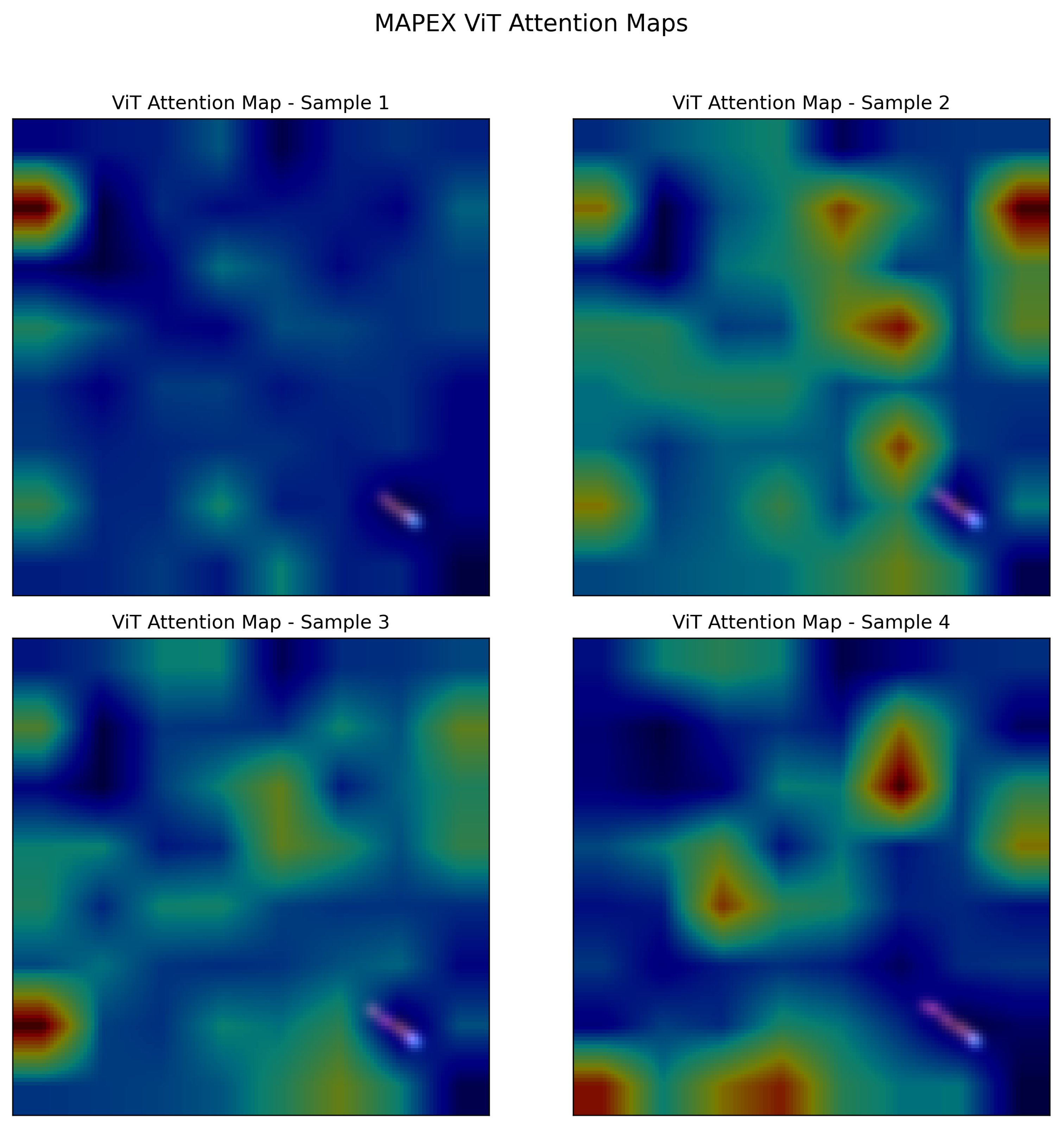
To examine what spatial patterns the visual encoder learns, we visualize the CLS token attention weights from the final Transformer block, reshaped to the  8 × 8  patch grid (Figure 5). Across diverse encounter geometries, the attention maps reveal consistent focus on trajectory intersection regions and vessel endpoints, which are precisely the areas most informative for predicting future motion and potential collision risk. Empty sea regions receive minimal attention, indicating that the model has learned selective spatial focus. This mirrors a human navigator’s tendency to focus on vessel proximity and convergence points, providing qualitative evidence that the visual representation enables meaningful spatial reasoning through data-driven training alone.

6.8. Prediction Horizon Analysis

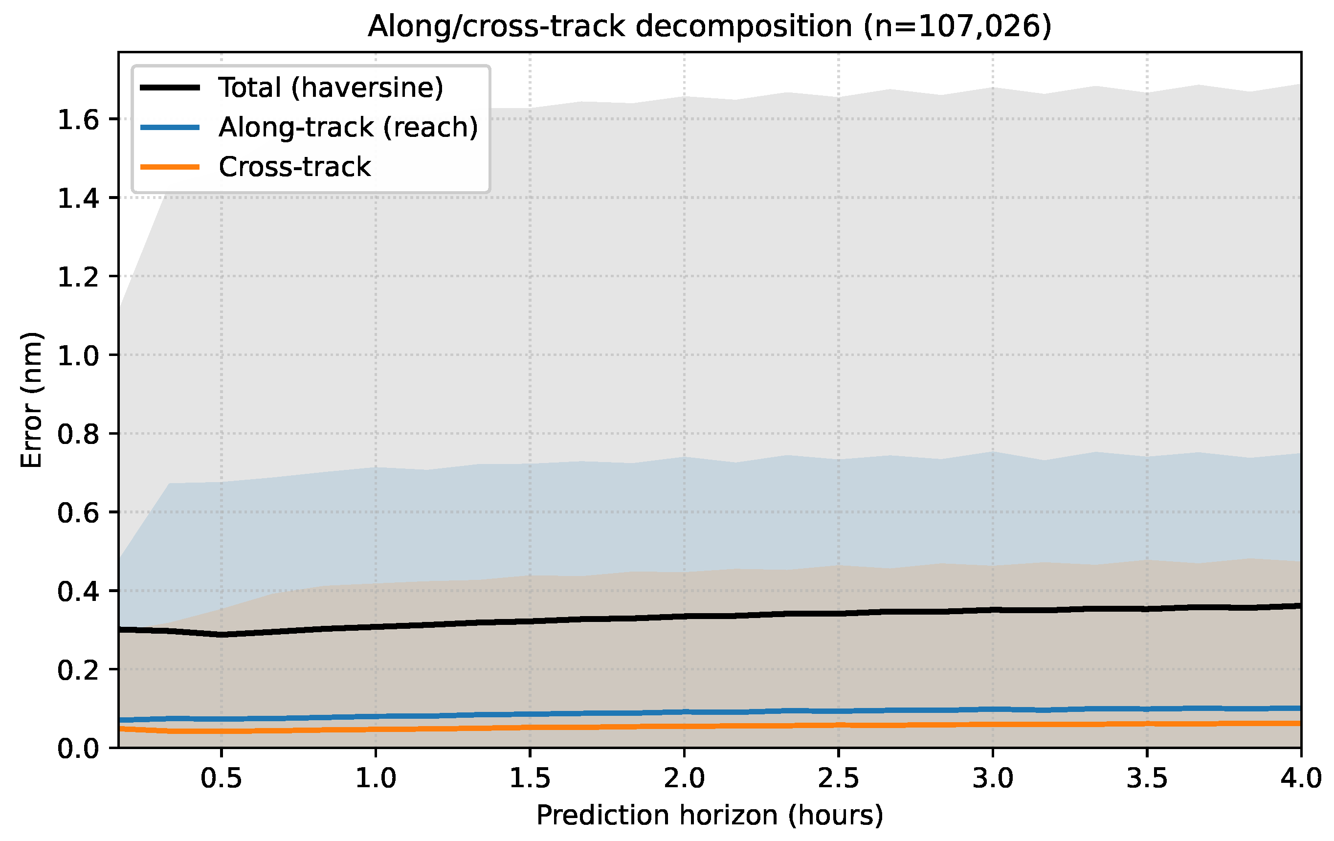
Figure 6 shows how prediction error evolves across the 24-step horizon, decomposed into along-track and cross-track components computed by projecting per-step displacement errors onto the unit direction of the ground-truth local velocity. ADE initially decreases during the first few steps as the GRU decoder benefits from strong short-term extrapolation from the last observed state, then grows steadily but remains moderate even at the 4-h mark. The gradual rather than exponential error growth suggests that the spatial scene context from the rasterized image constrains predictions to plausible regions throughout the forecast window, in contrast to purely autoregressive coordinate-domain models that tend to accumulate drift without such spatial anchoring. Along-track error dominates, consistent with the reach component being governed by along-path speed variation; cross-track error stays small, indicating that the model keeps the predicted trajectory close to the correct lane rather than drifting sideways. Overall means and per-sample standard deviations are summarized in Table 9.

6.8.1. Stratified Subsets: Speed, Scene Density, and Inter-Ship Distance

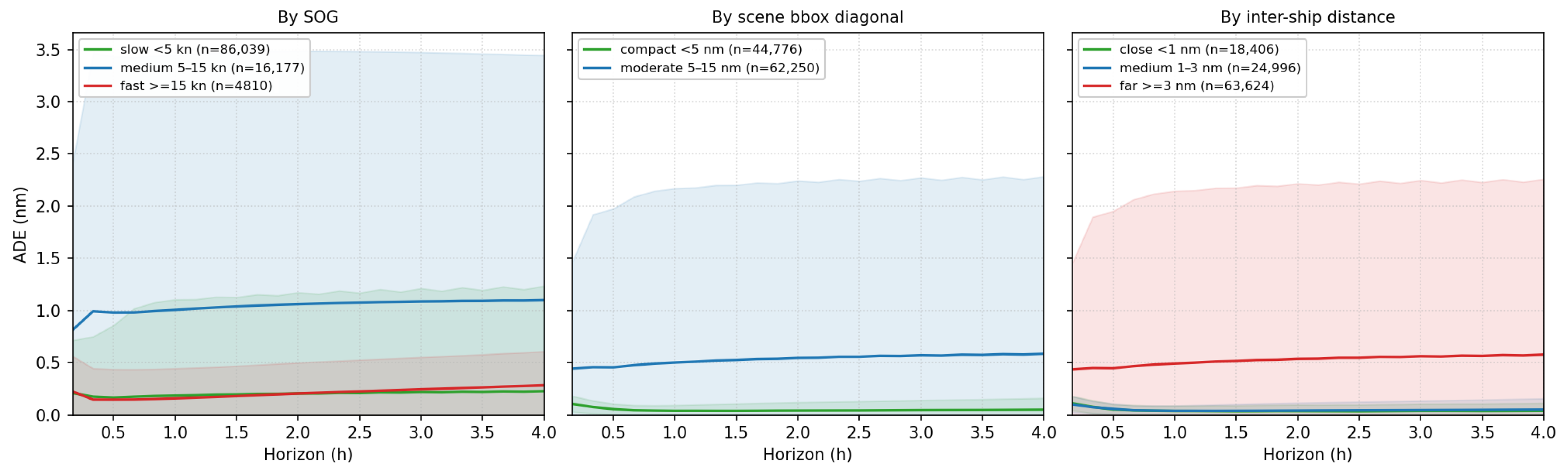
To diagnose whether the horizon-level averages conceal regime-dependent failure modes, we stratify the test samples by three covariates measured at the last observed time step: (i) speed over ground (SOG) of the predicted vessel, (ii) the diagonal of the shared scene bounding box as a proxy for scene density, and (iii) the inter-ship distance between the two vessels in the pair. Figure 7 plots per-step ADE with  ± 1  std bands for each bin, and Table 10 reports per-bin aggregate ADE and sample count. Ship-type stratification is not available because the Piraeus release does not publish ship-type codes; this is flagged as a limitation in Section 8.
The stratification exposes three readings. First, SOG shows a non-monotonic error profile: slow and fast vessels are both predicted accurately, while the medium-SOG bin is by far the hardest, several times worse than either extreme. We interpret this regime as capturing predominantly maneuvering vessels: port entry, departure, and harbor turns cluster in the 5–15 kn band, whereas slow-anchorage and open-water transit (the slow and fast bins, respectively) both follow near-straight-line motion that is substantially easier to extrapolate. This is a genuine limitation of Mapex—the model handles steady-state kinematics well but is less accurate on sharp course changes—and we report it explicitly rather than aggregating it into a single headline ADE. Second, inter-ship distance also shows a non-monotonic profile: close and medium pairs are predicted accurately while far pairs are noticeably harder. The far-pairs regime coincides with larger scene bounding boxes and therefore with coarser per-pixel resolution, which accounts for most of the residual error. The low close-passage ADE should be interpreted with care: close pairs in Piraeus are predominantly slow-moving, so the bin partly reflects a speed confound and cannot on its own separate “scene-geometry quality” from “slow-case easiness”; the directional conclusion that close passages are not blurred into far ones nonetheless follows, since the close bin is at least as accurate as the medium bin. Third, the wide-bbox bin is empty in the natural v2 MMSI-strict test distribution: wide-spread encounters simply do not occur with meaningful frequency in the Piraeus test month, which is the same dataset-level constraint that bounds the natural ambient-density range tested in Section 6.9.

6.8.2. Operational Metrics: CPA and COLREGs Encounter Classification

The per-channel ablation (Table 7) and the architectural ablation (Section 6.6) together identify a channel-specific division of labor between Mapex (full) and Mapex-V: the visual-only configuration achieves lower position error (lat/lon/SOG), while the full configuration achieves better course-over-ground accuracy. To translate this finding from per-channel MSE into operationally interpretable metrics, we evaluate both configurations on two derived quantities computed from their predicted trajectories on the Piraeus v1 test set.
Closest Point of Approach (CPA) error is the absolute difference between predicted and ground-truth minimum inter-ship distance over the 24-step horizon, computed per encounter. CPA depends only on lat/lon trajectories and is therefore expected to favor whichever model is more accurate on position channels.
COLREGs encounter classification accuracy is computed at the predicted time of CPA (TCPA): given the predicted COGs of both ships and the predicted bearing between them, we classify the encounter as head-on, crossing, overtake-ship-i-overtaking, or overtake-ship-j-overtaking, following standard COLREGs Rules 13–15 thresholds. We report classification accuracy against the corresponding labels computed from the ground-truth trajectories. Because this metric is determined by the relative orientation of vessel tracks rather than by raw position, it is sensitive to COG accuracy specifically.
Table 11 reports both metrics on all  N = 402 , 733  pairwise encounters in the Piraeus v1 test set and on the operationally-relevant subset of close encounters (ground-truth CPA  < 1  nm,  n = 75 , 994 ).
The two metric families partition cleanly along their input dependence. Mapex-V achieves the lower CPA error in both regimes, with the gap widening on the close-encounter subset, consistent with its position-channel advantage. Mapex (full) achieves the higher COLREGs classification accuracy in both regimes, with the gap most pronounced on the close-encounter subset, where COLREGs maneuver decisions are made and the encounter-type classification determines whether a port-to-port pass, a starboard-to-starboard pass, or an overtaking maneuver is the appropriate response. The accuracy gap on this operationally critical subset therefore reflects a measurable operational benefit of retaining the coordinate branch, not merely a per-channel MSE artifact. Section 7 returns to this trade-off and to its implications for the choice of Mapex (full) as the primary configuration.

6.9. Scalability Across Vessel Counts

The pairwise main experiments evaluate Mapex on encounters of two vessels at a time, but Piraeus traffic naturally includes scenes in which more than two vessels are within proximity at the encounter time. To support the scalability argument advanced in Section 7.3 and to address Reviewer 3’s concern that scalability claims cannot be supported by an 8-vessel experimental range alone, we evaluate the existing pairwise Mapex (5-seed full, seed 42 checkpoint) under varying ambient density: for each test pair we record the size N of the surrounding scene (the number of vessels in proximity at the encounter time, recovered by re-running the scene-detection BFS on the test month with a generous size cap). We then aggregate ADE/FDE per scene size. Table 12 reports the result.
Two readings follow. First, accuracy does not degrade as ambient density increases over the natural Piraeus range; if anything, ADE and FDE drift slightly lower at  N = 3  and  N = 4 . We do not attribute this to the architecture being intrinsically better at higher N: denser scenes coincide with the same slow-vessel regime that drove the close-passage low-ADE bin in Section 6.8.1 (port-approach traffic moves slowly and follows tight, recurring routes), so the apparent improvement carries a speed confound and should be read as “the architecture does not collapse at higher ambient density” rather than “denser is genuinely easier”. Second,  N > 4  is not represented in the natural Piraeus test month: this is a corpus property, not a model limitation, and validating the scalability argument at higher densities therefore requires a denser-traffic corpus (e.g., a major container port) and is left as future work. The architectural-complexity claim itself—that the rasterization paradigm scales linearly in vessel count by construction (each additional vessel adds three input channels but does not increase the ViT token count or attention complexity)—holds independently of whether  N > 4  scenes are tested.

6.10. Cross-Port Generalization

The Piraeus experiments establish Mapex’s accuracy on a single port. To assess whether the architecture and visual representation transfer to qualitatively different traffic regimes rather than overfitting to Piraeus-specific recurring ferry routes, we retrain Mapex from scratch on two NOAA MarineCadastre 2022 corpora: Los Angeles/Long Beach (LA, January–February 2022, 59 days,  33.55 33 . 85  N/ 118.35 118 . 00  E), a Pacific container hub dominated by long approach transits, and San Francisco Bay (SF, January 2022, 31 days), a mixed Bay–ferry/container regime. Both ports use an MMSI-strict split in which train and test vessels are disjoint by construction, so the evaluation does not benefit from the recurring-vessel statistics that characterize Piraeus. Hyperparameters are kept identical to the Piraeus configuration, and we apples-to-apples re-train the reference TrAISformer baseline on the same MMSI-strict splits at each port. Table 13 reports the result.
Three readings follow. First, the Mapex architecture, retrained from scratch on two US ports with different traffic regimes and under MMSI-strict evaluation, produces sub-nautical-mile predictions in both cases, ruling out the reading that the spatial-visual representation is locked to the Piraeus corpus. Second, in head-to-head retraining under identical MMSI-strict protocols, Mapex outperforms TrAISformer by roughly an order of magnitude at both ports; we note that TrAISformer’s ∼57 M-parameter autoregressive architecture overfits quickly on the order of  10 4  trajectories available at these ports (its validation loss stops improving after epoch 2), so these numbers reflect the reference implementation at this data scale rather than its published best, and the comparison should be read as “under equal training budget on this corpus”. Third, the relative ordering of Mapex (full) and Mapex-V is not consistent across corpora: on LA (∼11 K train samples) Mapex-V is modestly better, on SF (∼16 K) Mapex (full) is better, and on Piraeus v1 (∼217 K) the two are within seed variance. This pattern is consistent with the coordinate branch needing a sufficiently large training pool to disambiguate signal from noise; we report both variants transparently per port rather than selecting the more favorable one. A broader multi-port study with more diverse training corpora and ship-type stratification is left for future work (Section 7.3).

6.11. Qualitative Analysis

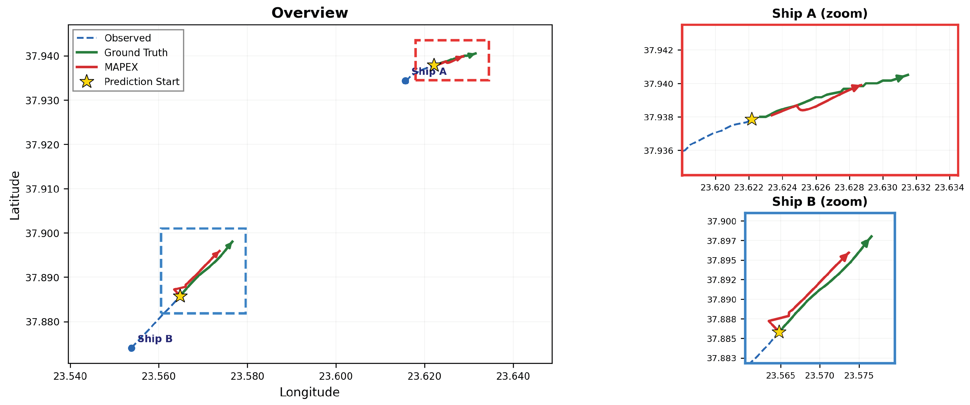
Figure 8 presents representative prediction examples from the Piraeus test set. The selected samples illustrate encounters where both vessels are actively maneuvering, providing a meaningful test of the model’s ability to capture dynamic interaction patterns.
In the example shown, two vessels navigate through the Saronic Gulf with Ship A in the upper region heading northeast and Ship B in the lower-left region also moving northeast, separated by approximately 4–5 nm. Despite the spatial separation, the shared rasterized image encodes both vessels’ trajectories as visible spatial patterns, enabling the model to predict both simultaneously. Mapex predictions closely track the ground truth for both vessels: Ship A’s northeastward progression with a slight course adjustment is captured accurately, and Ship B’s trajectory is also reproduced with high fidelity.
These results illustrate the advantage of spatial visualization over coordinate processing: because both vessels’ movements are encoded as visual features in a shared image, the model naturally produces spatially coherent predictions without physically implausible jumps or discontinuities. The zoomed views confirm that sub-nautical-mile-level accuracy is maintained throughout the 4-h prediction horizon, consistent with the quantitative results in Table 3.

7. Discussion

7.1. Spatial Visualization vs. Coordinate Processing

The core insight behind Mapex is that how information is represented matters as much as how it is processed. Coordinate-domain models receive vessel states as sequences of numerical tuples  ( lat , lon , SOG , COG , heading )  and must infer spatial relationships such as relative positions, convergence angles, and closing speeds through learned arithmetic over these numbers. This places a significant burden on the model: multi-vessel interaction patterns must be extracted from interleaved or separately encoded number sequences without any explicit spatial structure.
Mapex takes a fundamentally different approach by converting these same coordinates into a spatial visual representation. In the rasterized image, the information that coordinate models must laboriously compute becomes directly observable: converging trajectories appear as lines approaching each other, speed differentials manifest as differences in track density and brightness, headings are visible as trajectory curvature, and the overall spatial layout of an encounter is immediately apparent. This visual representation provides the same information as coordinate sequences but organized spatially rather than sequentially, enabling a visual encoder to leverage spatial inductive biases that coordinate-domain models lack.
The experimental results support this interpretation. Mapex substantially outperforms coordinate-domain Transformer baselines despite using a simpler architecture and pure MSE loss, suggesting that the richer spatial representation, rather than model sophistication, drives the performance gap. The attention visualization (Figure 5) further confirms that the visual encoder focuses on spatially meaningful regions (trajectory intersections, vessel endpoints), a behavior that emerges naturally from the visual representation without explicit supervision.
The coordinate branch in Mapex is best understood as an architectural component that carries the course-over-ground information the raster cannot express, rather than as a redundancy with the visual branch. Although the rasterized image is derived from the raw coordinates, the rasterization is not lossless: it carries lat/lon, SOG, and heading as explicit channels but does not raster course-over-ground, which differs from heading under drift and current. A model that consumed only the raster would therefore be structurally unable to satisfy the five-channel output specification Mapex commits to. The 5-seed ablation in Table 6 together with the per-channel breakdown in Table 7 confirms this division-of-labor reading empirically, as an observed outcome rather than a causally proven one. On position metrics (ADE/FDE, which use only lat/lon), Mapex-V (visual-only) outperforms the full model and Mapex-C (coord-only) essentially matches it; the visual encoder alone is sufficient for position prediction at sub-nautical-mile accuracy. On per-channel MSE, however, the coordinate branch reduces error specifically on course-over-ground while leaving lat, lon, SOG, and heading either no better or slightly worse; we read this pattern as the branch functioning as a channel-specific pathway rather than as a general position-accuracy enhancement.
This produces a channel-by-channel trade-off between two reportable configurations rather than an unambiguous winner. Mapex-V minimizes position error (lat/lon/SOG) and is the natural choice for applications that need only position tracking. Mapex (full) accepts slightly higher position error in exchange for substantially better COG accuracy, with heading essentially tied between the two. The operational metrics in Section 6.8.2 confirm that this trade-off is empirically meaningful and not just a per-channel MSE artifact: Mapex-V wins on CPA accuracy as expected from its position advantage, while Mapex (full) wins on COLREGs encounter-type classification—the regime-discriminating metric that determines which maneuver rule applies—with the margin concentrated on the close-encounter subset where such decisions are actually made. We therefore report Mapex (full) as the primary configuration, consistent with the paper’s specification of a complete five-channel kinematic forecaster (Section 4.4) and now empirically supported by the COLREGs operational metric, and we report Mapex-V transparently as a position-focused alternative rather than treating it as an oversight or deficiency to be hidden. A full closed-loop simulator validation that evaluates downstream maneuver execution remains future work.

7.2. Physical Movement as Visual Pattern

A distinctive strength of the rasterization approach is how it makes physical movement characteristics visually accessible. In coordinate sequences, a vessel’s kinematic state is encoded as abstract numbers: SOG as a scalar, heading as an angle. Recognizing patterns like “vessel A is decelerating while vessel B maintains speed” requires the model to track numerical changes across timesteps.
In the rasterized image, the same kinematic information appears as visual texture. The trajectory heatmap’s temporal gradient encodes motion history so that recent positions appear brighter, making direction and acceleration patterns visible at a glance. The speed field channel renders velocity as pixel intensity along the track, so fast-moving and slow-moving vessels are visually distinct. The heading field encodes directional state as a color gradient, making turns and course changes spatially apparent. These visual encodings transform what would be abstract numerical patterns into spatial textures that a visual encoder can process with the same mechanisms used for natural image understanding.
This paradigm is encoder-agnostic: while we adopt a Vision Transformer for its effective global attention across image patches, the core contribution lies in the rasterization representation itself. Any visual encoder capable of spatial reasoning, whether convolutional networks, Swin Transformers, or future architectures, could process these trajectory images, as the spatial structure is an inherent property of the representation, not the encoder.

7.3. Scalability and Limitations

Architecturally, the rasterization paradigm scales linearly in vessel count: adding a vessel simply adds three channels to the input image, and the visual encoder processes all vessels simultaneously without any change in network topology. In contrast, coordinate-domain approaches face quadratic scaling, as pairwise models must process all  N 2  vessel pairs and graph-based approaches [12] must maintain edge representations for each pair. Empirically (Section 6.9, Table 12), accuracy on Piraeus pairs does not degrade as ambient scene density grows over the natural range  N { 2 , 3 , 4 } . The Piraeus corpus is sparse, so  N > 4  scenes do not occur with meaningful frequency; validating the scalability argument at denser regimes (e.g., large-port approaches with  N 10 ) requires a denser-traffic corpus and is left as future work. The architectural property remains: at any N, cost scales linearly in channel count rather than quadratically in pair count.
However, the fixed image resolution introduces a precision ceiling. For encounters spanning several nautical miles, each pixel represents tens of meters, which suffices for route-level prediction but may limit close-quarters maneuvering accuracy. The coordinate branch partially mitigates this quantization, and differentiable rendering or multi-resolution strategies could further close the gap in future work. The trajectory-to-image conversion also introduces data pipeline overhead, though this cost is incurred once per sample and is amenable to caching. Cross-port retraining on Los Angeles and San Francisco (Section 6.10) shows that the architecture and representation transfer to qualitatively different traffic regimes when local statistics are refit, although a checkpoint trained on one port is not expected to deploy zero-shot to another whose coordinate distribution differs; a broader multi-port study is part of the future work outlined below.

8. Conclusions

We presented Mapex, a vision-based framework that reframes ship trajectory prediction as a spatial understanding task. By rasterizing multi-vessel AIS trajectories into chart-like multi-channel images, Mapex converts coordinate sequences into spatial visual representations where physical movement patterns such as trajectory shapes, speed differentials, and heading changes become directly observable features rather than abstract numerical values. A parallel coordinate branch supplies the course-over-ground information that the raster does not encode explicitly, supporting the complete five-channel kinematic output that operational use cases require; this is an architectural choice reflecting the paper’s target use rather than a claim of empirical dominance over the visual-only variant on position metrics (see Section 7).
Experiments on the Piraeus AIS dataset demonstrate that Mapex outperforms all coordinate-domain Transformer baselines and recent LLM-based approaches by a substantial margin, suggesting that the spatial visual representation, rather than model complexity, is the key driver of prediction accuracy. The rasterization approach is encoder-agnostic, scales linearly in channel count with the number of vessels by construction, and offers domain agnosticism that enables potential transfer to other multi-agent prediction domains. Empirically, accuracy on Piraeus pairs does not degrade as ambient scene density grows over the natural range  N { 2 , 3 , 4 }  (Section 6.9); validating the architectural scalability at higher densities requires a denser-traffic corpus and is part of the future work below.
Future work will explore higher-resolution rasterization with differentiable rendering, alternative visual encoder architectures to further validate the representation-centric contribution, cross-domain evaluation on the DMA AIS dataset,  ( sin , cos )  encoding of the angular channels (COG, heading) to remove the residual  0 / 360  wraparound penalty documented in the per-channel MSE breakdown, a systematic study of location-specificity across ports with larger training corpora than the LA/SF pilot reported in Section 6.10, and closed-loop validation of the position-vs-COG configuration choice (Section 7.1) in a collision-avoidance simulator—the reported ADE/FDE are open-loop forecasting accuracy and do not directly measure operational safety margins.

Author Contributions

Conceptualization, J.B.; methodology, J.B.; software, J.B.; validation, J.B.; formal analysis, J.B.; investigation, J.B.; resources, J.B. and K.-Y.L.; data curation, J.B.; writing—original draft preparation, J.B.; writing—review and editing, K.-Y.L.; visualization, J.B.; supervision, K.-Y.L.; project administration, K.-Y.L. All authors have read and agreed to the published version of the manuscript.

Funding

This work was supported by the Hankuk University of Foreign Studies Research Fund of 2026.

Data Availability Statement

The Piraeus AIS dataset analyzed in this study is publicly available on Zenodo at https://zenodo.org/records/6323416 (DOI: https://doi.org/10.1016/j.dib.2021.107782) (accessed on 6 May 2026), as released by Tritsarolis et al. [42]. No new primary data were generated in this study.

Conflicts of Interest

The authors declare no conflicts of interest.

References

  1. Zhong, Y.; Zhou, H.; Grifoll, M.; Martín, A.; Zhou, Y.; Liu, J.; Zheng, P. A Novel Method for Holistic Collision Risk Assessment in the Precautionary Area Using AIS Data. Systems 2025, 13, 338. [Google Scholar] [CrossRef]
  2. Zhao, Z.; Liu, X.; Feng, L.; Grifoll, M.; Feng, H. Causation Analysis of Marine Traffic Accidents Using Deep Learning Approaches: A Case Study from China’s Coasts. Systems 2025, 13, 284. [Google Scholar] [CrossRef]
  3. Gao, M.; Shi, G.; Li, S. Online Prediction of Ship Behavior with Automatic Identification System Sensor Data Using Bidirectional Long Short-Term Memory Recurrent Neural Network. Sensors 2018, 18, 4211. [Google Scholar] [CrossRef] [PubMed]
  4. Park, J.; Jeong, J.; Park, Y. Ship Trajectory Prediction Based on Bi-LSTM Using Spectral-Clustered AIS Data. J. Mar. Sci. Eng. 2021, 9, 1037. [Google Scholar] [CrossRef]
  5. Nguyen, D.; Fablet, R. TrAISformer: A Transformer Network with Sparse Augmented Data Representation and Cross Entropy Loss for AIS-Based Vessel Trajectory Prediction. IEEE Access 2024, 12, 21596–21609. [Google Scholar] [CrossRef]
  6. Liu, Y.; Hu, T.; Zhang, H.; Wu, H.; Wang, S.; Ma, L.; Long, M. iTransformer: Inverted Transformers Are Effective for Time Series Forecasting. In Proceedings of the International Conference on Learning Representations (ICLR), Vienna, Austria, 7–11 May 2024. [Google Scholar]
  7. Park, H.; Jung, J.; Seo, M.; Choi, H.; Cho, D.; Park, S.; Choi, D.G. AIS-LLM: A Unified Framework for Maritime Trajectory Prediction, Anomaly Detection, and Collision Risk Assessment with Explainable Forecasting. arXiv 2025, arXiv:2508.07668. [Google Scholar] [CrossRef]
  8. International Maritime Organization. Convention on the International Regulations for Preventing Collisions at Sea, 1972 (COLREGs), as Amended; IMO Publishing: London, UK, 1972; Available online: https://www.imo.org/en/About/Conventions/Pages/COLREG.aspx (accessed on 6 May 2026).
  9. Murray, B.; Perera, L.P. An AIS-Based Deep Learning Framework for Regional Ship Behavior Prediction. Reliab. Eng. Syst. Saf. 2021, 215, 107819. [Google Scholar] [CrossRef]
  10. Li, H.; Jiao, H.; Yang, Z. AIS Data-Driven Ship Trajectory Prediction Modelling and Analysis Based on Machine Learning and Deep Learning Methods. Transp. Res. Part E Logist. Transp. Rev. 2023, 175, 103152. [Google Scholar] [CrossRef]
  11. Zhang, X.; Fu, X.; Xiao, Z.; Xu, H.; Qin, Z. Vessel Trajectory Prediction in Maritime Transportation: Current Approaches and Beyond. IEEE Trans. Intell. Transp. Syst. 2022, 23, 19980–19998. [Google Scholar] [CrossRef]
  12. Zhang, X.; Liu, J.; Gong, P.; Chen, C.; Han, B.; Wu, Z. Trajectory Prediction of Seagoing Ships in Dynamic Traffic Scenes via a Gated Spatio-Temporal Graph Aggregation Network. Ocean Eng. 2023, 287, 115886. [Google Scholar] [CrossRef]
  13. Vaswani, A.; Shazeer, N.; Parmar, N.; Uszkoreit, J.; Jones, L.; Gomez, A.N.; Kaiser, Ł.; Polosukhin, I. Attention Is All You Need. In Proceedings of the 31st Conference on Neural Information Processing Systems (NeurIPS 2017), Long Beach, CA, USA, 4–9 December 2017; Volume 30, pp. 5998–6008. [Google Scholar]
  14. Dosovitskiy, A.; Beyer, L.; Kolesnikov, A.; Weissenborn, D.; Zhai, X.; Unterthiner, T.; Dehghani, M.; Minderer, M.; Heigold, G.; Gelly, S.; et al. An Image is Worth 16x16 Words: Transformers for Image Recognition at Scale. In Proceedings of the International Conference on Learning Representations (ICLR), Vienna, Austria, 3–7 May 2021. [Google Scholar]
  15. Touvron, H.; Cord, M.; Douze, M.; Massa, F.; Sablayrolles, A.; Jégou, H. Training Data-Efficient Image Transformers & Distillation Through Attention. In Proceedings of the International Conference on Machine Learning, Vienna, Austria, 18–24 July 2021; pp. 10347–10357. [Google Scholar]
  16. Liu, Z.; Lin, Y.; Cao, Y.; Hu, H.; Wei, Y.; Zhang, Z.; Lin, S.; Guo, B. Swin Transformer: Hierarchical Vision Transformer Using Shifted Windows. In Proceedings of the IEEE/CVF International Conference on Computer Vision, Montreal, BC, Canada, 11–17 October 2021; pp. 10012–10022. [Google Scholar]
  17. Bao, H.; Dong, L.; Piao, S.; Wei, F. BEiT: BERT Pre-Training of Image Transformers. In Proceedings of the International Conference on Learning Representations (ICLR), Virtual, 25–29 April 2022. [Google Scholar]
  18. Riquelme, C.; Puigcerver, J.; Mustafa, B.; Neumann, M.; Jenatton, R.; Pinto, A.S.; Keysers, D.; Houlsby, N. Scaling Vision with Sparse Mixture of Experts. In Proceedings of the 35th Conference on Neural Information Processing Systems (NeurIPS 2021), Online, 6–14 December 2021; Volume 34, pp. 8583–8595. [Google Scholar]
  19. Cheng, R.; An, X.; Xu, Y. Vit-Traj: A Spatial–Temporal Coupling Vehicle Trajectory Prediction Model Based on Vision Transformer. Systems 2025, 13, 147. [Google Scholar] [CrossRef]
  20. Helbing, D.; Molnár, P. Social Force Model for Pedestrian Dynamics. Phys. Rev. E 1995, 51, 4282–4286. [Google Scholar] [CrossRef]
  21. Alahi, A.; Goel, K.; Ramanathan, V.; Robicquet, A.; Fei-Fei, L.; Savarese, S. Social LSTM: Human Trajectory Prediction in Crowded Spaces. In Proceedings of the IEEE Conference on Computer Vision and Pattern Recognition (CVPR), Las Vegas, NV, USA, 27–30 June 2016; pp. 961–971. [Google Scholar]
  22. Mohamed, A.; Qian, K.; Elhoseiny, M.; Claudel, C. Social-STGCNN: A Social Spatio-Temporal Graph Convolutional Neural Network for Human Trajectory Prediction. In Proceedings of the IEEE/CVF Conference on Computer Vision and Pattern Recognition (CVPR), Seattle, WA, USA, 14–19 June 2020; pp. 14424–14432. [Google Scholar]
  23. Sadeghian, A.; Kosaraju, V.; Sadeghian, A.; Hirose, N.; Rezatofighi, H.; Savarese, S. SoPhie: An Attentive GAN for Predicting Paths Compliant to Social and Physical Constraints. In Proceedings of the IEEE/CVF Conference on Computer Vision and Pattern Recognition (CVPR), Honolulu, HI, USA, 21–26 July 2019; pp. 1349–1358. [Google Scholar]
  24. Salzmann, T.; Ivanovic, B.; Chakravarty, P.; Pavone, M. Trajectron++: Dynamically-Feasible Trajectory Forecasting with Heterogeneous Data. In Proceedings of the European Conference on Computer Vision (ECCV), Glasgow, UK, 23–28 August 2020; pp. 683–700. [Google Scholar]
  25. Mangalam, K.; Girase, H.; Agarwal, S.; Lee, K.H.; Adeli, E.; Malik, J.; Gaidon, A. It Is Not the Journey but the Destination: Endpoint Conditioned Trajectory Prediction. In Proceedings of the European Conference on Computer Vision (ECCV), Glasgow, UK, 23–28 August 2020; pp. 759–776. [Google Scholar]
  26. Yuan, Y.; Weng, X.; Ou, Y.; Kitani, K.M. AgentFormer: Agent-Aware Transformers for Socio-Temporal Multi-Agent Forecasting. In Proceedings of the 2021 IEEE/CVF International Conference on Computer Vision (ICCV), Montreal, BC, Canada, 11–17 October 2021; pp. 9813–9823. [Google Scholar]
  27. Xu, C.; Tan, R.T.; Tan, Y.; Chen, S.; Wang, Y.; Wang, X.; Wang, Y. EqMotion: Equivariant Multi-Agent Motion Prediction with Invariant Interaction Reasoning. In Proceedings of the IEEE/CVF Conference on Computer Vision and Pattern Recognition (CVPR), Vancouver, BC, Canada, 17–24 June 2023; pp. 1410–1420. [Google Scholar]
  28. Bansal, M.; Krizhevsky, A.; Ogale, A. ChauffeurNet: Learning to Drive by Imitating the Best and Synthesizing the Worst. In Proceedings of the Robotics: Science and Systems (RSS), Breisgau, Germany, 22–26 June 2019. [Google Scholar]
  29. Cui, H.; Radosavljevic, V.; Chou, F.C.; Lin, T.H.; Nguyen, T.; Huang, T.K.; Schneider, J.; Djuric, N. Multimodal Trajectory Predictions for Autonomous Driving Using Deep Convolutional Networks. In Proceedings of the IEEE International Conference on Robotics and Automation (ICRA), Montreal, QC, Canada, 20–24 May 2019; pp. 2090–2096. [Google Scholar]
  30. Phan-Minh, T.; Grigore, E.C.; Boulton, F.A.; Beijbom, O.; Wolff, E.M. CoverNet: Multimodal Behavior Prediction Using Trajectory Sets. In Proceedings of the 2020 IEEE/CVF Conference on Computer Vision and Pattern Recognition (CVPR), Seattle, WA, USA, 14–19 June 2020; pp. 14062–14071. [Google Scholar]
  31. Djuric, N.; Radosavljevic, V.; Cui, H.; Nguyen, T.; Chou, F.C.; Lin, T.H.; Singh, N.; Schneider, J. Uncertainty-Aware Short-Term Motion Prediction of Traffic Actors for Autonomous Driving. In Proceedings of the IEEE Winter Conference on Applications of Computer Vision (WACV), Snowmass Village, CO, USA, 1–5 March 2020; pp. 2084–2093. [Google Scholar]
  32. Li, Z.; Wang, W.; Li, H.; Xie, E.; Sima, C.; Lu, T.; Yu, Q.; Dai, J. BEVFormer: Learning Bird’s-Eye-View Representation from Multi-Camera Images via Spatiotemporal Transformers. In Proceedings of the European Conference on Computer Vision (ECCV), Tel Aviv, Israel, 23–27 October 2022; pp. 1–18. [Google Scholar]
  33. Philion, J.; Fidler, S. Lift, Splat, Shoot: Encoding Images from Arbitrary Camera Rigs by Implicitly Unprojecting to 3D. In Proceedings of the European Conference on Computer Vision (ECCV), Glasgow, UK, 23–28 August 2020; pp. 194–210. [Google Scholar]
  34. Lang, A.H.; Vora, S.; Caesar, H.; Zhou, L.; Yang, J.; Beijbom, O. PointPillars: Fast Encoders for Object Detection from Point Clouds. In Proceedings of the IEEE/CVF Conference on Computer Vision and Pattern Recognition (CVPR), Long Beach, CA, USA, 16–20 June 2019; pp. 12697–12705. [Google Scholar]
  35. Yin, T.; Zhou, X.; Krähenbühl, P. Center-Based 3D Object Detection and Tracking. In Proceedings of the IEEE/CVF Conference on Computer Vision and Pattern Recognition (CVPR), Nashville, TN, USA, 20–25 June 2021; pp. 11784–11793. [Google Scholar]
  36. Ngiam, J.; Caine, B.; Vasudevan, V.; Zhang, Z.; Chiang, H.T.L.; Ling, J.; Roelofs, R.; Bewley, A.; Liu, C.; Venugopal, A.; et al. Scene Transformer: A Unified Architecture for Predicting Multiple Agent Trajectories. In Proceedings of the International Conference on Learning Representations (ICLR), Virtual, 25–29 April 2022. [Google Scholar]
  37. Xu, L.; Chen, N.; Chen, Z.; Zhang, C.; Yu, H. Spatiotemporal Forecasting in Earth System Science: Methods, Uncertainties, Predictability and Future Directions. Earth-Sci. Rev. 2021, 222, 103828. [Google Scholar] [CrossRef]
  38. Xu, L.; Chen, N.; Yang, C.; Yu, H.; Chen, Z. Quantifying the Uncertainty of Precipitation Forecasting Using Probabilistic Deep Learning. Hydrol. Earth Syst. Sci. 2022, 26, 2923–2938. [Google Scholar] [CrossRef]
  39. Yu, H.; Jiang, C.; Fang, Q.; Wei, T.; Xu, L. Deep Learning Driven Spatiotemporal Prediction of Global Carbon Emissions from Container Shipping. Transp. Res. Part D Transp. Environ. 2026, 151, 105169. [Google Scholar] [CrossRef]
  40. Yu, H.; Cui, X.; Bai, X.; Chen, C.; Xu, L. Incorporating Graph Theory and Time Series Analysis for Fine-Grained Traffic Flow Prediction in Port Areas. Ocean Eng. 2025, 335, 121693. [Google Scholar] [CrossRef]
  41. Cho, K.; van Merriënboer, B.; Gulcehre, C.; Bahdanau, D.; Bougares, F.; Schwenk, H.; Bengio, Y. Learning Phrase Representations Using RNN Encoder–Decoder for Statistical Machine Translation. In Proceedings of the the 2014 Conference on Empirical Methods in Natural Language Processing (EMNLP), Doha, Qatar, 25–29 October 2014; pp. 1724–1734. [Google Scholar]
  42. Tritsarolis, A.; Kontoulis, Y.; Theodoridis, Y. The Piraeus AIS Dataset for Large-Scale Maritime Data Analytics. Data Brief 2022, 40, 107782. [Google Scholar] [CrossRef] [PubMed]
  43. Zhao, L.; Shi, G.; Yang, J. An Adaptive Hierarchical Clustering Method for Ship Trajectory Data Based on DBSCAN Algorithm. In Proceedings of the IEEE 2nd International Conference on Big Data Analysis (ICBDA), Beijing, China, 10–12 March 2017; pp. 329–336. [Google Scholar]
  44. Guo, S.; Mou, J.; Chen, L.; Chen, P. Improved Kinematic Interpolation for AIS Trajectory Reconstruction. Ocean Eng. 2021, 234, 109258. [Google Scholar] [CrossRef]
  45. Kontopoulos, I.; Varlamis, I.; Tserpes, K. A Distributed Framework for Extracting Maritime Traffic Patterns. Int. J. Geogr. Inf. Sci. 2021, 35, 767–792. [Google Scholar] [CrossRef]
  46. Zhou, H.; Zhang, S.; Peng, J.; Zhang, S.; Li, J.; Xiong, H.; Zhang, W. Informer: Beyond Efficient Transformer for Long Sequence Time-Series Forecasting. In Proceedings of the Thirty-Fifth AAAI Conference on Artificial Intelligence, Vancouver, BC, Canada, 2–9 February 2021; Volume 35, pp. 11106–11115. [Google Scholar]
Figure 1. Overview of the Mapex framework. Raw AIS coordinate sequences for all vessels are co-registered onto a single shared  128 × 128  canvas defined by one common adaptive bounding box, and each vessel contributes its own three channels (trajectory heatmap, speed field, heading field) on that shared canvas, yielding a  3 N -channel scene tensor; the per-vessel decomposition is along the channel axis, so the multiple trajectories visible in the localization panel correspond to per-vessel channels rendered on the same coordinate frame rather than to a single mixed-channel image. A visual encoder extracts a global scene representation, which is fused with per-ship coordinate embeddings from a parallel numeric branch. The fused representation feeds an autoregressive GRU decoder that predicts future trajectories for all vessels. Per-vessel channels are rendered with vessel-specific hues.
Systems 14 00536 g001
Figure 2. Detailed architecture of Mapex. Left: the rasterization pipeline converts N vessels’ coordinate sequences into a  3 N -channel spatial image. Center: a visual encoder (ViT with 6 blocks, 8 heads,  d = 256 ) processes 64 patches from the  128 × 128  image, producing a CLS token as global scene representation. A parallel coordinate branch (MLP,  90 128 128 ) preserves per-ship numeric precision. Right: the fusion MLP combines both streams, and an autoregressive GRU decoder generates 24-step predictions for each vessel.
Systems 14 00536 g002
Figure 3. Trajectory rasterization pipeline. Raw AIS coordinates for multiple vessels are mapped to a  128 × 128  canvas with an adaptive bounding box (20% margin). Each vessel produces three channels: trajectory heatmap with temporal gradient (brighter = more recent), speed field, and heading field. The resulting multi-channel image captures the complete observable state of the multi-vessel encounter as a spatial visual representation.
Systems 14 00536 g003
Figure 4. End-to-end Mapex on a representative pairwise encounter from the Piraeus test set. Six left panels: actual rendered input channels for both vessels (Ship A row, Ship B row); columns show the trajectory heatmap (temporal gradient: brighter = more recent), the speed field, and the heading field. Right panel: scene overlay with observed history (blue), ground-truth future (green), and Mapex prediction (red) on the adaptive bounding-box coordinate frame. The heatmap panels are rendered on the fixed  128 × 128  square canvas that the model actually consumes; because the adaptive bounding box is generally non-square in degrees, the apparent slope of a track on the canvas differs from its geographic slope in the scene overlay by the bounding-box aspect ratio. The chosen sample contains a non-trivial maneuver to make the model behavior visible, so the individual ADE is naturally above the dataset-wide 5-seed mean of  0.153  nm.
Systems 14 00536 g004
Figure 5. CLS token attention maps from the final ViT Transformer block across four encounter samples. Warmer colors indicate higher attention weights. The model consistently attends to trajectory intersection regions and vessel endpoints.
Systems 14 00536 g005
Figure 6. Per-step prediction error over the 24-step horizon (4 h at 10-min intervals) decomposed into along-track (reach, parallel to ground-truth velocity) and cross-track (perpendicular) components, with  ± 1  std bands. Evaluated on the v2 MMSI-strict test split ( n = 107 , 026  predicted trajectories, seed 42). The total haversine error grows gradually rather than exponentially, and the decomposition shows that along-track error dominates throughout the horizon, with cross-track error staying small and nearly flat.
Systems 14 00536 g006
Figure 7. Per-step ADE over the 4-h horizon stratified by (left) speed over ground, (middle) scene bbox diagonal, and (right) inter-ship distance, with  ± 1  std bands. Bins with zero samples (e.g., wide scenes  15  nm in the Piraeus test split) are omitted. Close-passage pairs (<1 nm,  n = 18 , 406 ) are not systematically harder than medium-distance pairs, confirming that the shared-canvas representation does not blur close from far encounters.
Systems 14 00536 g007
Figure 8. Qualitative prediction results on a pairwise encounter from the Piraeus AIS test set. Left: overview showing the full spatial context with observed trajectories (blue dashed), ground truth future positions (green), and Mapex predictions (red). Right: zoomed views of each vessel’s prediction region. The spatial visualization enables the model to capture both vessels’ trajectories simultaneously from a shared scene representation.
Systems 14 00536 g008
Table 1. Piraeus AIS dataset statistics.
PropertyValue
RegionPiraeus/Saronic Gulf, Greece
PeriodMay 2017–December 2019
Sampling interval10 min
Latitude range37.5– 37 . 9  N
Longitude range23.1– 23 . 7  E
Observation window (T)18 steps (3 h)
Prediction horizon (P)24 steps (4 h)
Encounter detection radius5 nm
Scene size (N)2–8 vessels
Train encounters/windows (pairwise)2912 /217,159
Validation encounters/windows (pairwise)513/36,317
Test encounters/windows (pairwise)5000/402,733
Table 2. MMSI-shared vs. MMSI-disjoint diagnostic on the held-out test set, evaluated on the same five-seed-mean Mapex checkpoint. shared: encounters whose vessel MMSIs appear somewhere in the train month. disjoint: encounters whose vessel MMSIs never appear in the train month. No sample, encounter, or trajectory window is shared between train and test; the only thing the shared subset shares with training is vessel identity across months. Both subsets remain substantially below the strongest prior baseline.
Test SubsetN SamplesADE (nm) ↓FDE (nm) ↓
shared (MMSI seen in train month)   271 , 034   0.132   0.150
disjoint (MMSI never seen)   131 , 699   0.141   0.157
Relative gap (disjoint/shared)   1.07 ×   1.05 ×
↓: lower is better.
Table 3. Trajectory prediction performance on the Piraeus AIS held-out test set (October 2017 file; see Section 6.2). ADE and FDE are in nautical miles (nm); MSE is the summed squared error over the  ( P × 4 )  normalized prediction tensor, matching the aggregation used in [7]. All Mapex numbers are reported as mean±std over five random seeds (42–46). Baseline ADE/FDE/MSE for the iTransformer variants and AIS-LLM are quoted as reported in [7] on the same Piraeus dataset; we reproduce only the TrAISformer baseline on our exact test split (the bottom row, “our re-evaluation”) because its codebase is publicly available and small-model. AIS-LLM is the lowest-error baseline in the original reference and, by our reading, the genuine prior SOTA on this benchmark; we do not re-evaluate it here because it is a billion-parameter LLM (Qwen2-1.5B) with a custom QLoRA fine-tuning and multi-task framework whose training pipeline is not publicly released, so a faithful reproduction was not feasible within this revision cycle. We therefore report two parallel comparisons: against AIS-LLM with its quoted numbers (the SOTA-axis comparison, with the apples-to-apples caveat noted above) and against TrAISformer with our re-evaluated numbers (the apples-to-apples-on-our-split comparison). Both yield ADE reductions in the same ballpark as the abstract’s “approximately  68 % ” headline, supporting the claim under either reproducibility regime. This limitation is flagged in the Reviewer 4 response letter. Lower is better. Best in bold, second best underlined.
ModelADE (nm) ↓FDE (nm) ↓MSE ↓
Coordinate-domain baselines  [7]
TrAISformer [5]0.661.22268.98
iReformer [6]0.521.12272.16
iFlashformer [6]0.501.11272.16
iTransformer [6]0.501.10272.16
iFlowformer [6]0.501.10272.16
iInformer [6,46]0.481.05272.16
AIS-LLM [7]0.430.9195.76
TrAISformer (our re-evaluation) [5]0.4860.636
MAPEX (Ours)   0 . 153 ± 0 . 012   0 . 175 ± 0 . 014   10 . 43 ± 0 . 35
↓: lower is better. Bold indicates the best result.
Table 4. Model complexity comparison. Mapex is larger than coordinate-domain baselines due to the visual encoder but remains orders of magnitude smaller than LLM-based approaches.
ModelParamsArchitecture
TrAISformer [5]∼10 M+Causal Transformer + CE
iTransformer [6]Inverted Transformer
iInformer [6,46]ProbSparse Attention
MAPEX (Ours)5.3 MViT + Coord + GRU
AIS-LLM [7]∼3B+LLM + Multi-task
Table 5. Per-sample inference latency on a single NVIDIA RTX 4090 GPU (pairwise mode, batch size 1, warm start, mean over 500 samples after 50-step warm-up). Rasterization runs on CPU; neural forward passes run on GPU. For Mapex, the Forward (GPU) column reports the combined ViT + coordinate branch + GRU decoder time, not profiled separately because the three blocks share a single forward call. The iInformer row is provided as a coordinate-domain reference; rasterization does not apply because iInformer consumes coordinate vectors directly. iInformer was instantiated with the iTransformer paper’s standard short-horizon configuration ( d model = 128 , 4 heads, 2 encoder layers,  d ff = 128 ) over the same 18-step input and 24-step output window, with  205 K parameters; latency depends on tensor shapes and layer count, not on parameter values, so a fresh-init instance and a trained instance produce statistically equivalent timing.
ConfigurationRasterize (ms, CPU)Forward (ms, GPU)End-to-End (ms)
Mapex (no cache)   7.58 ± 0.42   6.07 ± 0.69   13.65
Mapex (cached raster)0   6.07 ± 0.69   6.07
iInformer (forward only)   2.76 ± 0.50   2.76
Table 6. Ablation study on the Piraeus AIS pairwise test set, reported as 5-seed mean ± std (seeds 42–46). All variants are trained from scratch for 30 epochs with identical hyperparameters. Best in bold; units: nautical miles (nm).
VariantADE ↓FDE ↓
MAPEX (full)   0.1533 ± 0.0121   0.1750 ± 0.0144
Input channel ablation
   w/o speed channel   0.1550 ± 0.0064   0.1781 ± 0.0089
   w/o heading channel   0.1538 ± 0.0073   0.1799 ± 0.0070
Architecture ablation
   Visual-only (Mapex-V, no coord branch)   0 . 1218 ± 0 . 0067   0 . 1574 ± 0 . 0090
   Coord-only (Mapex-C, no ViT encoder)   0.1539 ± 0.0064   0.1767 ± 0.0071
Resolution ablation
   64 × 64   0.1481 ± 0.0069   0.1749 ± 0.0078
↓: lower is better. Bold indicates the best result.
Table 7. Per-channel test-set MSE in normalized output space (z-scored), 5-seed mean ± std on the Piraeus test split (seeds 42–46). Values are not directly comparable across channels because each channel’s normalization variance differs; within-channel comparison between variants is the informative one. The two angular channels (COG, heading) show MSE roughly two orders of magnitude larger than lat/lon/SOG, consistent with the classical  0 / 360  wraparound penalty incurred when angular state is normalized as a continuous scalar rather than with a circular encoding. Because our headline ADE/FDE in Table 3 are computed only from lat/lon via the haversine distance, the wraparound penalty inflates training MSE but does not contaminate the reported position metrics; a  ( sin , cos )  re-encoding is flagged as future work (Section 8).
ChannelMapex (Full)Mapex-V (Visual-Only)
lat   0.0057 ± 0.0010   0 . 0047 ± 0 . 0006
lon   0.0047 ± 0.0006   0 . 0025 ± 0 . 0004
SOG   0.0258 ± 0.0012   0 . 0217 ± 0 . 0017
COG   0 . 3985 ± 0 . 013   0.4761 ± 0.030
heading   0.2365 ± 0.012   0.2367 ± 0.008
Bold indicates the best (lower MSE) result per row.
Table 8. Empirical pixel-to-distance distribution computed on a random 20,000-scene subset of the Piraeus test set at the default  128 × 128  canvas resolution. Adaptive bbox uses a 20% margin around the N-vessel scene. Values are in meters per pixel (canvas-side resolution).
Statistic over Test ScenesPixel Resolution (m/Pixel)
Median23.9
Mean33.8
IQR (25–75%)12.8–55.2
95th percentile71.6
Table 9. Along-track and cross-track displacement errors on the v2 MMSI-strict test split, seed 42. Mean over  n = 107 , 026  predicted trajectories; per-sample standard deviation in parentheses. We report a single seed here because the purpose of the v2 MMSI-strict protocol in this paper is to establish the relative margin over baselines under strict vessel disjointness (see Section 6.2); the 5-seed protocol is applied to the v1 headline numbers in Table 3.
ComponentADE (nm) ↓FDE (nm) ↓
Total (haversine) 0.3304  ( 1.265 ) 0.3613  ( 1.324 )
Along-track (reach) 0.0888  ( 0.348 ) 0.1013  ( 0.644 )
Cross-track 0.0538  ( 0.201 ) 0.0625  ( 0.408 )
↓: lower is better.
Table 10. ADE per condition subset on the v2 MMSI-strict test split, seed 42. Bins are mutually exclusive subsets of the test samples; n is the number of samples in each.
StratificationBinADE (nm) ↓n
Speed (SOG)slow  < 5  kn   0.203   86 , 039
medium 5–15 kn   1.043   16 , 177
fast  15  kn   0.210   4810
Scene bboxcompact  < 5  nm   0.047   44 , 776
moderate 5–15 nm   0.534   62 , 250
wide  15  nm0
Inter-ship distclose  < 1  nm   0.042   18 , 406
medium 1–3 nm   0.048   24 , 996
far  3  nm   0.525   63 , 624
↓: lower is better.
Table 11. Operational metrics for Mapex (full) vs. Mapex-V (visual-only) on the Piraeus v1 test set, seed 42. CPA error is in nautical miles (nm). COLREGs accuracy is the fraction of encounters whose four-class encounter type at TCPA agrees with the ground-truth label. “All” covers every pairwise encounter ( n = 402 , 733 ); the close-encounter subset filters to ground-truth CPA  < 1  nm ( n = 75 , 994 ).
SubsetMetricMapexMapex-V   Δ
AllCPA error mean (nm) ↓   0.178 0.164   0.015
TCPA error mean (steps) ↓   6.63   6 . 28   0.35
COLREGs accuracy ↑   0 . 811   0.806   + 0.005
Near-miss detection ↑   0.981   0 . 986   + 0.005
Close, CPA < 1 nmCPA error mean (nm) ↓   0.104   0 . 080   0.024
TCPA error mean (steps) ↓   8.38   8 . 02   0.36
COLREGs accuracy   0 . 803   0.773   + 0 . 030
Near-miss detection ↑   0.904   0 . 926   + 0.022
↓: lower is better; ↑: higher is better. Bold indicates the best result.
Table 12. Pairwise Mapex accuracy stratified by ambient scene size on the Piraeus v1 test month. Each prediction is a per-vessel forecast inside a pair; the scene size N is the number of vessels co-located at the encounter time. Piraeus traffic is sparse, so  N > 4  does not occur with meaningful frequency in the natural distribution; this is a property of the dataset, not of the architecture.
Scene Size Nn PredictionsADE (nm) ↓FDE (nm) ↓
2   442 , 280   0.152   0.177
3   137 , 238   0.126   0.137
486880.096   0 . 092
↓: lower is better. Bold indicates the best result.
Table 13. Cross-port retraining experiments on NOAA MarineCadastre 2022. Both Mapex and TrAISformer are trained from scratch on the same MMSI-strict split per port (vessels disjoint between train and test). LA = Los Angeles/Long Beach; SF = San Francisco Bay. Sample counts: LA pairwise train  11 , 111 /TrAISformer per-trajectory test 140; SF pairwise train  16 , 280 /per-trajectory test 114. ADE/FDE in nautical miles, seed 42. TrAISformer scores are min-of-16 sampling, the more favorable scoring regime for that model.
Variant/CorpusADE (nm) ↓FDE (nm) ↓n Test
Mapex (full), LA   0 . 223   0 . 274 687
Mapex-V, LA   0.183   0.221 687
TrAISformer, LA   1.95   2.75 140
Mapex (full), SF   0 . 301   0 . 378 709
Mapex-V, SF   0.317   0.429 709
TrAISformer, SF   3.33   3.85 114
↓: lower is better. Bold indicates the best result.
Disclaimer/Publisher’s Note: The statements, opinions and data contained in all publications are solely those of the individual author(s) and contributor(s) and not of MDPI and/or the editor(s). MDPI and/or the editor(s) disclaim responsibility for any injury to people or property resulting from any ideas, methods, instructions or products referred to in the content.