A Coupled Hierarchical Architecture for Multi-Granularity Demand Forecasting

Abstract

Accurate demand forecasting across multiple aggregation levels is essential for managing complex supply networks, where operations must balance inventory costs, service levels, and resource coordination under non-stationary and heterogeneous demand patterns. Existing spatiotemporal models typically treat all forecasting units at a single resolution, obscuring inherent hierarchical structures and often producing inconsistent predictions across levels. This study proposes a Hierarchical Hybrid Spatio-Temporal Demand Forecasting (H2SDF) architecture that formulates multi-granularity forecasting as a coupled system-of-systems problem. H2SDF decomposes the task into three coordinated layers. At the macro layer, a frequency-aware model extracts global trends and multi-scale periodicities from aggregate demand, providing a stable system-level reference. At the meso layer, a Transformer-based multi-task learner disaggregates the macro signal into location-specific forecasts while learning dynamic inter-location dependencies via self-attention, avoiding reliance on predefined static graphs. At the micro layer, gradient-boosted tree models refine category-level predictions by fusing upstream signals with contextual covariates to correct residual errors. A top-down coupling mechanism propagates forecasts and consistency constraints across layers. Experiments on a 2976 h real-world dataset with 18 locations and 8 product categories demonstrate that H2SDF reduces RMSE and improves R² compared with state-of-the-art baselines across all three granularities. The results confirm that hierarchical decomposition with heterogeneous model synergy effectively mitigates demand uncertainty and strengthens decision support for inventory, logistics, and workforce planning.

1. Introduction

Fresh cold chain logistics has become a critical infrastructure in modern agricultural supply chains, playing an irreplaceable role in ensuring food safety, reducing product losses, and improving supply chain efficiency [1]. Statistics indicate that approximately one-third of global food is lost or wasted in the supply chain, with perishable fresh products accounting for a substantial proportion due to their inherent perishability. With rising consumption expectations and the continued growth of e-commerce, consumers now demand higher standards of freshness, delivery timeliness, and quality stability, placing unprecedented operational pressure on fresh cold chain logistics [2,3]. Against this backdrop, accurate demand prediction has emerged as a core element of fresh cold chain supply chain management. Precise demand forecasts not only guide procurement decisions, optimize inventory levels, and reduce spoilage costs, but also provide a scientific basis for critical operational activities such as transportation scheduling, warehousing planning, and workforce allocation [4,5]. However, the complexity of fresh product demand prediction far exceeds that of general commodities, stemming from the unique characteristics of fresh products themselves and the multi-dimensional dynamic features of their demand patterns.

The inherent high perishability of fresh products leads to significant asymmetric costs associated with forecasting errors [6]. Over-forecasting causes inventory accumulation; given the extremely short shelf life of fresh items, excess products rapidly depreciate or become entirely spoiled, resulting in direct economic loss and environmental burden. Conversely, under-forecasting leads to stockouts, which not only forfeit sales opportunities but also erode customer satisfaction and brand reputation. This asymmetric cost structure demands exceptionally high forecasting accuracy. Fresh product demand also exhibits complex multi-scale periodicity and non-stationarity in the temporal dimension [7]. At the micro level, demand is shaped by daily consumption habits, showing pronounced hourly fluctuations such as morning and evening peaks. At the weekly level, systematic differences exist between weekday and weekend consumption patterns. At the macro level, seasonal changes, climatic conditions, and crop growth cycles drive long-period trend variations [8]. Furthermore, external shocks, such as statutory holidays, large-scale promotions, and unforeseen public events, often trigger non-stationary demand surges [9,10]. Traditional time series models, constrained by linear assumptions and single-period structures, struggle to simultaneously capture and decouple these multi-scale, multi-level temporal patterns.

In the spatial dimension, demand patterns exhibit considerable heterogeneity [11]. Different geographical units (e.g., cities, districts, commercial areas) develop distinct demand profiles shaped by demographic structure, income levels, consumption preferences, and logistics infrastructure [12,13]. For instance, core commercial areas in first-tier cities show strong demand for high-end fresh products such as imported fruits and organic vegetables, whereas suburban and lower-tier markets favor basic, cost-effective alternatives. Importantly, different locations are not isolated entities; they form complex functional associations through market competition, price linkages, cross-regional marketing, and shared logistics networks. Such dynamic, data-driven spatial dependencies cannot be adequately captured by simple geographical adjacency matrices. Moreover, category-level heterogeneity further compounds the forecasting challenge [14]. Fresh products span multiple major categories, i.e., vegetables, fruits, meat and poultry, aquatic products, and dairy, with each category further subdivided into dozens or even hundreds of SKUs. Categories vary substantially in shelf life, storage temperature requirements, packaging methods, price elasticity, and promotional sensitivity [15,16]. Leafy vegetables, for example, have turnover cycles of only one to two days, whereas frozen meat can last for weeks. Consequently, demand forecasting cannot remain solely at the aggregate level but must extend to category and even SKU granularity to provide effective support for refined supply chain decisions.

Previous studies have been conducted on demand forecasting, spanning three major paradigms. Traditional statistical models such as ARIMA and SARIMA offer rigorous theoretical foundations but are fundamentally limited by their linear assumptions, univariate frameworks, and inability to capture complex multi-period patterns [17,18]. Classical machine learning approaches, particularly ensemble methods like GBDT and XGBoost, demonstrate strong nonlinear fitting capabilities and flexible feature engineering, yet their underlying assumption conflicts with the inherent temporal autocorrelation and spatial dependencies present in demand data [19]. Recent advances in deep learning have introduced powerful spatiotemporal modeling capabilities. LSTM networks effectively capture long-term temporal dependencies, while spatiotemporal graph neural networks such as STGCN jointly model spatial topologies and temporal dynamics, achieving notable success in traffic flow and related forecasting tasks [20,21]. Despite these advances, applying existing deep learning methods directly to fresh cold chain scenarios reveals several critical limitations.

Most spatiotemporal models adopt a flat modeling approach, treating all forecasting units at the same hierarchical level and overlooking the natural hierarchical structure inherent in demand data. Demand series at different aggregation levels exhibit different statistical properties; high-level aggregate series have higher signal-to-noise ratios and greater smoothness, while low-level fine-grained series are sparser and more volatile [22]. A single flat model cannot easily balance macro-level stability with micro-level precision, often resulting in inconsistency errors across hierarchical levels. While hierarchical forecasting methods do exist, they predominantly rely on post hoc reconciliation of independently generated forecasts (e.g., top-down, bottom-up, or optimal reconciliation). These approaches adjust predictions to satisfy aggregation constraints only after the forecasting stage [23], and do not address the underlying issue that different hierarchical levels are governed by heterogeneous data-generating mechanisms. Consequently, they fail to enable information sharing during model training.

Any single spatiotemporal model architecture possesses fixed inductive biases, which prevent it from optimally adapting to the diverse data patterns and task objectives encountered across different hierarchical levels simultaneously [24]. A model for extracting macro trends from multi-scale periodicity may perform poorly when modeling dynamic spatial relationships at the meso level, or when performing nonlinear corrections based on rich contextual features at the micro level. Most existing spatiotemporal networks rely on predefined static graph structures to model spatial dependencies. In reality, spatial influences on demand evolve dynamically, encompassing not only geographical proximity but also functional associations arising from market competition, cross-regional marketing, and logistics network adjustments.

In summary, three critical research gaps emerge from the above analysis. First, existing forecasting approaches fail to account for the fundamentally different signal-to-noise ratios and data-generating processes that characterize distinct aggregation levels in fresh cold-chain demand. Second, no existing framework systematically integrates heterogeneous modeling across hierarchical levels during the training phase itself. Third, spatial dependencies among distribution nodes are typically modeled using static, predefined graph structures, whereas real-world spatial influences are dynamic and data-driven. Collectively, these gaps underscore the need for a coupled hierarchical architecture that coordinates multi-granularity forecasting within a unified system-level framework, a need that extends beyond developing a single predictive model and concerns how hierarchical forecasting should be structured under multi-granularity demand uncertainty.

To address these gaps, this study aims to answer three interrelated research questions: (i) how a forecasting framework can systematically account for the disparate signal-to-noise ratios and data-generating mechanisms across macro, meso, and micro aggregation levels; (ii) how heterogeneous models with distinct inductive biases can be structurally integrated during training to form a coherent hierarchical forecast; and (iii) whether dynamic, data-driven spatial dependencies can be effectively learned to improve location-specific forecasts. In order to answer these questions, we propose the Hierarchical Hybrid Spatio-Temporal Demand Forecasting (H2SDF) framework, a coupled hierarchical system that tackles multi-granularity forecasting through explicit architectural decomposition and coordinated modeling. H2SDF formalizes multi-granularity demand prediction as a coupled system-of-systems problem, where architectural design is aligned with the distinct data-generating structures and decision requirements at each aggregation level. This model partitions the overall forecasting task into three coordinated layers (i.e., macro, meso, and micro), each aligned with the statistical properties and decision needs of its corresponding aggregation level. At the macro layer, a frequency-aware temporal model (TimesNet) extracts global trends and multi-scale periodicities from aggregate demand via frequency-domain analysis, producing a smooth baseline that anchors downstream forecasts. At the meso layer, a Transformer-based multi-task learning module disaggregates the macro signal into location-specific predictions while learning dynamic inter-location dependencies through self-attention. This data-driven approach captures spatial coupling without relying on predefined static graphs. At the micro layer, gradient-boosted tree models (XGBoost) perform category-specific refinement by fusing upper-layer outputs with rich contextual covariates to correct residual errors and capture fine-grained nonlinear fluctuations.

2. Methodology

2.1. Problem Formulation

Consider a fresh cold chain network comprising a set of locations $\mathrm{S}$ with cardinality $\left|\mathrm{S}\right|=18$ and a set of product categories $\mathrm{C}$ with cardinality $\left|\mathrm{C}\right|=8$. For the time index set $\mathrm{T}$, demand can be defined at three hierarchical levels. At the macro level, the total demand at time $\mathrm{t}$ is denoted as ${\mathrm{D}}_{\mathrm{t}}\in {\mathrm{R}}^{+}$, representing the aggregate demand across all locations and categories. At the meso level, the demand at location $\mathrm{s}\in \mathrm{S}$ at time $\mathrm{t}$ is denoted as ${\mathrm{D}}_{\mathrm{s},\mathrm{t}}\in {\mathrm{R}}^{+}$, representing the total demand for that specific location aggregated across all categories. At the micro level, the demand for category $\mathrm{c}\in \mathrm{C}$ at location $\mathrm{s}$ at time $\mathrm{t}$ is denoted as ${\mathrm{D}}_{\mathrm{s},\mathrm{c},\mathrm{t}}\in {\mathrm{R}}^{+}$, representing the finest granularity of demand. These three levels satisfy the natural hierarchical constraint: ${\mathrm{D}}_{\mathrm{t}}={\sum }_{\mathrm{s}\in \mathrm{S}}{\mathrm{D}}_{\mathrm{s},\mathrm{t}}={\sum }_{\mathrm{s}\in \mathrm{S}}{\sum }_{\mathrm{c}\in \mathrm{C}}{\mathrm{D}}_{\mathrm{s},\mathrm{c},\mathrm{t}}$.

The forecasting objective is to learn a mapping function from historical spatiotemporal data to future demand tensors. Formally, given historical observations up to time $\mathrm{T}$ and a rich set of contextual features (including calendar variables, weather conditions, promotional indicators, and location-category attributes), the goal is to predict the demand tensor for the next $\mathrm{h}$ time steps: ${\mathrm{Y}}_{\mathrm{T}+1:\mathrm{T}+\mathrm{h}}\in {\mathrm{R}}^{\left|\mathrm{S}\right|\times \left|\mathrm{C}\right|\times \mathrm{h}}$. Let $\mathrm{X}$ denote the input feature space encompassing historical demand sequences, exogenous covariates, and spatiotemporal identifiers. The H2SDF framework defines a composite mapping function:

$${\mathrm{f}}^{\mathrm{H}2\mathrm{SDF}}:\mathrm{X}\to {\mathrm{R}}^{\left|\mathrm{S}\right|\times \left|\mathrm{C}\right|\times \mathrm{h}}$$

(1)

This mapping is realized through the cascaded composition of three hierarchical sub-functions, each designed to address specific modeling challenges at different granularity levels.

2.2. Data Preprocessing and Feature Engineering

Prior to model training, several preprocessing steps were applied to ensure data quality and consistency. Numerical features, including historical demand and weather variables, were normalized using min-max scaling to the [0, 1] range. Categorical variables (i.e., location identifiers, product category IDs, and holiday indicators) were encoded using one-hot encoding. Lag features were constructed based on autocorrelation patterns identified in the demand series.

2.3. Framework of Hybrid Spatio-Temporal Demand Forecasting (H2SDF) Model

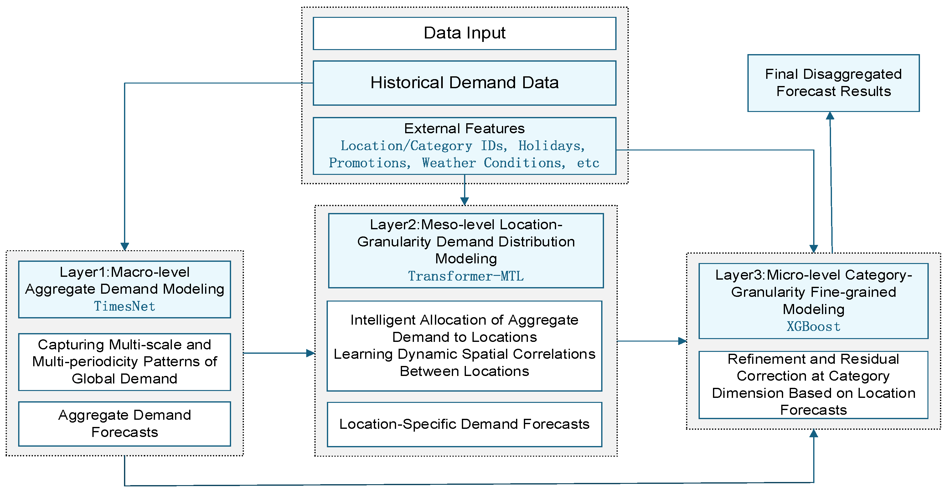
Figure 1 shows the framework of the H2SDF model. This model consists of three heterogeneous predictive modules and their inter-layer coupling mechanisms, enabling targeted modeling of macro, meso, and micro dynamic patterns embedded in fresh demand data. The innovation of this framework primarily manifests in the deep integration of hierarchical decomposition and heterogeneous model ensemble across two dimensions. At the macro layer, aggregate demand exhibits high signal-to-noise ratios and pronounced multi-scale periodicity; TimesNet was therefore chosen for its frequency-domain modeling capability and its effectiveness in decoupling nested temporal patterns via 2D convolutional structures. At the meso layer, spatial dependencies among locations are dynamic and non-Euclidean, driven by latent functional relationships rather than static geographical proximity. The Transformer encoder, with its self-attention mechanism, learns such dependencies directly from data without imposing rigid adjacency priors, and the multi-task learning framework enables parameter sharing while preserving location-specific prediction heads. At the micro layer, category-level series are sparse, noisy, and highly sensitive to contextual covariates. XGBoost, as a gradient-boosted tree ensemble, offers robust performance on heterogeneous tabular features and naturally accommodates the residual correction paradigm central to the micro-layer design.

The development of the H2SDF model is grounded in the distinct data characteristics and modeling requirements at each layer. At the macro layer, aggregate demand exhibits a high signal-to-noise ratio and pronounced multi-scale periodicity. This property favors a frequency-domain model that can explicitly decompose nested periodic patterns. TimesNet was therefore adopted for its ability to extract dominant frequencies and jointly model intra- and inter-period variations via 2D convolutions. In contrast, conventional recurrent architectures would be limited by long-term dependency degradation, while standard Transformers lack an explicit mechanism for multi-period decoupling. At the meso layer, spatial dependencies among locations are dynamic and driven by latent functional relationships rather than fixed geographical proximity. In order to capture such dependencies, a Transformer encoder with multi-head self-attention was employed. Graph neural networks (e.g., GCN, GAT) were avoided in this layer because they require a predefined adjacency matrix to govern message passing, which contradicts the objective of modeling evolving, functionally determined spatial influences. At the micro layer, category-level demand series are sparse, noisy, and sensitive to heterogeneous contextual covariates. This setting calls for a model that is robust to tabular features and can naturally perform residual correction on upstream forecasts. XGBoost was selected because gradient-boosted tree ensembles handle high-dimensional mixed-type features efficiently and iteratively learn residuals, aligning with the micro layer’s task of refining fine-grained errors. A pure deep learning stack was not adopted at this layer, as it would be more prone to overfitting on sparse series and less computationally efficient for the required per-location–category model instantiation.

(1)

Layer 1: Macro-Level Modeling Function. The first layer focuses on capturing global temporal trends and multi-scale periodicity from aggregate demand data:

$${\mathrm{f}}^{\left(1\right)}:{\mathrm{X}}_{\mathrm{t}\mathrm{o}\mathrm{t}\mathrm{a}\mathrm{l}}\to {\mathrm{R}}^{\mathrm{h}}$$

(2)

where ${\mathrm{X}}_{\mathrm{t}\mathrm{o}\mathrm{t}\mathrm{a}\mathrm{l}}$ represents the historical total demand sequence aggregated across all locations and categories, along with corresponding temporal features. The output $\widehat{{\mathrm{Y}}_{\mathrm{t}}^{\left(1\right)}}$ provides a smooth baseline trend that serves as a global constraint for subsequent layers.

(2)

Layer 2: Meso-Level Spatial Decomposition Function. The second layer decomposes the macro-level forecast into location-specific predictions while explicitly modeling spatial dependencies:

$${\mathrm{f}}^{\left(2\right)}:{\mathrm{X}}_{\mathrm{t}\mathrm{o}\mathrm{t}\mathrm{a}\mathrm{l}},{\mathrm{f}}^{\left(1\right)}\left({\mathrm{X}}_{\mathrm{t}\mathrm{o}\mathrm{t}\mathrm{a}\mathrm{l}}\right),{\mathrm{X}}_{\mathrm{s}\mathrm{p}\mathrm{a}\mathrm{t}\mathrm{i}\mathrm{a}\mathrm{l}}\to {\mathrm{R}}^{\left|\mathrm{S}\right|\times \mathrm{h}}$$

(3)

where ${\mathrm{X}}_{\mathrm{s}\mathrm{p}\mathrm{a}\mathrm{t}\mathrm{i}\mathrm{a}\mathrm{l}}$ includes location-specific historical demand sequences and spatial identifiers. This layer takes the first layer’s output as a reference signal, combines it with location-level contextual features, and produces demand predictions $\widehat{{\mathrm{Y}}_{\mathrm{s},\mathrm{t}}^{\left(2\right)}}$ for each location $\mathrm{s}\in \mathrm{S}$.

(3)

Layer 3: Micro-Level Category Refinement Function. The third layer performs final context-aware prediction corrections at the finest granularity:

$${\mathrm{f}}^{\left(3\right)}:{\mathrm{X}}_{\mathrm{t}\mathrm{o}\mathrm{t}\mathrm{a}\mathrm{l}},{\mathrm{f}}^{\left(1\right)}(·),{\mathrm{f}}^{\left(2\right)}(·),{\mathrm{X}}_{\mathrm{c}\mathrm{o}\mathrm{n}\mathrm{t}\mathrm{e}\mathrm{x}\mathrm{t}}\to {\mathrm{R}}^{\left|\mathrm{S}\right|\times \left|\mathrm{C}\right|\times \mathrm{h}}$$

(4)

where ${\mathrm{X}}_{\mathrm{c}\mathrm{o}\mathrm{n}\mathrm{t}\mathrm{e}\mathrm{x}\mathrm{t}}$ encompasses rich contextual features including local weather conditions, category attributes, promotional activities, and holiday indicators. This layer integrates outputs from both preceding layers and produces the final fine-grained forecasts $\widehat{{\mathrm{Y}}_{\mathrm{s},\mathrm{c},\mathrm{t}}^{\left(3\right)}}$ for each location–category combination.

This hierarchical structure ensures task-specific decomposition at different spatiotemporal scales, enabling each layer to concentrate on modeling patterns at its designated granularity level. The framework’s innovation lies in matching optimal algorithmic components to each sub-problem while maintaining coherence through inter-layer information flow.

2.4. Layer 1: TimesNet for Macro-Level Temporal Modeling

At the macro level of H2SDF, forecasting total demand provides the system-level reference that anchors downstream location-level disaggregation and category-level refinement. Fresh cold-chain demand is characterized by pronounced non-stationarity, nested multi-scale seasonality, and abrupt holiday-induced perturbations, which often weaken the robustness and generalization of conventional temporal models. To obtain a stable yet responsive macro forecast, we adopt TimesNet as the first-layer predictor. In this framework, TimesNet is used primarily for its ability to capture dominant periodic structures while remaining sensitive to localized anomalies, producing smooth baseline forecasts that are subsequently propagated as constraints/signals to the meso and micro layers. Specifically, TimesNet introduces frequency-aware period extraction and combines it with convolutional feature extraction to model both long-range periodic patterns and short-term deviations, mitigating the long-horizon dependency degradation seen in recurrent architectures and reducing the single-period bias that can arise in strictly single-scale models. Moreover, its frequency-based pathway provides a degree of structural transparency that is helpful for downstream analysis and abnormal-demand diagnosis, which aligns with the system-level role of the macro layer. Following the standard TimesNet design, the model stacks multiple TimesBlocks to progressively encode higher-order representations, where each TimesBlock implements a period perception–local pattern extraction–global integration process [25]. Given an input multivariate sequence ${\mathrm{X}}_{1\mathrm{D}}^0\in {\mathrm{R}}^{\mathrm{T}\times \mathrm{d}}$ with length T and feature dimension d, the stacked TimesBlocks output macro-level demand predictions for the next H time steps, which are then used to guide the subsequent hierarchical decomposition and residual adjustment stages. The internal process of TimesBlock comprises four key steps:

$$\mathrm{P}=\mathrm{F}\mathrm{F}\mathrm{T}\left({\mathrm{X}}_{1\mathrm{D}}^{\mathrm{l}-1}\right),{\left\{{\mathrm{w}}_{\mathrm{i}}\right\}}_{\mathrm{i}=1}^{\mathrm{k}}=\mathrm{T}\mathrm{o}\mathrm{p}\mathrm{K}\left(\left|\mathrm{P}\right|\right)$$

(5)

where ${\mathrm{w}}_{\mathrm{i}}$ represents the $\mathrm{i}$-th period frequency, and the $\mathrm{T}\mathrm{o}\mathrm{p}\mathrm{K}$ operation selects the $\mathrm{k}$ most significant period components in the energy spectrum.

(1)

2D Transformation and Reshaping. For each period ${\mathrm{w}}_{\mathrm{i}}$, the sequence is segmented and constructed into a 2D structure:

$${\mathrm{X}}_{2\mathrm{D}}^{\mathrm{l},\mathrm{i}}\in {\mathrm{R}}^{{\mathrm{p}}_{\mathrm{i}}\times {\mathrm{m}}_{\mathrm{i}}\times \mathrm{d}},{\mathrm{p}}_{\mathrm{i}}=\mathrm{T}/{\mathrm{w}}_{\mathrm{i}}$$

(6)

The 2D structure enables the model to leverage 2D convolution operations to perceive variation trends in both horizontal (inter-period) and vertical (intra-period) directions, significantly enhancing the model’s joint modeling capability for high-frequency disturbances and low-frequency trends.

(2)

Multi-Scale Inception Convolution. Each ${\mathrm{X}}_{2\mathrm{D}}^{\mathrm{l},\mathrm{i}}$ is input into an Inception Block containing 2D convolutional kernels of different sizes (e.g., $1\times 1,3\times 3,5\times 5$) that extract multi-granularity local features in parallel:

$${\widehat{\mathrm{X}}}_{2\mathrm{D}}^{\mathrm{l},\mathrm{i}}=\mathrm{I}\mathrm{n}\mathrm{c}\mathrm{e}\mathrm{p}\mathrm{t}\mathrm{i}\mathrm{o}\mathrm{n}\left({\mathrm{X}}_{2\mathrm{D}}^{\mathrm{l},\mathrm{i}}\right)$$

(7)

(3)

Adaptive Aggregation. The 2D features processed by convolution are flattened and projected back to 1D sequences:

$${\widehat{\mathrm{X}}}_{1\mathrm{D}}^{\mathrm{l},\mathrm{i}}=\mathrm{F}\mathrm{l}\mathrm{a}\mathrm{t}\mathrm{t}\mathrm{e}\mathrm{n}\mathrm{P}\mathrm{r}\mathrm{o}\mathrm{j}\left({\widehat{\mathrm{X}}}_{2\mathrm{D}}^{\mathrm{l},\mathrm{i}}\right)$$

(8)

Then, through an attention mechanism, weighted fusion is performed on representations under multiple period paths, ultimately outputting

$${\mathrm{X}}_{1\mathrm{D}}^{\mathrm{l}}={\displaystyle \sum _{\mathrm{i}=1}^{\mathrm{k}}}{\mathsf{\beta }}_{\mathrm{i}}{\widehat{\mathrm{X}}}_{1\mathrm{D}}^{\mathrm{l},\mathrm{i}},\mathsf{\beta }=\mathrm{s}\mathrm{o}\mathrm{f}\mathrm{t}\mathrm{m}\mathrm{a}\mathrm{x}\left({\mathrm{W}}_{\mathsf{\beta }}·\mathrm{G}\mathrm{A}\mathrm{P}\left(\mathrm{P}\right)+{\mathrm{b}}_{\mathsf{\beta }}\right)$$

(9)

where ${\mathsf{\beta }}_{\mathrm{i}}$ is the weight corresponding to the period, and GAP denotes global average pooling.

2.5. Layer 2: Transformer-Based Multi-Task Learning Model

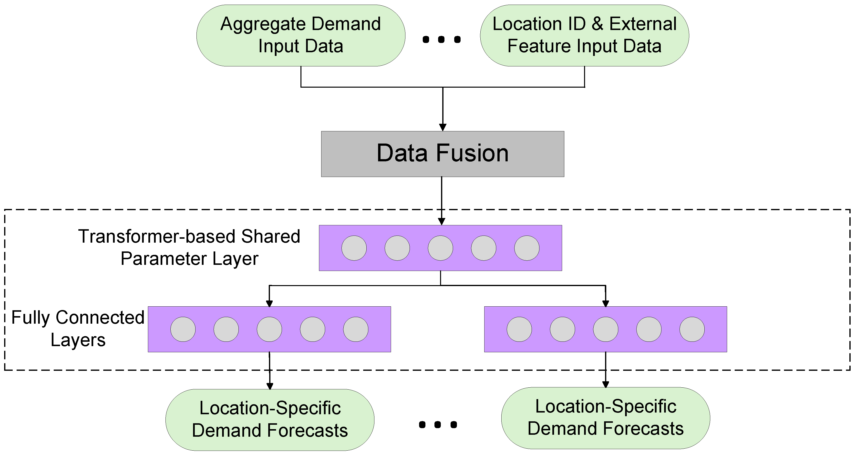
At the meso level of the H2SDF framework, the core task is to decompose the macro-level total demand prediction output from the first layer into each location according to its unique attributes and external features with spatial precision. To achieve this goal, this study designs a Transformer-based multi-task learning model aimed at simultaneously addressing two major challenges, independent demand modeling for each location and collaborative prediction among locations. The structural paradigm of this layer is shown in Figure 2. The model first learns common patterns and intrinsic associations of all locations through a shared bottom-layer feature extraction network, and then captures the unique demand patterns of each city using parallel, task-specific fully connected layers (i.e., prediction heads). To enhance the feature extraction capability of the shared layer, particularly to capture dynamic spatial associations among locations, this study employs the Transformer encoder as the core parameter-sharing module. The key advantage of the Transformer encoder lies in its multi-head self-attention mechanism, which enables the model to learn data-driven, dynamic “spatial association graphs” rather than relying on predefined static adjacency matrices.

Suppose there are $\mathrm{N}$ locations, each corresponding to a demand sequence ${\mathrm{X}}_{\mathrm{i}}\in {\mathrm{R}}^{\mathrm{T}\times \mathrm{d}}$, where $\mathrm{T}$ represents the time steps and $\mathrm{d}$ is the feature dimension at each step. Through a unified data encoding layer, all inputs are embedded and projected:

$${\tilde{\mathrm{X}}}_{\mathrm{i}}={\mathrm{X}}_{\mathrm{i}}·{\mathrm{W}}_{\mathrm{e}\mathrm{m}\mathrm{b}\mathrm{e}\mathrm{d}}+{\mathrm{b}}_{\mathrm{e}\mathrm{m}\mathrm{b}\mathrm{e}\mathrm{d}},\mathrm{i}=1,\dots ,\mathrm{N}$$

(10)

To achieve fine-grained modeling of demand at different locations, the model first treats each location as an independent prediction task and captures its uniqueness through the following mechanisms. The model’s input includes three parts: (1) the total demand prediction from the first layer; (2) external features at the current time step (such as weather, holidays, etc.); (3) the location ID representing the current prediction target. To enable the model to understand discrete location IDs, a location embedding layer is first employed to map each location’s ID into a low-dimensional, dense real-valued vector space. This embedding vector serves as a learned representation of each location’s unique characteristics. During training, the model automatically learns vector representations containing the intrinsic attributes of locations (such as population, economic level, and consumer consumption habits of the location).

After concatenating the total demand, external features, and location embedding vectors, the input data undergoes positional encoding to preserve sequential information and is then fed into multiple stacked encoder modules. Each module primarily consists of multi-head self-attention layers and feedforward neural networks. The core of the self-attention mechanism lies in its ability to allow the model, when processing information from one location (as Query), to simultaneously ‘see’ and evaluate information from all other locations in the dataset (as Keys and Values) [26].

All location inputs are then concatenated and fed into the shared Transformer encoder to obtain deep representations in the temporal dimension:

$${\mathrm{H}}_{\mathrm{i}}=\mathrm{T}\mathrm{r}\mathrm{a}\mathrm{n}\mathrm{s}\mathrm{f}\mathrm{o}\mathrm{r}\mathrm{m}\mathrm{e}\mathrm{r}\mathrm{E}\mathrm{n}\mathrm{c}\mathrm{o}\mathrm{d}\mathrm{e}\mathrm{r}\left({\tilde{\mathrm{X}}}_{\mathrm{i}}\right)$$

(11)

The multi-head self-attention mechanism is formulated as

$$\mathrm{A}\mathrm{t}\mathrm{t}\mathrm{e}\mathrm{n}\mathrm{t}\mathrm{i}\mathrm{o}\mathrm{n}(\mathrm{Q},\mathrm{K},\mathrm{V})=\mathrm{s}\mathrm{o}\mathrm{f}\mathrm{t}\mathrm{m}\mathrm{a}\mathrm{x}\left({\displaystyle \frac{{\mathrm{Q}\mathrm{K}}^{\mathrm{T}}}{\sqrt{{\mathrm{d}}_{\mathrm{k}}}}}\right)\mathrm{V}$$

(12)

where $\mathrm{Q},\mathrm{K},\mathrm{V}$ are the query, key, and value matrices, respectively, linearly mapped from the input ${\mathrm{H}}_{\mathrm{i}}$. Through this mechanism, the model can learn an implicit ‘spatial association graph’ in a data-driven and dynamic manner [27]. For example, the model might learn that the impact of promotional activities at location A on location B is greater than that of geographically closer location C. The multi-head mechanism allows the model to simultaneously learn multiple different association patterns from multiple perspectives (such as ‘competitive relationship’ and ‘complementary relationship’), greatly enhancing the model’s capability to capture complex spatial dependencies.

The attention outputs of multiple heads are concatenated and projected:

$$\mathrm{M}\mathrm{u}\mathrm{l}\mathrm{t}\mathrm{i}\mathrm{H}\mathrm{e}\mathrm{a}\mathrm{d}\left({\mathrm{H}}_{\mathrm{i}}\right)=\mathrm{C}\mathrm{o}\mathrm{n}\mathrm{c}\mathrm{a}\mathrm{t}\left({\mathrm{h}\mathrm{e}\mathrm{a}\mathrm{d}}_1,\dots ,{\mathrm{h}\mathrm{e}\mathrm{a}\mathrm{d}}_{\mathrm{h}}\right)·{\mathrm{W}}_0$$

(13)

Feedforward neural network layer:

$$\mathrm{F}\mathrm{F}\mathrm{N}\left(\mathrm{h}\right)=\mathrm{R}\mathrm{e}\mathrm{L}\mathrm{U}(\mathrm{h}·{\mathrm{W}}_1+{\mathrm{b}}_1)·{\mathrm{W}}_2+{\mathrm{b}}_2$$

(14)

After multiple layers of Transformer encoding, the model outputs task-specific predictions for each location. For the $\mathrm{i}$-th city, its output is

$${\widehat{\mathrm{y}}}_{\mathrm{i}}={\mathrm{f}}_{\mathrm{h}\mathrm{e}\mathrm{a}\mathrm{d}}^{\left(\mathrm{i}\right)}\left({\mathrm{H}}_{\mathrm{i}}\right)$$

(15)

where ${\mathrm{f}}_{\mathrm{h}\mathrm{e}\mathrm{a}\mathrm{d}}^{\left(\mathrm{i}\right)}$ represents the task-specific prediction head, typically composed of a set of fully connected layers. The final loss function adopts a multi-task weighted MSE loss:

$$\mathcal{L}={\displaystyle \sum _{\mathrm{i}=1}^{\mathrm{N}}}{\mathsf{\alpha }}_{\mathrm{i}}·{\Vert {\widehat{\mathrm{y}}}_{\mathrm{i}}-{\mathrm{y}}_{\mathrm{i}}\Vert }_2^2$$

(16)

where ${\mathsf{\alpha }}_{\mathrm{i}}$ is the task weight for city $\mathrm{i}$, and ${\mathrm{y}}_{\mathrm{i}}$ is its ground truth value.

2.6. Layer 3: XGBoost for Category-Level Fine-Grained Modeling

At the micro level of H2SDF, the goal is to generate final category-level forecasts by refining the meso-level location predictions, as this granularity directly supports SKU-oriented inventory and replenishment decisions and therefore requires high precision. We implement this layer with XGBoost regression, a robust gradient-boosted tree method for heterogeneous tabular features [28], and use it primarily as a category-specific residual corrector rather than a from-scratch forecaster. In contrast to the shared-parameter modeling adopted at upper layers, the micro layer follows a “divide-and-conquer” strategy to preserve category heterogeneity: we train an independent model for each location–category pair, allowing each sub-model to learn local nonlinearities such as category-specific consumption habits, seasonal sensitivities, and promotion responses. Each XGBoost model receives a fused feature vector that integrates multi-source hierarchical information, including (i) the macro-layer total-demand forecast as a global trend reference, (ii) the meso-layer location forecast as a locally grounded baseline after spatial dependency modeling, and (iii) contemporaneous contextual variables (e.g., temperature/precipitation, holiday indicators, promotion flags, workday type, and category attributes). By injecting the macro and meso predictions as structured inputs, the micro model focuses on learning the residual patterns and fine-grained fluctuations not fully captured by upstream deep models, thereby improving coherence and accuracy at the decision-critical category resolution. Operationally, the boosting procedure iteratively fits remaining errors across regression trees, yielding a strong predictor that systematically reduces residual variance and enhances final forecasting performance [29]. In mathematical expression, given training samples $\left({\mathrm{x}}_{\mathrm{i}},{\mathrm{y}}_{\mathrm{i}}\right)$, the XGBoost prediction value is

$${\widehat{\mathrm{y}}}_{\mathrm{i}}={\displaystyle \sum _{\mathrm{t}=1}^{\mathrm{T}}}{\mathrm{f}}_{\mathrm{t}}\left({\mathrm{x}}_{\mathrm{i}}\right),{\mathrm{f}}_{\mathrm{t}}\in \mathrm{F}$$

(17)

where $\mathrm{F}$ represents the set of all possible regression trees, ${\mathrm{f}}_{\mathrm{t}}$ is the structure and leaf weights of the $\mathrm{t}$-th tree, and $\mathrm{T}$ is the total number of trees. Its optimization objective is to minimize the following regularized loss function:

$$\mathcal{L}={\displaystyle \sum _{\mathrm{i}=1}^{\mathrm{n}}}\mathcal{l}\left({\mathrm{y}}_{\mathrm{i}},{\widehat{\mathrm{y}}}_{\mathrm{i}}\right)+{\displaystyle \sum _{\mathrm{t}=1}^{\mathrm{T}}}\mathsf{\Omega }\left({\mathrm{f}}_{\mathrm{t}}\right)$$

(18)

$$\mathsf{\Omega }\left(\mathrm{f}\right)=\mathsf{\gamma }\mathrm{T}+{\displaystyle \frac{1}{2}}\mathsf{\lambda }{\displaystyle \sum _{\mathrm{j}=1}^{\mathrm{T}}}{\mathrm{w}}_{\mathrm{j}}^2$$

(19)

where $\mathcal{l}\left(·\right)$ is the regression loss function (such as squared loss) and $\mathsf{\Omega }\left(·\right)$ is the structural regularization term used to control model complexity. The training process can be simplified into the following steps:

(1)

Initialize Model. First, the model starts from a very simple initial prediction, typically the mean of all training sample target values:

$${\mathrm{f}}_0\left(\mathrm{x}\right)=\mathrm{m}\mathrm{e}\mathrm{a}\mathrm{n}\left(\mathrm{y}\right)$$

(20)

(2)

Calculate Residuals. In each iteration round, the model calculates the difference between the current ensemble model’s predicted values and the true values, which is called residuals:

$${\mathrm{r}}_{\mathrm{i},\mathrm{t}}={\mathrm{y}}_{\mathrm{i}}-{\widehat{\mathrm{y}}}_{\mathrm{i},\mathrm{t}-1}$$

(21)

where ${\mathrm{r}}_{\mathrm{i},\mathrm{t}}$ is the residual of the $\mathrm{i}$-th sample in the $\mathrm{t}$-th round, ${\mathrm{y}}_{\mathrm{i}}$ is the true value, and ${\widehat{\mathrm{y}}}_{\mathrm{i},\mathrm{t}-1}$ is the cumulative prediction value of the first $\mathrm{t}-1$ rounds of models.

(3)

Fit Residuals. Next, the model trains a new, simple decision tree ${\mathrm{f}}_{\mathrm{t}}\left(\mathrm{x}\right)$, but this tree’s learning objective is no longer the original demand $\mathrm{y}$ but the residuals $\mathrm{r}$ calculated in the previous round. This means each new tree strives to learn and correct the errors collectively made by all previous trees:

$${\mathrm{f}}_{\mathrm{t}}\left(\mathrm{x}\right)\leftarrow \mathrm{f}\mathrm{i}\mathrm{t}\left({\mathrm{r}}_{\mathrm{i},\mathrm{t}}\right)$$

(22)

(4)

Update Model. The newly trained decision tree ${\mathrm{f}}_{\mathrm{t}}\left(\mathrm{x}\right)$ is multiplied by a learning rate $\mathsf{\alpha }$ to control the step size of each update and is added to the existing model to form a more powerful new ensemble model:

$${\widehat{\mathrm{y}}}_{\mathrm{i},\mathrm{t}}={\widehat{\mathrm{y}}}_{\mathrm{i},\mathrm{t}-1}+\mathsf{\alpha }{\mathrm{f}}_{\mathrm{t}}\left({\mathrm{x}}_{\mathrm{i}}\right)$$

(23)

(5)

Repeat Iteration. The model iteratively repeats steps (2) through (4), adding new decision trees to fit residuals until reaching the preset number of trees or when model performance no longer improves. The final prediction result is the sum of predictions from all decision trees.

2.7. Inter-Layer Coupling Mechanism

H2SDF is not a simple stack of three independent predictors; its key advantage is an inter-layer coupling mechanism that integrates heterogeneous models into a coordinated hierarchical system. The coupling is implemented as a top-down cascade of feature augmentation and progressive error correction: the macro layer provides a stable global forecast that is passed downstream as a compact, physically meaningful signal; the meso layer produces location forecasts conditioned on this global baseline and its learned spatial dependencies; and the micro layer refines category demand by learning residual patterns given both upstream forecasts and contextual covariates. Specifically, (i) top-down information flow injects higher-level predictions into lower-level models as core driving features, ensuring that each refinement step builds on aggregated spatiotemporal knowledge rather than restarting from scratch; (ii) constraint-guided coordination uses the macro forecast as a magnitude/trend anchor when modeling noisy location series, improving coherence across levels and reducing instability caused by local high-frequency fluctuations; and (iii) residual correction at the micro level fuses macro–meso outputs to isolate category-specific nonlinear deviations, helping the model focus on true demand drivers instead of random noise. Through this coupled pipeline, H2SDF achieves both hierarchical coherence and improved accuracy at decision-critical granularity. Meanwhile, unlike conventional reconciliation methods that enforce consistency post hoc, H2SDF integrates cross-level constraints directly into the training process, enabling the meso and micro layers to learn from macro-level signals rather than merely adjusting independent forecasts.

The prediction results satisfy hierarchical consistency constraints:

$$\sum _{\mathrm{s}\in \mathrm{S}}\widehat{{\mathrm{Y}}_{\mathrm{s},\mathrm{t}}^{\left(2\right)}}\approx \widehat{{\mathrm{Y}}_{\mathrm{t}}^{\left(1\right)}}+{\mathsf{ϵ}}_1$$

(24)

where ${\mathsf{ϵ}}_1$ is a bounded coupling error term. The total prediction error can be decomposed into independent contributions from each layer:

$${\mathrm{MSE}}_{\mathrm{total}}={\mathrm{MSE}}_{\mathrm{macro}}+{\mathrm{MSE}}_{\mathrm{spatial}}+{\mathrm{MSE}}_{\mathrm{category}}+{\mathsf{ϵ}}_{\mathrm{coupling}}$$

(25)

where ${\mathrm{MSE}}_{\mathrm{macro}}$ reflects deviation in the macro layer’s capture of overall trends, ${\mathrm{MSE}}_{\mathrm{spatial}}$ embodies error in the meso layer’s spatial distribution modeling, ${\mathrm{MSE}}_{\mathrm{category}}$ characterizes deviation in the micro layer’s category-specific fitting, and ${\mathsf{ϵ}}_{\mathrm{coupling}}$ represents coupling error in inter-layer information transfer. This decomposition indicates that the hierarchical architecture effectively reduces prediction errors of each component through specialized modeling, while the coupling error term approaches zero as inter-layer information transfer sufficiency increases, reflecting the theoretical advantages of collaborative modeling.

Table 1. Summary of Inputs and Outputs for Each Layer of the H2SDF Framework.

Layer	Model	Inputs	Outputs
Layer 1	TimesNet	Historical Total Demand Data	Total Demand Prediction Values
Layer 2	Transformer-MTL	Total Demand Prediction Values Current Time Step External Features Location IDs	Location-Specific Demand Forecasts
Layer 3	XGBoost	Total Demand Prediction Values Location-Specific Demand Forecasts Current Time Step External Features Location-Category IDs	Final Micro-level Category Forecasts

summarizes the inputs and outputs of each layer in the H2SDF framework, clearly illustrating the information flow and transformation process across the hierarchical structure. The first layer takes historical total demand data as input and outputs total demand prediction values. The second layer receives total demand prediction values, current time step external features, and location IDs as inputs, producing demand prediction values for each location. The third layer integrates total demand prediction values, location-level demand prediction values, current time step external features, and location-category IDs as inputs, yielding final micro-level category predictions.

In summary, through its unique inter-layer coupling mechanism, the H2SDF framework effectively integrates three heterogeneous models into a collaborative whole, achieving progressive prediction and refinement from macro to micro levels, providing a structurally clear and theoretically complete solution for solving complex multi-granularity demand prediction problems.

2.8. Parameter Configuration

The experiments were implemented using PyTorch 2.4.1 and executed on an environment with CUDA 11.8 acceleration. We set the historical look-back window (sequence length) to 24 time steps, and the batch size was configured to 256. For the macro layer (Layer 1), the hidden dimension was set to 128 with a dropout rate of 0.2 and a learning rate of 0.001. In the TimesNet module, the parameter k for extracting the top-k most significant period frequencies was set to 3, strategically capturing the dominant daily, weekly, and intra-day cycle variations in fresh product demand. At the meso layer (Layer 2), the Transformer-based multi-task learner utilized 8 parallel attention heads for the 128-dimensional hidden state. In order to mitigate overfitting on location-specific spatial heterogeneities, a dropout rate of 0.3 was applied. For the micro layer (Layer 3), the XGBoost residual corrector was configured with 100 estimators and a constrained maximum depth of 6 to avoid fitting high-frequency noise.

3. Case Study

The present study utilizes a real-world operational dataset from a large chain of fresh food supermarkets to validate model performance [30]. The dataset spans 124 days from 1 March to 2 July 2024, comprising a total of 2976 h timesteps across 18 geographically distributed nodes and 863 fresh product types. To standardize the modeling granularity and mitigate the influence of long-tail categories, an intelligent sales-volume-based weighted aggregation strategy was implemented, grouping the original 863 product types into 8 major categories based on their attributes. The dataset was split chronologically into training, validation, and test sets in a 6:2:2 ratio. This study focuses on single-step ahead forecasting (h = 1), predicting demand for the next hour based on historical hourly observations. This horizon aligns with the operational cadence of fresh cold-chain decision-making—such as replenishment for short-shelf-life products and workforce shift scheduling—while providing a rigorous baseline for evaluating the core architectural mechanisms of H2SDF.

To validate the effectiveness of the H2SDF hierarchical hybrid architecture, this study compares it against two representative baseline models. The first is the traditional statistical ARIMA model, serving as a classical benchmark for time series forecasting. The second is the advanced end-to-end deep learning model PatchTST, which excels at capturing long-term dependencies and represents the current state of the art. Comparative experiments are conducted independently at three hierarchical levels, total demand (macro layer), location-wise distribution (meso layer), and category granularity (micro layer), to comprehensively assess performance improvements across different aggregation scales.

To comprehensively evaluate the performance of the proposed three-layer spatiotemporal demand forecasting model, this study employs four key evaluation metrics: Root Mean Square Error (RMSE), Mean Absolute Error (MAE), Symmetric Mean Absolute Percentage Error (sMAPE), and the Coefficient of Determination (R²). Their mathematical formulas are, respectively, defined as follows:

$$\mathrm{R}\mathrm{M}\mathrm{S}\mathrm{E}=\sqrt{{\displaystyle \frac{1}{\mathrm{n}}}\sum _{\mathrm{i}=1}^{\mathrm{n}}{\left({\mathrm{y}}_{\mathrm{i}}-\widehat{{\mathrm{y}}_{\mathrm{i}}}\right)}^2}$$

(26)

$$\mathrm{M}\mathrm{A}\mathrm{E}={\displaystyle \frac{1}{\mathrm{n}}}\sum _{\mathrm{i}=1}^{\mathrm{n}}\left|{\mathrm{y}}_{\mathrm{i}}-\widehat{{\mathrm{y}}_{\mathrm{i}}}\right|$$

(27)

$$\mathrm{s}\mathrm{M}\mathrm{A}\mathrm{P}\mathrm{E}={\displaystyle \frac{100\mathrm{\%}}{\mathrm{n}}}\sum _{\mathrm{i}=1}^{\mathrm{n}}{\displaystyle \frac{\left|{\mathrm{y}}_{\mathrm{i}}-\widehat{{\mathrm{y}}_{\mathrm{i}}}\right|}{\left(\left|{\mathrm{y}}_{\mathrm{i}}\right|+\left|\widehat{{\mathrm{y}}_{\mathrm{i}}}\right|\right)/2}}$$

(28)

$${\mathrm{R}}^2=1-{\displaystyle \frac{\sum _{\mathrm{i}=1}^{\mathrm{n}}{\left({\mathrm{y}}_{\mathrm{i}}-\widehat{\mathrm{y}}\mathrm{i}\right)}^2}{\sum \mathrm{i}=1^{\mathrm{n}}{\left({\mathrm{y}}_{\mathrm{i}}-\overline{\mathrm{y}}\right)}^2}}$$

(29)

Here, ${\mathrm{y}}_{\mathrm{i}}$ denotes the observed value, $\widehat{{\mathrm{y}}_{\mathrm{i}}}$ represents the predicted value, $\overline{\mathrm{y}}$ is the mean of the observed values, and $\mathrm{n}$ is the sample size.

4. Results and Discussion

In order to evaluate the effectiveness of the proposed H2SDF framework across macro, meso, and micro, we conducted a series of experiments. We first compare the overall performance of H2SDF against key baseline models to establish its comprehensive superiority; subsequently, we detail the internal predictive performance of each hierarchical level within H2SDF to reveal the mechanism and effectiveness of its layered collaborative operation.

4.1. Overall Model Performance Comparison

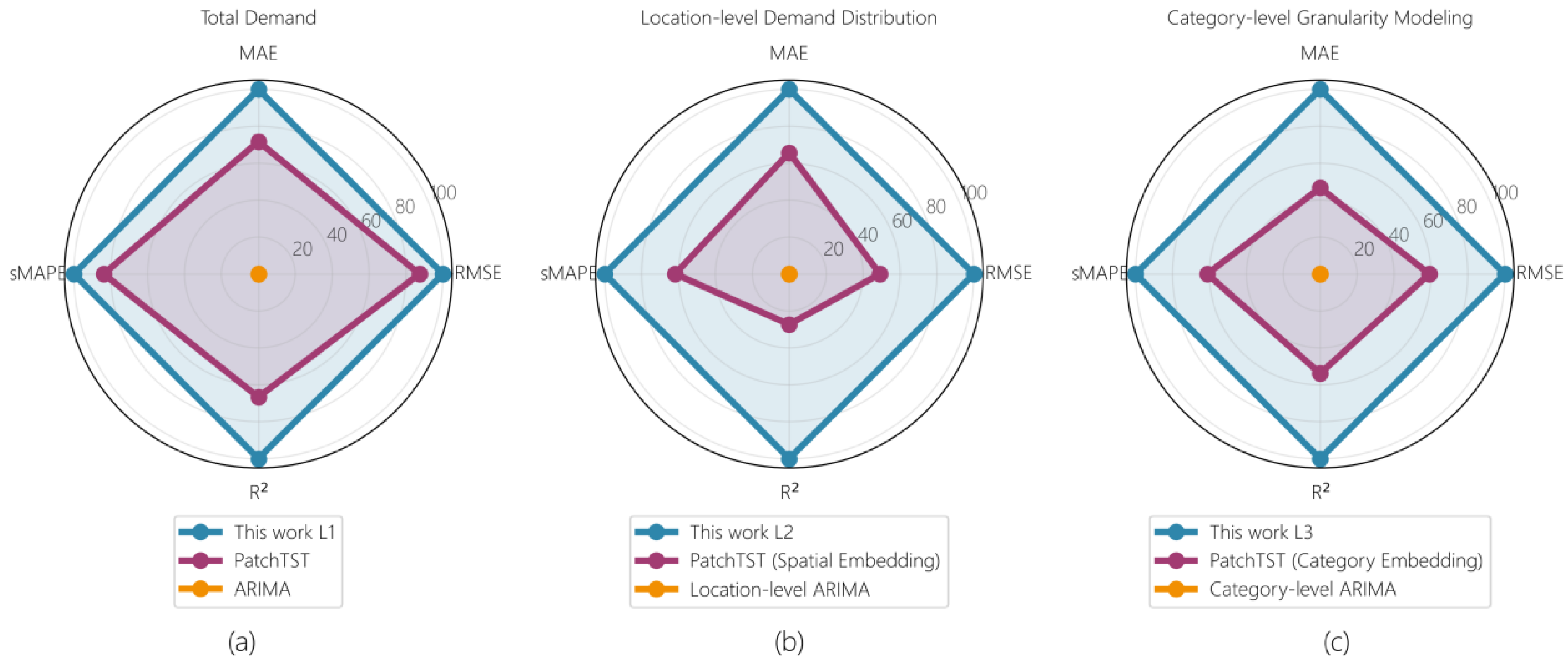
As shown in

Table 2. Model Comparison Results.

Model	RMSE	MAE	sMAPE	R2
H2SDF (Layer 1)	9.83	6.15	4.6%	0.99
PatchTST	10.31	6.88	5.2%	0.94
ARIMA	13.6	8.74	8.3%	0.86
H2SDF (Layer 2)	1.15	0.92	18.3%	0.90
Spatially Enhanced PatchTST	1.45	1.17	24.7%	0.82
ARIMA (Store Level)	1.74	1.65	35.1%	0.79
H2SDF (Layer 3)	0.22	0.16	22.4%	0.98
Category-Enhanced PatchTST	0.31	0.24	30.2%	0.91
ARIMA (Category Level)	0.44	0.31	42.5%	0.84

and Figure 3, the H2SDF framework consistently outperforms the two baseline models across all four evaluation metrics (RMSE, MAE, sMAPE, R²) at all three forecasting hierarchy levels, indicating its comprehensive predictive capability.

At the macro total demand level (Layer 1), H2SDF performs comparably to PatchTST, with both achieving an R² above 0.99, and both notably exceed ARIMA. This suggests that advanced deep learning models possess a distinct advantage in capturing complex long-term temporal trends, thereby laying a solid macro-level foundation for the forecasting task. The benefit of the hierarchical architecture becomes more evident at the meso location distribution level (Layer 2). The RMSE (1.15) and MAE (0.92) of H2SDF are lower than those of the spatially enhanced PatchTST. This indicates that as the forecasting task transitions from a univariate time series to a complex spatiotemporally coupled problem, the specialized modeling of H2SDF (Transformer-MTL) exhibits a structural advantage over generic end-to-end models. The traditional ARIMA model yields the highest error at this granularity, with an sMAPE of 35.1%, reflecting its difficulty in handling spatial heterogeneity among locations.

The advantage of H2SDF is most pronounced at the micro category granularity level (Layer 3). As reported in Table 2, H2SDF achieves an RMSE of 0.22 and an MAE of 0.16, providing precise fine-grained forecasts. In comparison, the RMSE of the category-enhanced PatchTST model (0.31) is 41% higher, while the RMSE of the category-level ARIMA model (0.44) is 100% higher. The magnitude of these errors in the baseline models limits their utility for refined inventory or replenishment decisions. This outcome highlights the importance of H2SDF’s progressive refinement and residual correction mechanism in handling high-noise, high-sparsity micro-granularity data. The radar chart in Figure 3 provides a visual comparison: the performance envelope of H2SDF (blue) extends further toward the outer ring across all three granularities, encompassing the profiles of both PatchTST and ARIMA on key error metrics RMSE and MAE, and illustrating the advantage of its hierarchical decoupling and specialized modeling strategy.

4.2. Detailed Hierarchical Performance of the H2SDF Framework

Having established the overall superiority of H2SDF, this section details the predictive performance of the framework’s internal three-layer models to validate the effectiveness of its progressive refinement and collaborative operation.

4.2.1. Layer 1: Macro-Level Total Demand Forecasting

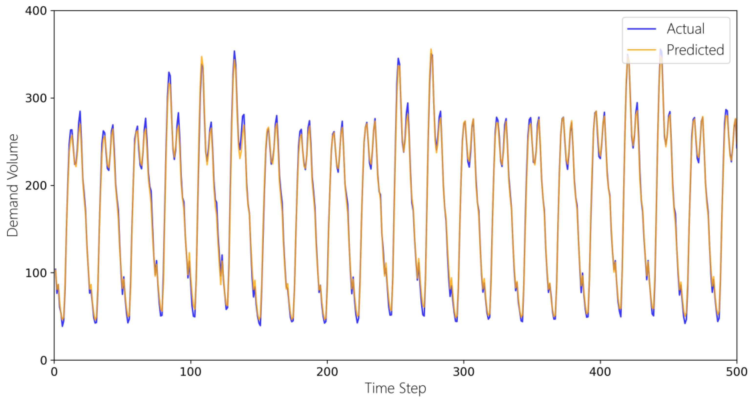
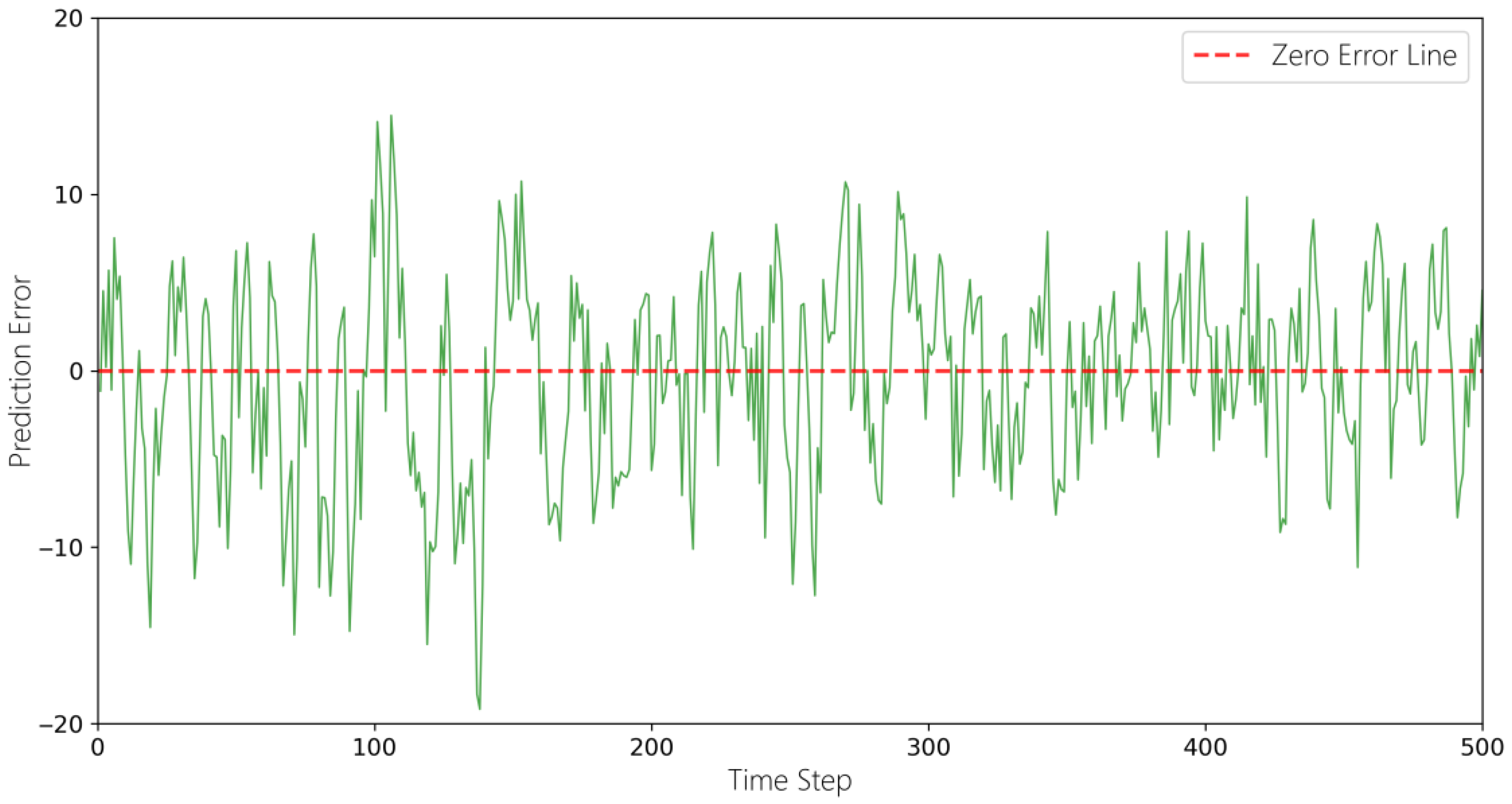
The TimesNet model in Layer 1 captures the macro-level temporal patterns of total network-wide demand. As shown in Figure 4, the forecasted curve (orange) aligns closely with the actual values (blue), tracking the periodic fluctuations, peaks, and troughs of demand. The model accurately fits both high-frequency intraday variations and weekly procurement peaks. The forecast error distribution in Figure 5 indicates that the majority of prediction errors fall within ±10 units, reflecting the stability and reliability of the model’s predictions. 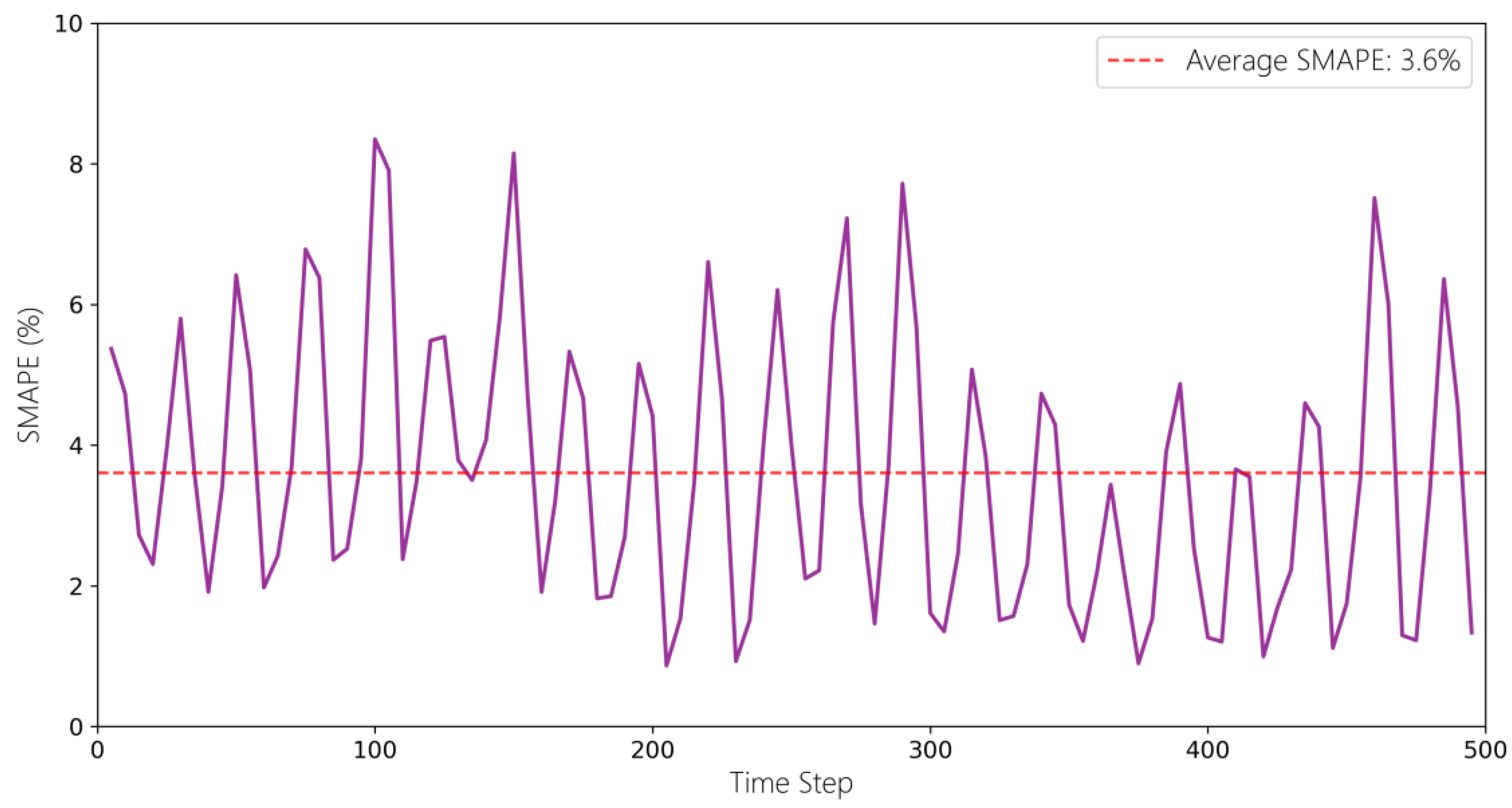As illustrated in Figure 6, forecast errors remain at a low level, with an average sMAPE of 3.6%. This strong macro-level performance can be attributed to the high signal-to-noise ratio of aggregated demand, which enables frequency-domain modeling to extract robust multi-scale trends without interference from local noise.

4.2.2. Layer 2: Meso-Level Location Demand Distribution

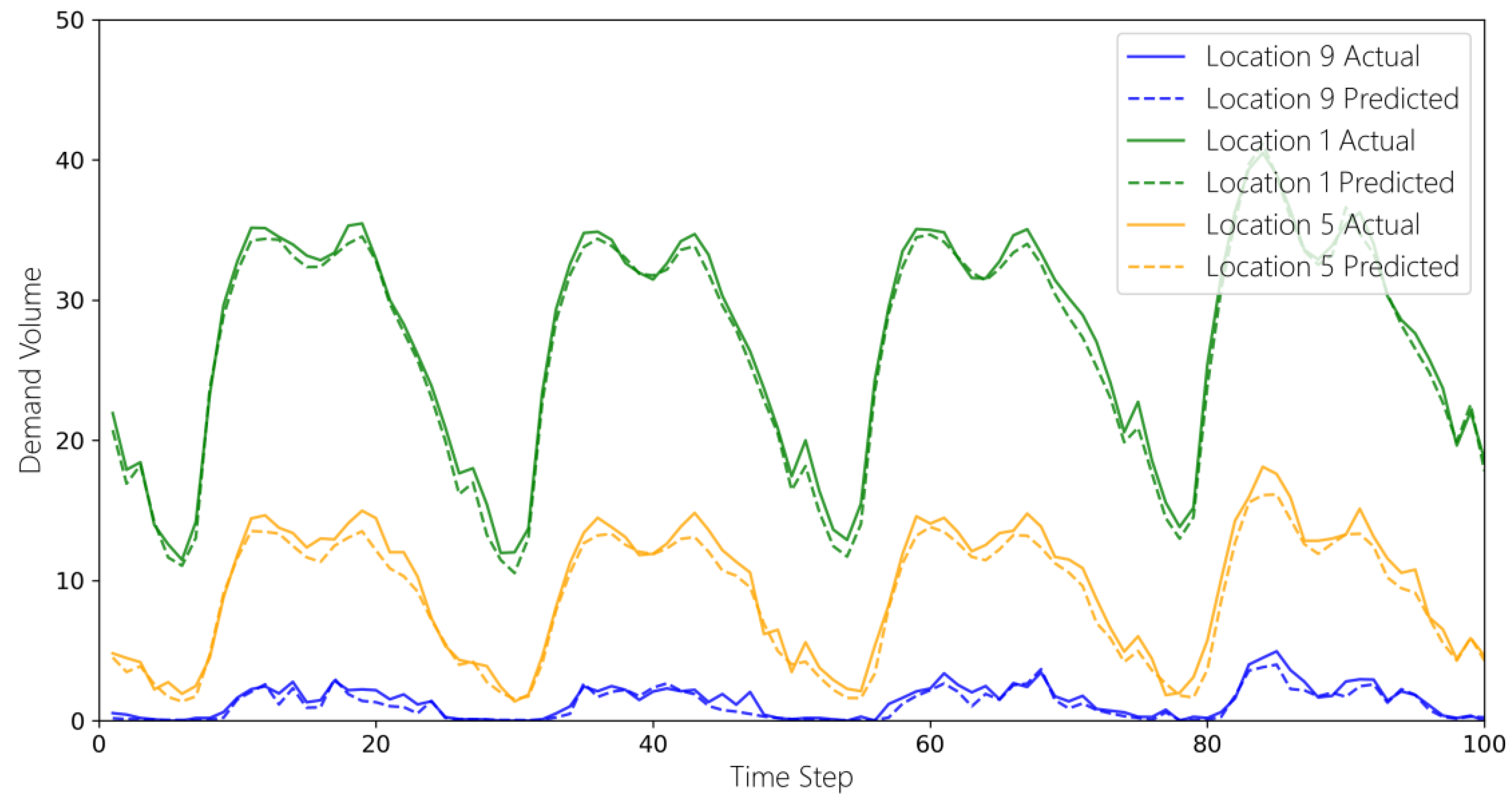
The Transformer-Multi-Task Learning (MTL) model in Layer 2 is tasked with decomposing the macro-level total demand forecast into predictions for 18 distinct locations while capturing the spatiotemporal heterogeneity among them. Figure 7 presents a comparative analysis between the forecasted and actual values for Location 1 (high demand), Location 5 (medium demand), and Location 9 (low demand), demonstrating the model’s robust predictive capability across locations with varying demand volumes. 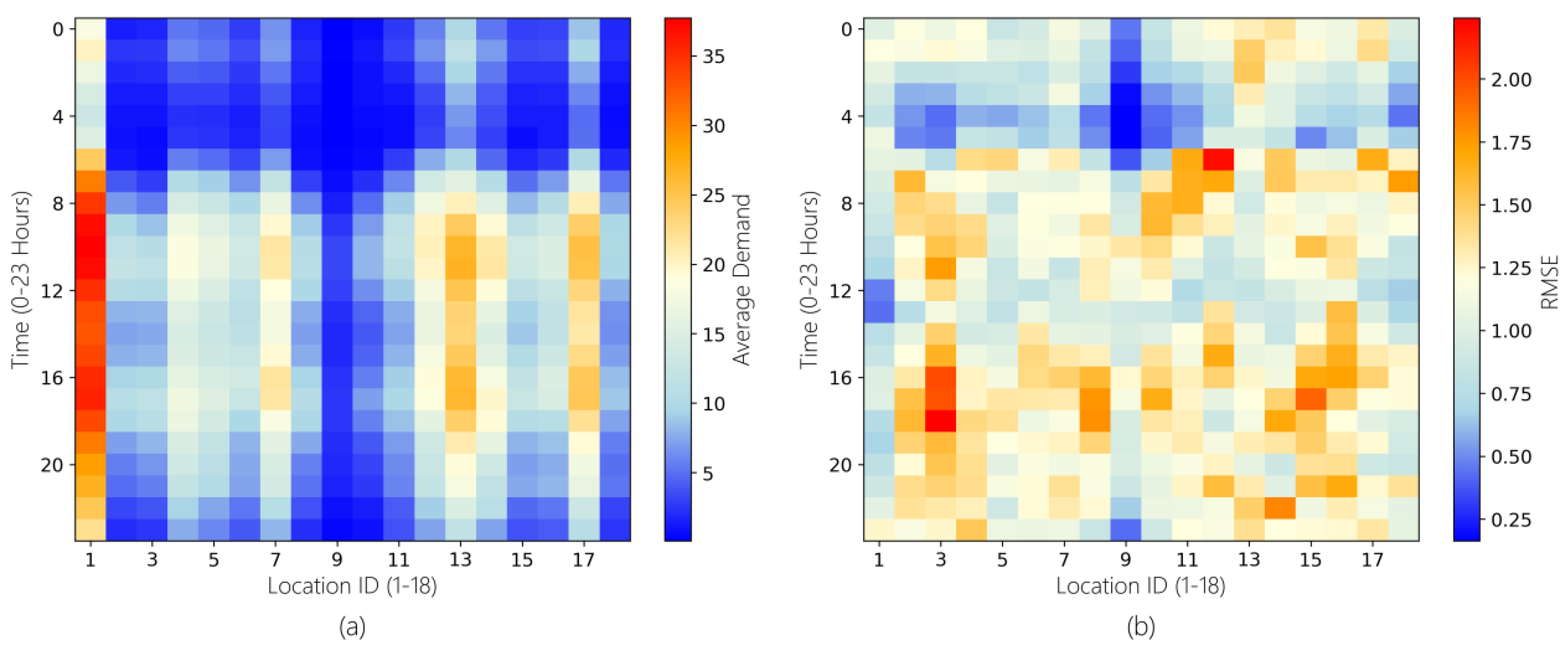The location–time cross-analysis heatmap in Figure 8 visually illustrates the model’s proficiency in spatiotemporal analysis. Specifically, Figure 8a clearly reconstructs the distinct demand patterns exhibited by different locations over a 24 h period (e.g., Location 1 shows high demand between 08:00 and 20:00, whereas Location 3’s demand is concentrated in the afternoon). This confirms the model’s sensitivity to spatial heterogeneity and offers data-driven support for formulating differentiated replenishment strategies across regions. The corresponding RMSE heatmap in Figure 8b indicates that prediction errors remain at a comparatively low level (mostly between 0.75 and 1.75) across the vast majority of spatiotemporal slices. Even under markedly different demand patterns across locations and time periods, the model’s predictive accuracy remains stable, with no notable performance degradation in any specific region. This robustness stems from the Transformer’s self-attention mechanism, which learns dynamic spatial dependencies directly from data without relying on predefined static graphs—an essential capability given that demand correlations across locations are often driven by functional similarities rather than mere geographical proximity.

4.2.3. Layer 3: Micro-Level Category Granularity Forecasting

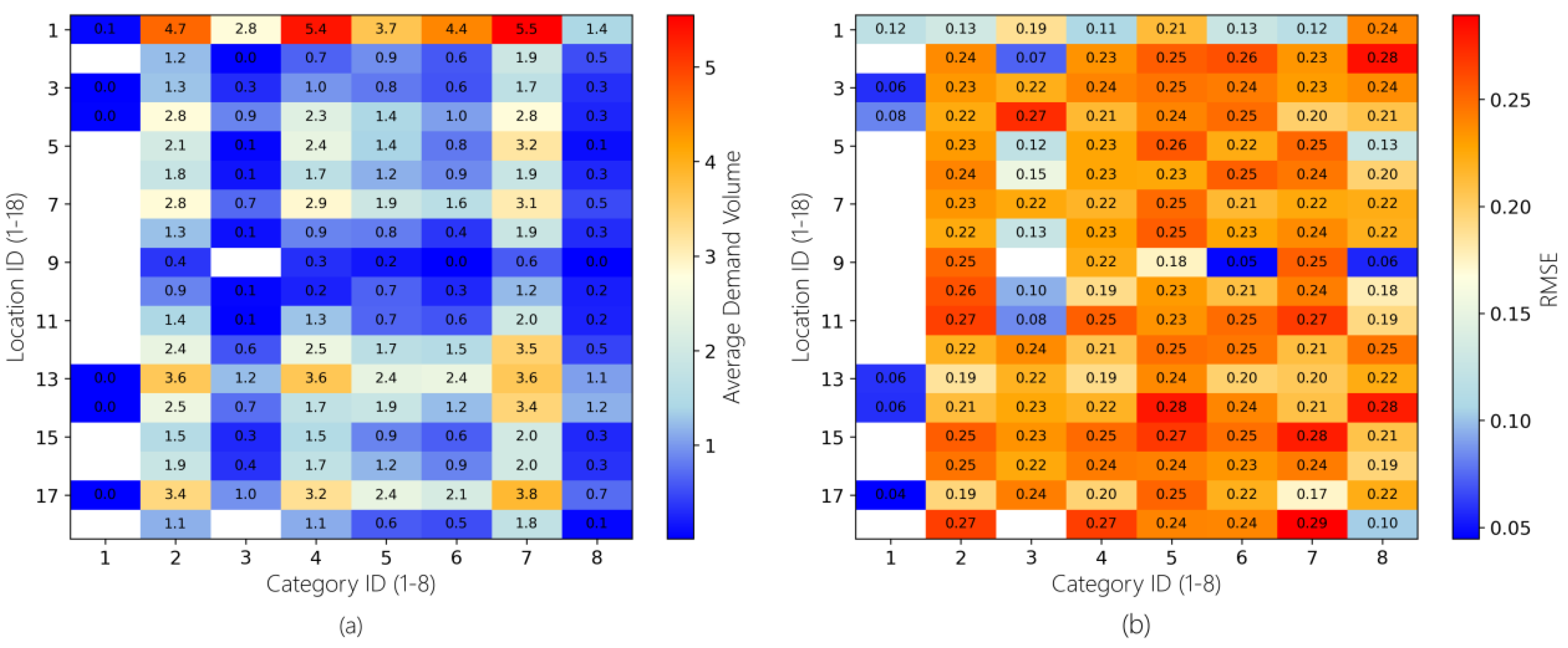
The XGBoost model in Layer 3 performs fine-grained residual correction for each location–category combination, building upon the macro-level trends (Layer 1 output) and meso-level distributions (Layer 2 output). This step translates forecasts into actionable insights for SKU-level decision-making. The location-category cross-analysis heatmap in Figure 9 illustrates predictive performance at this finest granularity. Figure 9a presents the demand matrix across 18 locations and 8 categories, while Figure 9b shows that the RMSE remains below 0.28 for nearly all combinations. This indicates that the XGBoost model effectively leverages the macro and meso features propagated from upper layers, filters out noise, and fits the nonlinear fluctuations driven by localized factors such as promotions and weather. The residual correction paradigm at this layer isolates category-specific nonlinear deviations, enabling XGBoost to focus on fine-grained variations that are not captured by upstream deep learning models. This task decomposition contributes to the framework’s overall accuracy at the decision-critical micro level.

4.3. Comprehensive Evaluation

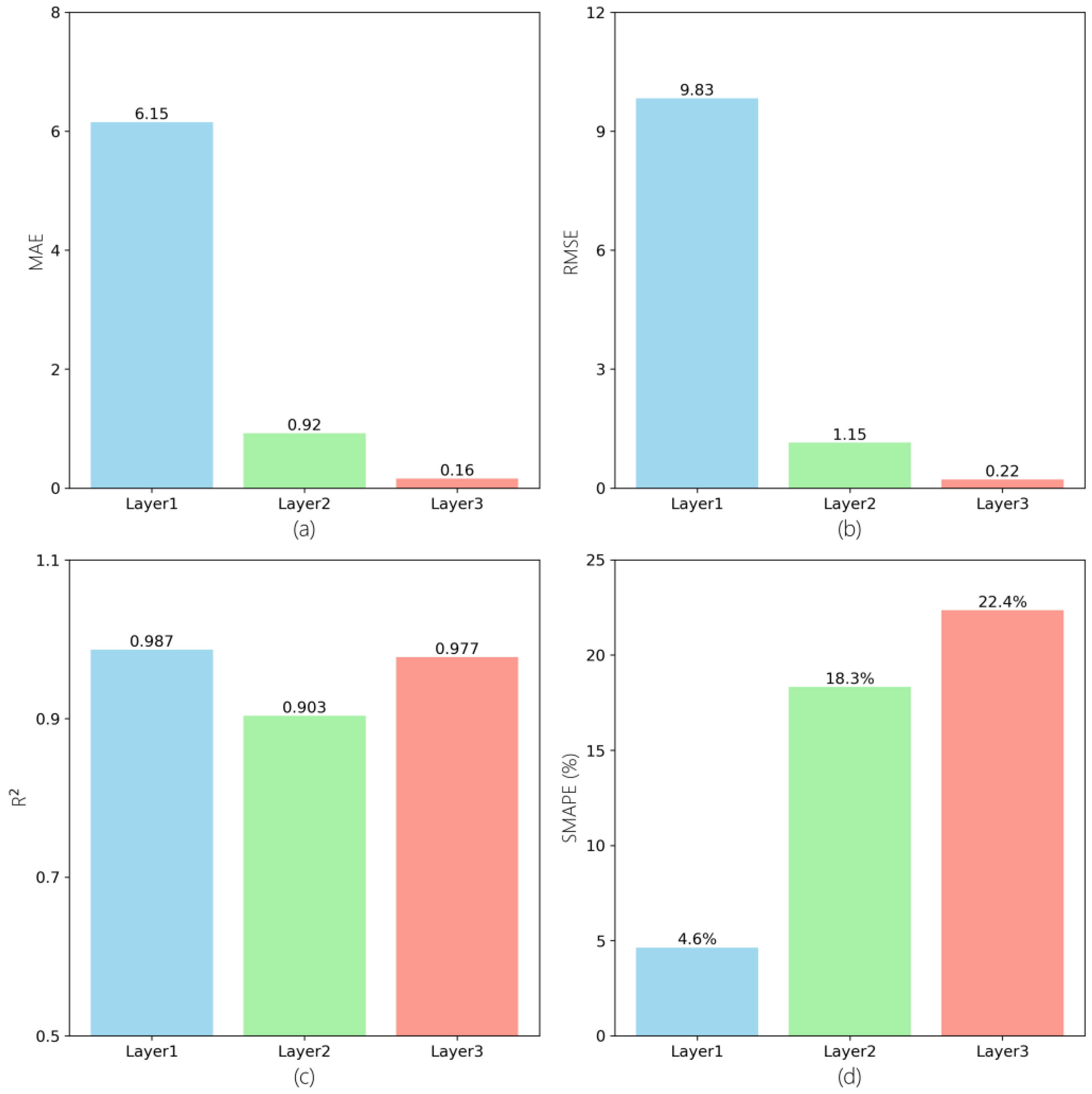
Figure 10 summarizes the progressive refinement effect of the H2SDF framework. From Layer 1 to Layer 3, the predictive granularity of the model is successively refined. Layer 1 achieves an R² value of 0.99, confirming its strong temporal modeling capability and its role in providing a reliable macro-level trend baseline for downstream layers. After introducing the spatial dimension, Layer 2 retains a robust R² value of 0.90, while MAE and RMSE decline to 0.92 and 1.15, respectively. This indicates that the model effectively captures spatial heterogeneity and performs a rational disaggregation of the macro-level aggregate. The refinement effect of Layer 3 is evident in the R² value rising to 0.98, with MAE and RMSE further reduced to 0.16 and 0.22, yielding strong predictive accuracy even on data characterized by high noise and sparsity. Throughout this process, MAE and RMSE decrease in proportion to the magnitude of the prediction target, demonstrating the model’s scale-adaptive capability. The R² value remains above 0.90 across all three levels, indicating that the model explains the vast majority of demand variance at each distinct scale and maintains high reliability.

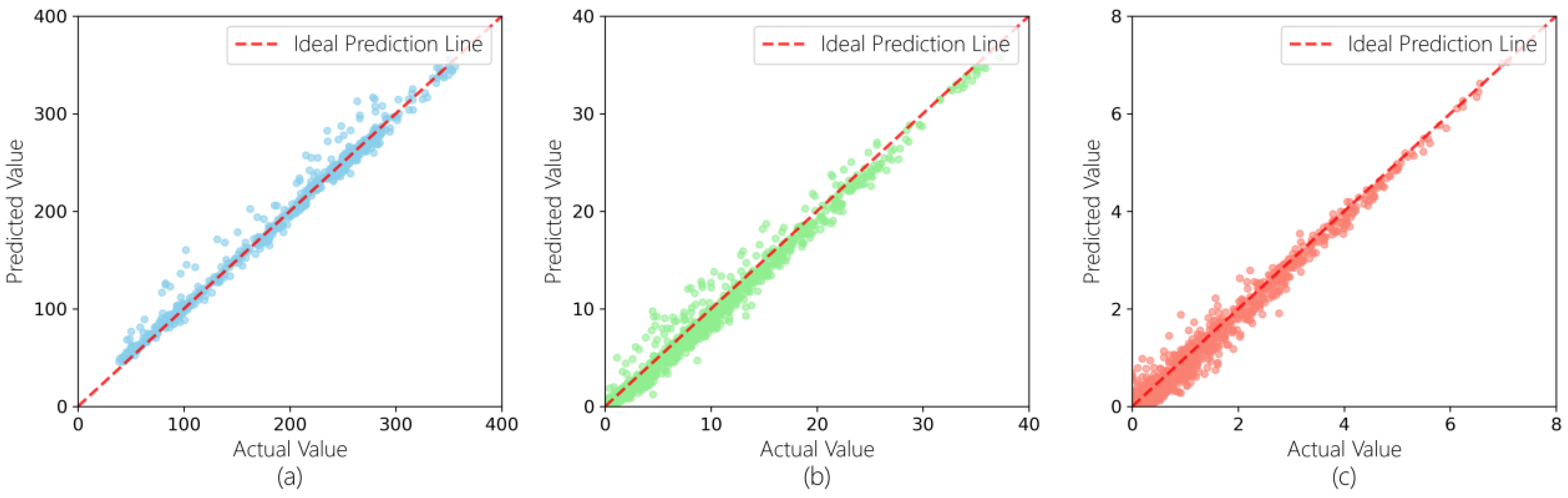
The scatter plots in Figure 11a–c further confirm the high consistency between the predicted and actual values across all three layers. All data points are tightly and uniformly distributed along the ideal prediction line, without exhibiting systematic overestimation or underestimation bias. This confirms the high accuracy, robustness, and unbiased nature of this hierarchical framework for the multi-granularity fresh cold chain demand forecasting task.

From an operational standpoint, these quantitative improvements carry tangible managerial implications. The reduction in RMSE at the micro level directly translates into lower safety stock requirements for short-shelf-life categories, thereby mitigating spoilage risk and reducing working capital tied up in inventory. The improved accuracy at the meso level supports more reliable workforce scheduling and distribution planning, as labor and vehicle assignments can be aligned more precisely with anticipated demand peaks.

These findings can be discussed with previous research on hierarchical forecasting and supply chain demand prediction. First, the results of the present study align with previous studies [22] in confirming that hierarchical architectures outperform flat, single-resolution models, as the former better accommodate the distinct statistical properties of demand at different aggregation levels. Second, this study finds that integrating heterogeneous models during the training phase can promote both accuracy and cross-level coherence. This demonstrates that information sharing across levels during model training constitutes a substantive advantage beyond what reconciliation alone can achieve. Third, previous studies predominantly rely on predefined static adjacency matrices to model inter-location relationships, while our results demonstrate that dynamic, self-attention-based spatial association learning better captures the functional and evolving dependencies that characterize real-world supply chain networks.

4.4. Ablation Study

To rigorously validate the contribution of each architectural component within the H2SDF framework, we conducted a comprehensive ablation study at the decision-critical micro-level (category granularity). We compared the full framework against three structurally degraded variants: (1) w/o Coupling, which trains the three layers independently without passing macro/meso features downstream; (2) w/o Layer 2, which replaces the embedding-based multi-task spatial allocation with a static historical-ratio distribution; and (3) w/o Layer 3, which removes the XGBoost category refinement layer, with category-level predictions instead obtained by disaggregating each location’s Layer 2 forecast according to that location’s historical average category proportions.

As shown in

Table 3. Ablation Study Results on Micro-level Category Forecasting.

Model Variants	Description	RMSE	MAE	sMAPE	R2
H2SDF (Proposed)	Complete three-layer coupled architecture	0.22	0.16	22.4%	0.98
w/o Coupling	Removed top-down feature flow (independent training)	0.26	0.19	25.8%	0.95
w/o Layer 2	Replaced meso-MTL with static historical ratio allocation	0.29	0.23	28.5%	0.92
w/o Layer 3	Removed XGBoost refinement	0.34	0.26	32.1%	0.89

, the complete H2SDF framework achieves the optimal performance (RMSE = 0.22). Removing any single component leads to a performance degradation. The w/o Layer 3 variant exhibits the most severe accuracy drop (RMSE increases by 54% to 0.34), confirming that upper-layer deep models alone struggle to capture the high-frequency, nonlinear noise inherent in category-level demand, thus proving the necessity of the gradient-boosted residual corrector. The w/o Layer 2 variant shows a decrease in R² (from 0.98 to 0.92), underscoring that static allocation fails to capture the dynamic spatial dependencies learned by our embedding-based multi-task mechanism. Even when all layers are present, cutting off the inter-layer information flow (w/o Coupling) increases the sMAPE, validating that the top-down constraint is crucial for maintaining hierarchical consistency and guiding micro-level predictions with macro-level trends.

5. Conclusions

This study introduces a Hierarchical Hybrid Spatio-Temporal Demand Forecasting (H2SDF) framework. Its primary contribution lies in proposing a system-level architectural solution to the problem of hierarchical forecasting under multi-granularity demand uncertainty, rather than an incremental enhancement to any single predictive model. H2SDF formulates multi-granularity forecasting as a hierarchical decomposition problem, aligning each layer’s modeling paradigm—frequency-aware temporal modeling, Transformer-based multi-task learning, and gradient-boosted residual correction—with the distinct statistical properties of aggregate, location-level, and category-level demand. An explicit top-down coupling mechanism propagates forecasts and consistency constraints across layers, enabling information sharing during training. This architectural design thus contributes to both forecasting theory and supply chain management knowledge by providing a generalizable blueprint for coordinating heterogeneous models across multiple decision granularities under demand uncertainty.

Experimental results on a real-world dataset spanning 2976 h observations across 18 locations and 8 product categories demonstrate that H2SDF consistently outperforms ARIMA and PatchTST baselines, achieving RMSE reductions of 12–41% across all three granularities. At the macro level, H2SDF attains an RMSE of 9.83 (10.31 for PatchTST and 13.6 for ARIMA); at the meso level, RMSE is 1.15 (1.45 and 1.74); and at the micro level, RMSE reaches 0.22 (0.31 and 0.44), with R² improving from 0.84–0.91 to 0.98. Several limitations warrant consideration: the data originate from a single retail enterprise, limiting generalizability; coupling errors during hierarchical transfer require further quantitative characterization. Future work will explore bidirectional coupling and multi-horizon validation to extend applicability across diverse supply chain contexts.

From a practical standpoint, adopting the H2SDF framework operationally can follow four steps. First, aggregate historical demand data to the three hierarchical levels and construct the required contextual features, including calendar variables, weather records, promotional calendars, and location–category attributes. Second, the macro-layer TimesNet model is trained on total demand to establish a stable system-level baseline. Third, the meso-layer Transformer-MTL model is trained using the macro forecasts, location identifiers, and external features to generate location-specific predictions. Fourth, per-location–category XGBoost models are trained on the fused upstream forecasts and contextual covariates to produce the final fine-grained predictions. The framework is beneficial under conditions where demand patterns exhibit pronounced multi-scale periodicities and non-stationarity, where spatial dependencies among locations are functional and dynamic, and where operational decisions depend on accurate forecasts at multiple granularities simultaneously.