Multi-Objective Route Planning for Sustainable Multimodal Hazardous Material Transportation: An Improved NSGA-II Approach with Entropy-Weighted TOPSIS Decision Making

Abstract

With the advancement of global industrialization, the market for the transportation of hazardous materials is also expanding, which poses an increasingly serious threat to public safety, environmental protection, and economic stability. This study explores solutions to improve the safety and sustainability of transportation by integrating a variety of transportation modes, such as highways, railways, and waterways. We have built a comprehensive assessment system that takes into account safety considerations, operating costs, and environmental impact. The methodological contributions include an improved NSGA-II algorithm featuring population invasion and homologous competition mechanisms, combined with entropy-weighted TOPSIS for objective route selection. We use the improved NSGA-II algorithm combined with the entropy weighted TOPSIS method to model the solution, screen the optimal scheme, and determine the actual feasible route. We used the real transportation route from Berlin to Paris as a case to verify the validity of the model and proved the improved effect of the algorithm by comparing it with the baseline NSGA-II and MOQPSO. The experimental results demonstrated that the improved algorithm achieved a 133% higher hypervolume than the baseline NSGA-II and 58.8% higher than MOQPSO, while the optimal solution reduced operating costs by approximately 7.3% and carbon emissions by 12.7%. The experimental results proved that the framework effectively reduced the accident rate, operating costs, and carbon emissions. The research results provide important references for logistics planners, fully demonstrating that under the increasingly complex world pattern, it is a feasible plan to improve the efficiency of hazardous materials transportation through multimodal transportation.

1. Introduction

With the continuous advancement of global industrialization, the scale of the hazardous materials market is also expanding, and the transportation of hazardous materials has become an important link in modern logistics. According to the relevant literature, it can be seen that the number of accidents in the transportation of hazardous materials has been on the rise in recent years, of which 41.7% occurred in the transportation stage, and 31.5% occurred in the transshipment stage, often accompanied by material leakage [1]. These accidents may have a far-reaching impact on many aspects, such as the environment, public safety, and the economy. Therefore, it is imperative to optimize the transportation of hazardous materials [2].

Multimodal transport integrates two or more modes of transportation (including highways, railways, and waterways) [3,4,5], and has become a key method to optimize the efficiency of hazardous materials transportation. And in practical application, the benefits of different modes of transportation must be comprehensively evaluated to determine the best solution [6]. For example, in the context of increasingly serious global climate change and environmental problems, the optimization of carbon emissions is often regarded as a key goal of multimodal transport path optimization [7,8,9,10,11]. Overall, multimodal transportation problems are typically regarded as multi-objective optimization problems, aiming to maximize comprehensive benefits and promote sustainable development by balancing multiple objectives. For example, Mehrem et al. [12] developed an optimization scheme for agricultural cold-chain logistics in multimodal transportation, using total transportation cost, refrigeration cost, and carbon emission costs from transportation and refrigeration as objective functions. Binsfeld et al. [13] established a model with total cost and carbon emissions as objectives. Recent studies have extended multimodal optimization to emerging delivery models. For instance, Lu et al. [14] proposed a joint delivery model integrating drones, occasional drivers, and riders for takeout routing optimization, achieving significant reductions in delivery time and operational costs under dynamic order scenarios.

Unlike single-mode transportation, which is limited by fixed routes, lower capacity, and higher environmental impact, multimodal transportation integrates two or more modes (road, rail, and waterway) and offers core advantages: (1) greater flexibility through mode switching at transshipment nodes; (2) higher carrying capacity; (3) significantly lower carbon emissions and accident risk per ton-kilometer; and (4) compliance with complex constraints such as regulatory bans and time windows. These characteristics make multimodal transportation particularly suitable for hazardous materials, enabling a better balance among safety, cost, and sustainability that single-mode systems cannot achieve.

The multimodal route optimization problem is an NP-hard problem; thus, after establishing the objective functions, optimization algorithms are required to validate the model’s effectiveness. Commonly used algorithms for multimodal route optimization include genetic algorithms (GA) [15], particle swarm optimization (PSO) [16], and ant colony optimization (ACO) [17,18]. Cui et al. [19] introduced fuzzy decision-making to improve the NSGA-III algorithm for solving a multi-objective multimodal transportation route optimization (MTRO) model. Zhang et al. [20] proposed a multi-objective weighted sum Q-learning optimization framework, incorporating an undirected multi-node network and representing time uncertainty with a positively skewed distribution. Ru [21] employed a tabu search algorithm to optimize a multimodal route model and demonstrated its superior performance through comparisons with other algorithms. Faroqi [22] utilized the NSGA-II multi-objective optimization algorithm to validate the model and confirmed its practicality via algorithm performance comparisons. Qi [23] integrated improved mutation operators, crowding distance calculations, and the C-W saving algorithm into the NSGA-II framework to solve for the optimal transportation path, further leveraging ArcGIS software for shortest path planning in real-world road networks. Prakash et al. [24] An innovative method is proposed to use artificial intelligence (AI) to predict the path in the multimodal transport network by combining Monte Carlo simulation and an LSTM network, highlighting the cutting-edge achievements of the sustainable development of this field. Farahmand-Tabar [25] uses the multi-objective quantum particle group optimization (MOQPSO) method to solve the path planning problem in urban transportation networks. Through comparative experiments, it is shown that the Pareto decompression quality generated by the MOQPSO algorithm is significantly better than that of the MOPSO and NSGA-II algorithms. Feng [26] verified the validity of the model through numerical experiments to simulate real scenes and, finally, obtained the optimal transportation scheme. These studies reveal a rich multi-objective algorithm system to solve the multimodal route optimization model, which requires us to choose the appropriate algorithm according to the specific model to obtain the optimal solution.

Relevant scholars have carried out a series of studies on the optimization of the multimodal transport route of hazardous materials. For example, Myronenko et al. [27] published a high-quality review article exploring the multimodal logistics chain in the international transportation of hazardous materials and perishable goods, especially emphasizing the application of emergency logistics in crisis situations. The author pointed out that the traditional single mode of transportation is often difficult to meet the needs of rapid and efficient response in disasters, crises, or military conflicts. Thus, they advocate multimodal approaches to enhance flexibility, cost-effectiveness, and resilience, especially for hazardous materials. Liu et al. [28] proposed a novel time-varying route optimization model for hazardous materials transportation incorporating risk equity considerations and designed an improved genetic algorithm based on the $\epsilon$-constraint method to validate the model. Chen [29] introduced a multimodal network and multi-criteria route optimization method, first constructing a three-objective integer programming model and then employing an improved multi-objective genetic algorithm, DSNSGA3, to support decision-making.

In summary, existing research on multimodal route optimization is abundant. However, few studies integrate multimodal methods for hazardous materials transportation. Therefore, this paper optimizes multimodal transportation in the context of hazardous materials by first constructing a three-objective model incorporating risk, cost, and carbon emissions. Second, an improved NSGA-II algorithm is used to solve the model and validate its effectiveness. After obtaining the Pareto front, entropy-weighted TOPSIS is applied to determine the optimal path, with the model’s validity further verified through a real-world case scenario from Berlin to Paris.

2. Model Formulation

2.1. Problem Description

The transportation of hazardous materials poses a major challenge to the sustainable logistics system. This challenge is particularly prominent in the multimodal transport network. It is mainly manifested in the need to integrate multiple modes of transportation in order to improve efficiency, ensure safety, and meet environmental protection requirements. However, hazardous materials, such as chemicals, fuels, and radioactive substances, need to be treated professionally. Once an accident occurs, it will cause serious harm to human health, the ecological environment, and infrastructure.

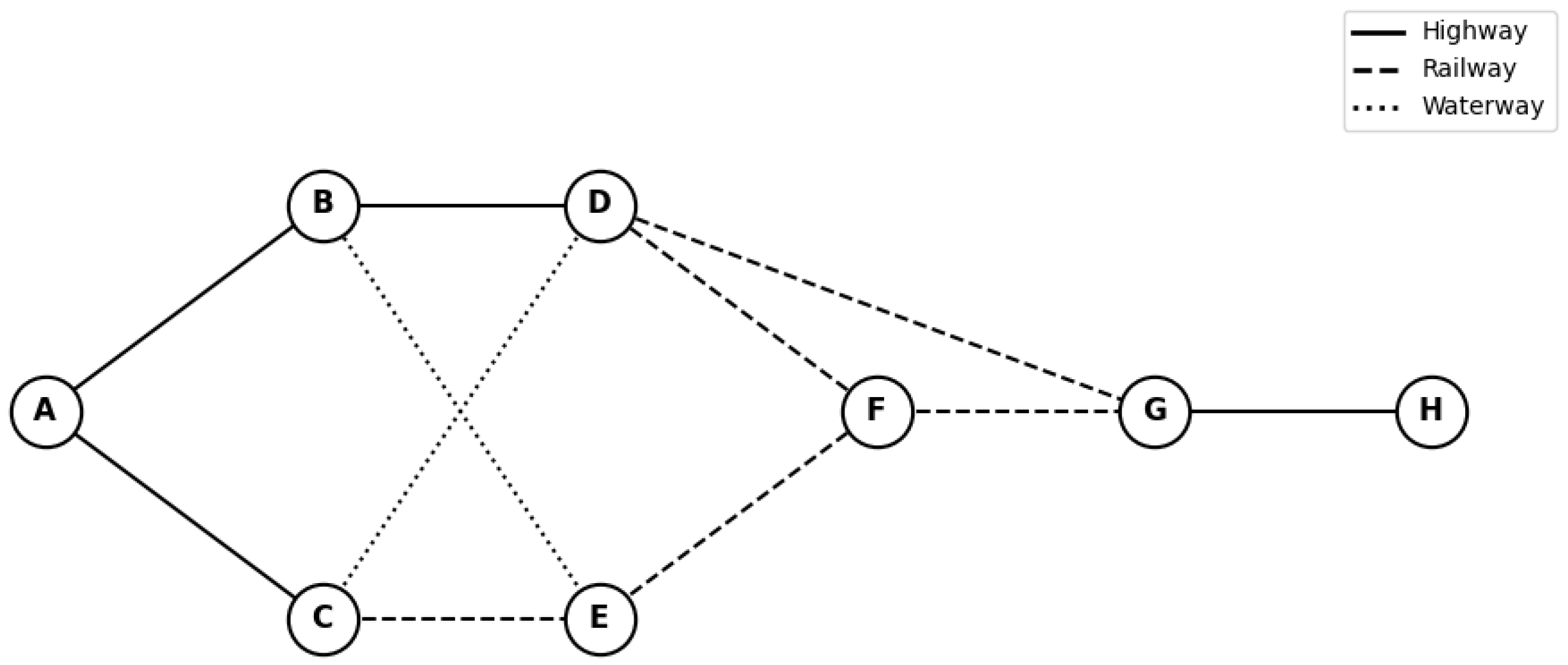
Assume that a batch of hazardous materials is transported from City A to City H, with the entire transportation network comprising multiple nodes. Figure 1 illustrates a schematic diagram of the random path layout network for multimodal transportation [30]. As shown in the figure, there are six nodes between City A and City H: B, C, D, E, F, and G. Three different transportation modes are available between each node. We evaluate transportation and transshipment safety risks between nodes. Then, we compare carbon emissions and costs for the three modes. This determines the optimal combination scheme, completing the multimodal plan for hazardous materials from City A to City H.

In research on multimodal route optimization for hazardous materials transportation, the core issues to be addressed can be summarized as follows: First, we must quantify and model safety risks. Second, we must employ safety risks, transportation costs, and carbon emissions as optimization objective functions. We must also incorporate regulatory prohibitions, carbon emissions limits, transportation time windows, and transportation modes as constraints to achieve safe hazardous materials transportation by balancing multi-objective conflicts.

2.2. Model Hypothesis

To lay a solid foundation for building the proposed multi-objective optimization model, this paper adopts five key assumptions. These assumptions simplify the complex reality in the transportation of hazardous materials while retaining the essential characteristics of the problem.

The setting of these five assumptions aims to strike a balance between the ease of handling of the model and the practical application value. By setting deterministic parameters and homogeneous goods, the model can concentrate computing resources on the core multi-objective trade-offs (risk, cost, and emissions) while maintaining compatibility with actual regulatory requirements and time window constraints. The specific assumptions are as follows:

(1) The transportation network is modeled as a directed graph with fixed nodes and connections. Each connection supports one or more predefined modes of transportation, and there will be no dynamic changes during the planning period [31].

(2) Hazardous materials are regarded as single and homogeneous commodities. Its total amount Q is fixed, and it is assumed that there is no separability problem or partial loss (except for the risk of modeling only) [32].

(3) All parameters, including distance, cost, emission factor, accident probability, and severity, are determined and known a priori. Carbon emissions and safety risks are linearly proportional to the transportation volume and driving distance. At the same time, ignore nonlinear effects such as congestion or variable weather effects [33].

(4) Transshipment is only carried out at the specified node, and it is only possible when switching the compatibility mode. The relevant risks and costs will be accumulated to the overall objectives [34].

(5) The time window and regulatory prohibitions are strictly enforced, and violations are not allowed. Moreover, the model assumes full compliance and no random delay [35].

Although the current model adopts deterministic parameters to improve computing efficiency, under real conditions, the probability of accidents $p_{ij}^m$ and the severity $s_k$ are inherently random and are affected by uncertainty factors (such as weather and traffic density). Future research expansion can introduce random variables or fuzzy sets to further improve the authenticity of the model.

All indices and variables in the following equations are defined in

Table 1. Summary of model notation.

Symbol Indices	Description
$i,j$	Nodes in the transportation network
$m,n$	Transportation modes (1 = road, 2 = rail, 3 = waterway)
k	Type of hazard or consequence severity category
$q_{ij}^m$	Quantity of hazardous materials transported from node i to j using mode m
$x_{ij}^m$	Binary indicator: 1 if link from i to j using mode m is selected, 0 otherwise
$y_i^{mn}$	Binary indicator: 1 if transshipment occurs at node i from mode m to n, 0 otherwise
Q	Total quantity of hazardous materials to be transported from origin to destination
$d_{ij}^m$	Distance of link from i to j using mode m
$p_{ij}^m$	Accident probability on link i to j using mode m
$p_i^{mn}$	Accident probability during transshipment at node i from mode m to n
$s_k$	Severity score for hazard type k
$c_{ij}^m$	Unit transportation cost per km for link i to j using mode m
$c_i^{mn}$	Unit transshipment cost at node i from mode m to n
${\mathrm{ins}}_k$	Insurance premium per unit quantity for hazard type k
$e_{ij}^m$	Emission factor per km per unit quantity for link i to j using mode m
$e_i^{mn}$	Emission factor per unit quantity during transshipment at i from m to n
$C^m$	Capacity limit for mode m (per link)
$s^m$	Speed of mode m (e.g., km/h)
${\mathrm{TW}}_{max},{\mathrm{TW}}_{min}$	Upper and lower bounds of the delivery time window (in hours)
${\mathrm{Ban}}_{ij}$	Binary indicator: 1 if link i to j is prohibited (regardless of mode), 0 otherwise
$m_{\mathrm{prev}},m_{\mathrm{curr}}$	Previous and current modes at a transshipment node

.

2.3. Mathematical Model

The model is a three-objective optimization framework. It aims to minimize safety risks, total costs, and carbon emissions, while integrating transportation and transit hub operations. Its objective functions are constructed as follows:

$$min\{f_1,f_2,f_3\}$$

All variables and indices appearing in the equations of Section 2.3 are explicitly defined in Table 1.

(1) Minimize safety risk:

Step 1: The formula for accident probability $p_i$ can be expressed as:

$$\begin{array}{c}\hfill p_i={\displaystyle \frac{N_{\mathrm{accidents}}}{D_{\mathrm{total}}}}\end{array}$$

(1)

where $N_{\mathrm{accidents}}$ is the number of historical accidents on the specific path segment i, and $D_{\mathrm{total}}$ is the total exposure.

For more complex scenarios, advanced methods can be employed to estimate the accident probability $p_i$, enhancing the model’s ability to handle uncertainty and mode-specific variations. Poisson regression or the negative binomial distribution can fit accident frequency as a function of influential variables such as traffic density. Such as:

$$p_i=exp({\beta }_0+{\beta }_1\times \mathrm{traffic}\mathrm{volume}+{\beta }_2\times \mathrm{weather}\mathrm{factor}),$$

(2)

where coefficients $\beta$ are estimated using MATLAB R2024b’s fitglm function. This approach accounts for over-dispersion in count data, common in transportation accidents.

If the data is insufficient, proxy variables can be used:

$$p_i=p_{\mathrm{general}}\times f_{\mathrm{hazard}}$$

(3)

Among them, $p_{\mathrm{general}}$ is the general freight accident rate, and $f_{\mathrm{hazard}}$ is the coefficient of hazardous materials, and the value range is 2 to 5.

Step 2: In order to assess the severity $s_i$, a quantitative method based on impact scale grading is adopted. For example, fatal accident = 10 points, serious injury = 7 points, environmental leakage = 5 points, property loss = 3 points [36]. The calculation formula of $s_i$ can be expressed as:

$$s_i=\sum (\mathrm{consequence}\mathrm{type}\mathrm{weight}\times \mathrm{occurrence}\mathrm{probability}),$$

(4)

The method conforms to the quantitative risk assessment (QRA) framework. The framework ensures the reliability of risk assessment in hazardous materials transportation scenarios by integrating historical data and probability modeling and systematically quantifying the severity of consequences [37].

Step 3: The risk assessment of the objective function $f_1$ (Security Risk Minimization) is defined as the sum of all path segments. The assessment quantifies the expected risk based on the probability, severity, and exposure distance of the accident. The formula is expressed as:

$$f_1=\sum _{i,j,m}{p}_{ij}^m\times s_k\times d_{ij}^m\times q_{ij}^m\times x_{ij}^m+\sum _{i,m,n}{p}_i^{mn}\times s_k\times q_i^{mn}\times y_i^{mn}$$

(5)

Equation (5) explains the safety risks related to transportation and transshipment. In Equation (5), the severity score $s_k$ is treated as a constant value across all nodes and modes, consistent with the homogeneous commodity assumption; it does not vary by node.

(2) Minimize the total cost:

The cost includes a specific mode of transportation, hub transshipment, and hazardous materials insurance premiums. As illustrated in Equation (6):

$$f_2=\sum _{i,j,m}{c}_{ij}^m\times d_{ij}^m\times q_{ij}^m\times x_{ij}^m+\sum _{i,m,n}{c}_i^{mn}\times q_i^{mn}\times y_i^{mn}+in{s}_k\times Q$$

(6)

Equation (6) shows the calculation of the total cost.

(3) Minimize the carbon emissions:

Carbon emissions are model-dependent. As illustrated in Equation (7):

$$f_3=\sum _{i,j,m}{e}_{ij}^m\times d_{ij}^m\times q_{ij}^m\times x_{ij}^m+\sum _{i,m,n}{e}_i^{mn}\times q_i^{mn}\times y_i^{mn}$$

(7)

2.4. Constraint Condition

The model mentioned in the previous Section 2.3 is subject to the following constraints:

$$\sum _{i,j,m}{q}_{ji}^m-\sum _{i,j,m}{q}_{ij}^m=\left\{\begin{array}{cc}Q\hfill & \mathrm{if}i=\mathrm{origin},\hfill \\ -Q\hfill & \mathrm{if}i=\mathrm{destination},\hfill \\ 0\hfill & \mathrm{otherwise}\hfill \end{array}\right.\forall i,j,m$$

(8)

$$q_{ij}^m\le C_m\times x_{ij}^m\forall i,j,m$$

(9)

$$\sum _{i,j,m}\left({\displaystyle \frac{d_{ij}^m}{s_m}}\right)\times x_{ij}^m\le {\mathrm{TW}}_{max}-{\mathrm{TW}}_{min}\forall \mathrm{path}$$

(10)

$$x_{ij}^m=0\mathrm{if}{\mathrm{Ban}}_{ij}=1\forall i,j,m$$

(11)

$$y_i^{mn}\ge |m_{\mathrm{prev}}-m_{\mathrm{curr}}|\mathrm{if}\mathrm{switch}\mathrm{at}i.$$

(12)

$$\begin{array}{cc}\hfill q_{ij}^m& \ge 0,\forall i,j,m\hfill \end{array}$$

(13)

$$\begin{array}{cc}\hfill x_{ij}^m& \in \{0,1\},\forall i,j,m\hfill \end{array}$$

(14)

$$\begin{array}{cc}\hfill y_i^{mn}& \in \{0,1\},\forall i,m,n\hfill \end{array}$$

(15)

Equation (8) embodies the flow conservation constraint. Ensure that the logistics flow between the nodes of the network is balanced during the transportation of materials from the source to the confluence. Equation (9) ensures that the cargo volume of each transportation node does not exceed the carrying limit of the corresponding mode of transportation through capacity limitation. Equation (10) sets the time window. Ensure that the total time spent on the entire transportation route meets the preset time interval. Equation (11) integrates the compliance requirements of regulations. Avoid choosing embargo areas or illegal routes. Equation (12) realizes the compatibility of multimodal transportation by setting the transshipment process in the transportation mode conversion node. Equation (13) defines $q_{ij}^m$ as a non-negative value. Equations (14) and (15) set $x_{ij}^m$ and $y_i^{mn}$ as binary decision variables.

3. Algorithm Design

3.1. Improved Non-Dominated Sorting Genetic Algorithm II

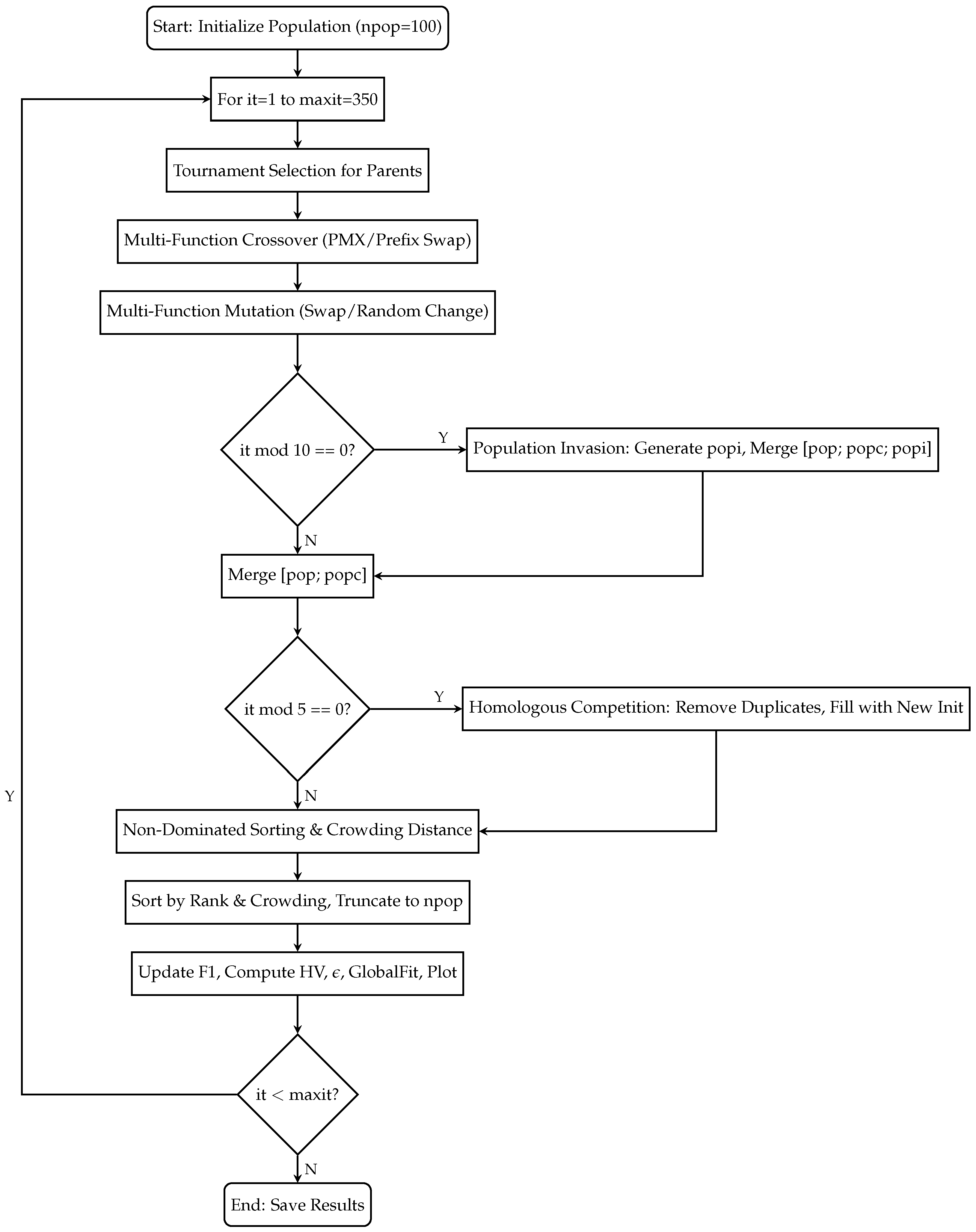
This section presents the Improved Non-dominated Sorting Genetic Algorithm II (I-NSGA-II), which is specifically designed to solve the multimodal hazardous materials transportation optimization model described in Section 2.3. I-NSGA-II extends the standard NSGA-II framework with four key innovations: the population invasion mechanism, homologous competition mechanism, and multi-functional probabilistic crossover and mutation operators. These advancements enhance population diversity, algorithmic convergence, and adaptability to dual-sequence encoding in constrained search spaces. The algorithm flowchart is shown in Figure 2.

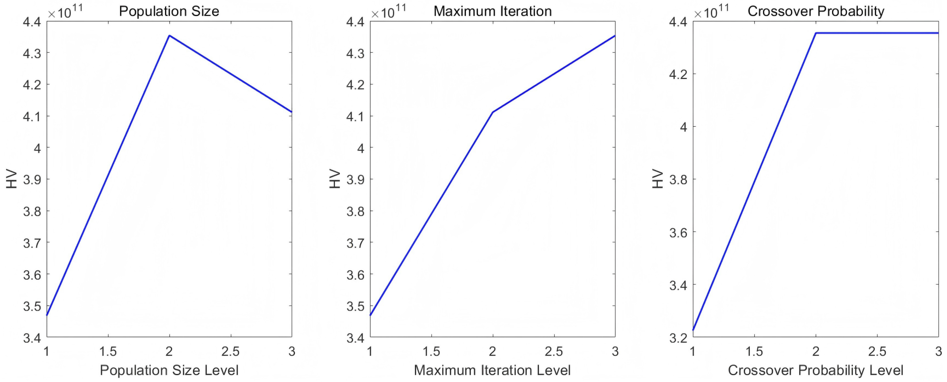
The values npop = 100 and maxit = 350 shown in the flowchart were determined through a prior Taguchi L9 orthogonal experiment (Figure 9), which identified them as the best trade-off between solution quality and computational efficiency. The flowchart of I-NSGA-II is shown in Figure 2. The following steps precisely correspond to the flowchart.

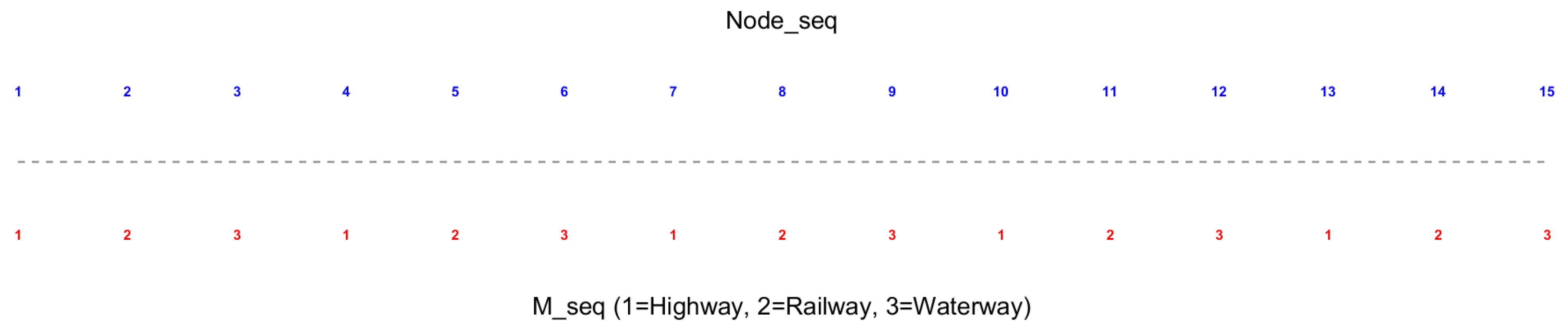
Step 1: Initialize the population of size npop = 100 using dual-sequence encoding ($\mathit{Node}\_\mathit{seq}$ and $\mathit{M}\_\mathit{seq}$). The algorithm begins with population initialization, where each individual is represented using a dual-sequence encoding: When encoding, the node path adopts the node sequence ($\mathit{Node}\_\mathit{seq}$), and the transport mode adopts the M sequence ($\mathit{M}\_\mathit{seq}$). In the initialization stage, the circular structure verifies the path connectivity through the connection diagram matrix and uses the pceFlag indicator to judge the feasibility of the transport mode, so as to effectively prevent the invalid solution from entering the population.

Figure 3 shows the diagram of the coding structure. The $\mathit{Node}\_\mathit{seq}$ marked with blue numbers in the upper row presents the sample path sequence from node 1 to 15, and the $\mathit{M}\_\mathit{seq}$ marked with red numbers in the lower row is assigned the corresponding mode. For easy observation, the gray dotted line separates the sequence. This innovative dual representation supports multimodal constraints. The algorithm handles connections that do not exist under a given mode of transportation in the following ways: in the initialization and crossover/variation stage, the generated node sequence is verified in the connection mapping matrix. If the connection mapping (current node, target node) = 0 under the selected mode of transportation, the individual will be immediately abandoned and replaced by a new effective initialization to ensure the feasibility of 100% of the population.

Step 2: After the population initialization is completed, the fitness evaluation will calculate the three objective values of each individual and impose a penalty function with large constants on the infeasible paths.

Step 3: Next, the non-dominance ranking is the individual distribution level. If the individual p dominates q, then all the objective function values of p are less than or equal to the corresponding values of q, and at least one objective function value is strictly less than q. Within the same level, promote diversity by calculating the crowded distance:

$$d_k^j={\displaystyle \frac{|f_j(k+1)-f_j(k-1)|}{|f_j^{max}-f_j^{min}|}}$$

(16)

In Equation (16), $d_k^j$ represents the crowded distance of individual k on the objective j.

Step 4: After the non-dominant sorting, the tournament selection then selects the parent generation for genetic operations according to the level and crowding distance.

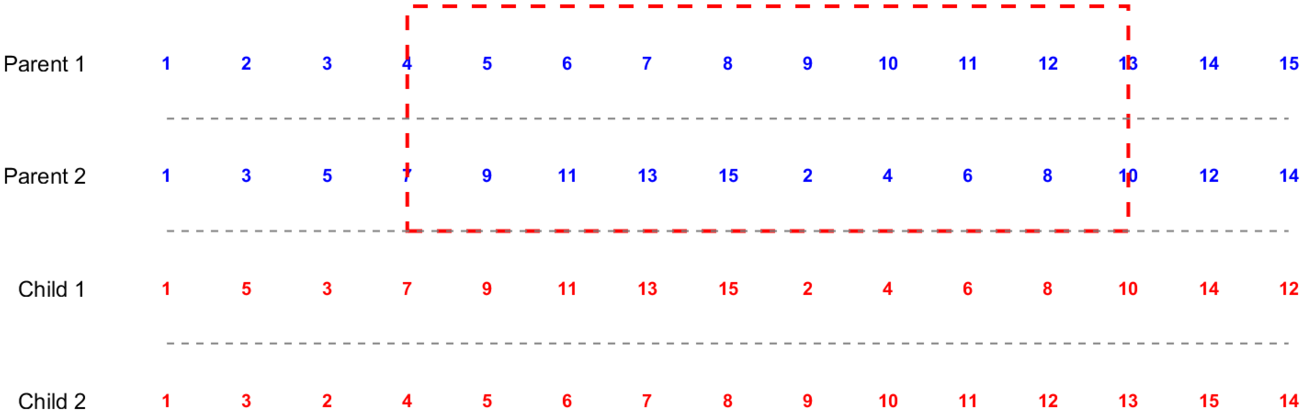
Step 5: Apply the multi-function probabilistic crossover operator. It uses the random value r for probability branching. For example, if $r<0.3$, only partial mapping intersection (PMX) is applied $\mathit{Node}\_\mathit{seq}$ to ensure that no nodes are duplicated; if $0.3<=r<0.6$, then perform a prefix exchange for $\mathit{M}\_\mathit{seq}$ the random index idx; otherwise, perform the above two operations at the same time. This method is different from the traditional uniform crossover. It can adapt to hybrid coding, balance the evolution of paths and patterns, and reduce the generation of invalid offspring. This operator is implemented in MATLAB as CrossoverMulti.m and uses a random value r for probabilistic branching.

Figure 4 shows the PMX cross-operation. The upper two lines show parent generation 1 and parent generation 2, of which the intersection segment is located between points cp1 = 4 and cp2 = 12, and is marked by a red dotted rectangle. The following two lines are shown in the exchange and mapping adjustment to eliminate the duplicated children 1 and children 2. For ease of reading, each line is separated by a gray dotted line to show how the operator maintains the integrity of the path.

Step 6: The mutation mechanism is also innovative and multifunctional. For example, if $r<0.3$, exchange two random positions in $\mathit{Node}\_\mathit{seq}$; if $0.3<=r<0.6$, change the value of the random position in $\mathit{M}\_\mathit{seq}$ to a value between 1 and 3; otherwise, perform two operations at the same time. This directional probability selection mechanism maintains the effectiveness of the solution in the problem of pattern constraints and disabled flags by specifically disturbing the coding components, and its performance is better than the standard variation method. This operator is implemented in MATLAB as MutateMulti.m and uses a random value r to decide whether to swap positions in $\mathit{Node}\_\mathit{seq}$, change values in $\mathit{M}\_\mathit{seq}$, or both.

Figure 5 shows the mutation operation. The figure above shows the original path, and the figure below shows the mutation path after exchanging the 5th and 11th position nodes. The red double arrow marks the exchange operation, and the dotted gray separator is used to distinguish the upper and lower lines to improve visual clarity.

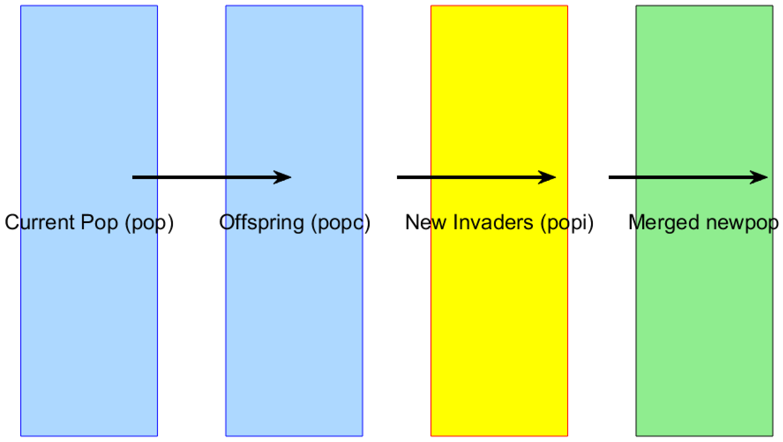
Step 7: After generating offspring popc, the algorithm will merge the population. The innovative population invasion mechanism is triggered every 10 generations (invadeTime = 10) to generate a new population popi and participate in the merger through reinitialization:

$$newpop=[pop;popc;popi]$$

(17)

In the population invasion mechanism, the number of invaders is set to 15% of the current population size. These invaders are newly initialized individuals that are merged into the population every 10 generations to inject fresh genetic material and prevent premature convergence.

Figure 6 shows the population invasion mechanism. The diagram contains three input modules. Among them, the light blue “current population” and “Offspring” represent the existing evolutionary genealogy, and the yellow “new invaders” module emphasizes the external introduction mechanism. The arrow finally converges into the light green “Merge New population” module, which can not only expand the search space but also help the algorithm jump out of the local optimal solution.

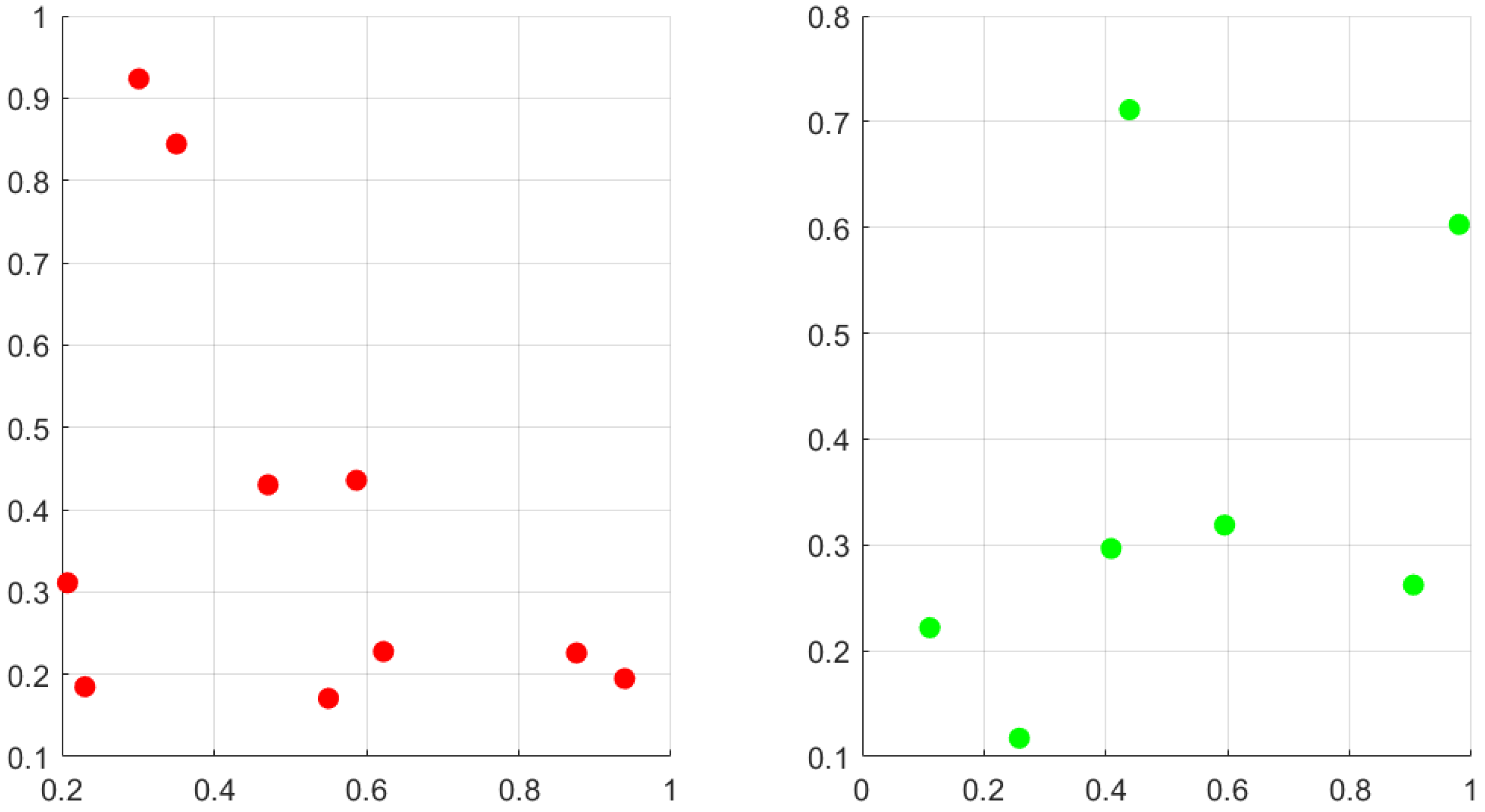
Step 8: After the population invasion mechanism, the innovative homology competition mechanism is activated every five generations on the merged population. It converts the cost matrix into a unique string, as shown in the following equation:

$$\mathrm{str}\_\mathrm{matrix}=\mathrm{strcat}(\mathrm{num}2\mathrm{str}\left(\mathrm{Obj}(:,1)\right),‘\_’,\mathrm{num}2\mathrm{str}\left(\mathrm{Obj}(:,2)\right),‘\_’,\mathrm{num}2\mathrm{str}\left(\mathrm{Obj}(:,3)\right))$$

(18)

The equation uses a unique function to retain the unique index and refill the population with newly initialized individuals. This can eliminate redundancy more effectively than the standard elite retention method and ensure the uniformity of Pareto’s frontier distribution.

Figure 7 shows the homologous competition mechanism. The left sub-chart uses red scatter points to represent a population containing duplicate or similar individuals, simulating the cost points of cluster distribution in the objective space. The sub-chart on the right shows a simplified and diversified collection obtained after repeated individual elimination and supplementation with green dots.

The merged population is then repeated non-dominant sorting and crowding calculations, and then npop individuals are retained through sorting and truncation operations, so as to maintain the elite solution. The iteration process continues to reach the maximum number of iterations maxit, and each iteration will update the Pareto frontier.

Step 9: The performance evaluation indicators are introduced in the following section. The performance evaluation will be measured by the Hypervolume (HV). The following is the calculation equation for Hypervolume (HV):

$$HV=\sum _{n=1}^N\prod _{i=1}^M|P(n,i)-r\left(i\right)|$$

(19)

where P is the Pareto set and $r=[30,{10}^4,5\times {10}^4]$ is the reference point;

$\epsilon$-indicator:

$$\epsilon =max\left(min\left({\displaystyle \frac{Obj}{refPoint}}-idealPoint,\left[\right],1\right)\right)$$

(20)

and Global Fitness (GF):

$$GF=mean\left(\sum {\displaystyle \frac{Obj}{refPoint}},2\right)$$

(21)

with $idealPoint=[0,0,0]$. These indicators are used to track the improvements brought about by innovation.

Pseudocode for I-NSGA-II:

In summary, the I-NSGA-II algorithm realizes the efficient optimization of the multimodal transport path through population invasion mechanism, homology competition mechanism and multi-function probability cross-mutation operators. At the same time, it is superior to the standard NSGA-II algorithm in terms of diversity and convergence. For details of relevant case verification, please refer to Section 4.

Algorithm 1 pseudocode:

Algorithm 1 I-NSGA-II Algorithm

Require:  Network parameters, npop = 100, maxit = 250, pc = 0.8, invadeTime = 10, CompetitionTime = 5 Ensure:  Pareto front F1   1: Initialize pop (dual encoding, ensure valid)   2: Evaluate cost ($f_1,f_2,f_3$)   3: Non-dominated sort and crowding distance   4: for it = 1 to maxit do   5:     Select parents, crossover/mutate to generate popc   6:     if it % invadeTime == 0 then   7:         Generate popi, newpop = [pop; popc; popi]   8:     else   9:         newpop = [pop; popc] 10:     end if 11:     if it % CompetitionTime == 0 then 12:         Remove duplicates, refill newpop 13:     end if 14:     Non-dominated sort, crowding, sort and truncate to pop 15:     Update F1 16:     Compute metrics (HV, $\epsilon$, GF) 17: end for 18: Return F1

3.2. Entropy-Weighted TOPSIS for Optimal Solution Selection

After I-NSGA-II generates the Pareto frontier, EW-TOPSIS processes the adaptation value starting from F1 through the following steps [38,39,40,41]:

1. Duplicate Removal: Form a unique string from the objective and keep different entries through unique.

2. Positivization:

$$X_{up}(:,j)=max\left(fitness(:,j)\right)-fitness(:,j),j=1,2,3.$$

(22)

The equation transforms the original minimization objectives into a maximum form by subtracting each value of the column j from the maximum value of the adaptation matrix. This ensures that all goals can be regarded as “the larger the value, the better” in the next step.

3. Normalization:

$$Z(i,j)={\displaystyle \frac{X_{up}(i,j)-min\left(X_{up}(:,j)\right)}{max\left(X_{up}(:,j)\right)-min\left(X_{up}(:,j)\right)}}.$$

(23)

This equation shows that for each element $(i,j)$, this operation scales the positive value in $X_{up}$ to the [0, 1] interval. The specific method is to subtract the minimum value of column j from the current value and divide it by the extreme difference of column j so as to achieve dimensionless data and ensure that there is comparability between different objectives.

4. Entropy Weighting:

$$p(:,j)={\displaystyle \frac{Z(:,j)}{\sum Z(:,j)}}.$$

(24)

This equation calculates the ratio of each normalized value in column j to the sum of all values in the column, indicating the relative contribution of each solution to the objective function.

$$e_j=-{\displaystyle \frac{\sum p(i,j)·log\left(p\right(i,j\left)\right)}{log\left(m\right)}},$$

(25)

where $log\left(0\right)=0$ is handled specially.

This equation calculates the entropy of the objective j and is used to measure the uncertainty or diversity of the ratio. The summation traverses all the solutions i and normalizes by the logarithm $log\left(m\right)$ based on the number of solutions m, thus limiting the result value to between 0 and 1.

$$D_j=1-e_j.$$

(26)

This equation derives the information utility (or redundancy) of the objective j by subtracting its entropy from 1. Higher utility means stronger distinguishing ability.

$$w_j={\displaystyle \frac{D_j}{\sum D}}.$$

(27)

This equation obtains the weight $w_j$ by normalizing the utility values corresponding to all objectives, ensuring that the sum of these weights is 1, and reflecting its relative importance based on the information entropy.

5. Distance and Scoring:

The definition of the positive ideal solution (PIS) is as follows:

$$max\left(Z\right(:,j\left)\right)\mathrm{for}\mathrm{each}j.$$

(28)

This equation represents the best value that each normalized objective j can reach in all solutions.

The definition of negative ideal solution (NIS) is as follows:

$$min\left(Z\right(:,j\left)\right)\mathrm{for}\mathrm{each}j.$$

(29)

This equation represents the minimum possible value of each normalized objective j in all solutions.

$$D_P\left(i\right)=\sqrt{\sum _j{w}_j{(Z(i,j)-max\left(Z(:,j)\right))}^2}.$$

(30)

The equation calculates the weighted Euclidean distance from the solution i to the positive ideal solution (PIS), in which the deviation of the objective j is squared, weighted by $w_j$, summed, and then takes the square root.

$$D_N\left(i\right)=\sqrt{\sum _j{w}_j{(Z(i,j)-min\left(Z(:,j)\right))}^2}.$$

(31)

The equation calculates the weighted Euclidean distance from the solution i to the negative ideal solution (NIS), whose structure is similar to $D_P\left(i\right)$.

$$S\left(i\right)={\displaystyle \frac{D_N\left(i\right)}{D_P\left(i\right)+D_N\left(i\right)}}.$$

(32)

This calculates the relative closeness score for solution i, ranging from 0 to 1, where higher values indicate closer proximity to the PIS and farther from the NIS.

$$stan{d}_S\left(i\right)={\displaystyle \frac{S\left(i\right)}{\sum S}}.$$

(33)

This normalizes the closeness scores across all solutions so they sum to 1, facilitating ranking and selection as probabilities or relative preferences.

The above is the pseudocode of Algorithm 2.

Algorithm 2 EW-TOPSIS

Require: Input: Pareto front F1 Ensure: Output: Optimal result     Extract fitness from F1     Remove duplicates     Positivize: $X_{up}=\mathrm{Min}2\mathrm{Max}\left(fitness\right)$     Normalize to Z     Compute $w=\mathrm{Entropy}\_\mathrm{Method}(Z)$     Compute $D_P,D_N$     Compute $S,stan{d}_S$     Select top by $stan{d}_S$: $result=fitness(top,:)$

4. Case Study

4.1. Case Description

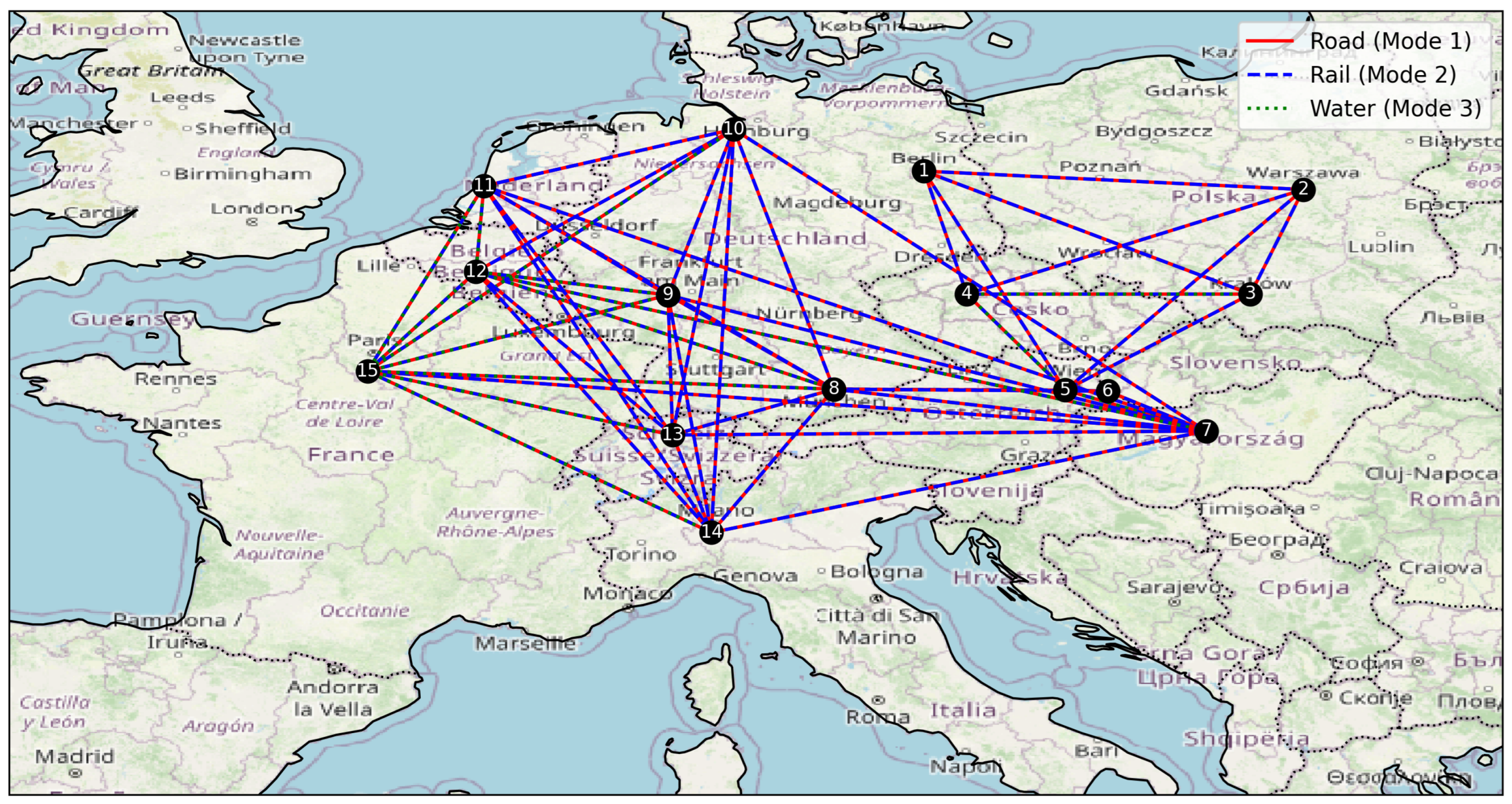
To evaluate the performance of the proposed improved NSGA-II algorithm, a case study is conducted on a hazardous materials transportation network in Europe. This network models multimodal transportation routes from Berlin to Paris, incorporating road, rail, and water modes. The research motivation of this case comes from the expanding scale of hazardous materials logistics in Europe. As revealed by many recent transportation accident research institutes, safety, cost-effectiveness, and environmental impact have become key factors that need to be considered urgently in the industry.

This route was selected because it represents one of Europe’s major hazardous materials corridors, with an annual transport volume exceeding 100,000 tons. It connects key industrial centers while crossing multiple countries under EU regulations, providing an ideal testbed for evaluating multimodal optimization under international constraints.

The network contains 15 nodes, representing the main cities that take on different functions in the transportation link.

Table 2. Node information.

Number	City Name	Full Name	Type	Description
1	Berlin	Berlin, Germany	Start	Main hazardous materials export center
2	Warsaw	Warsaw, Poland	Intermediate
3	Krakow	Krakow, Poland	Intermediate
4	Prague	Prague, Czech Republic	Intermediate
5	Vienna	Vienna, Austria	Intermediate
6	Bratislava	Bratislava, Slovakia	Intermediate
7	Budapest	Budapest, Hungary	Intermediate
8	Munich	Munich, Germany	Intermediate
9	Frankfurt	Frankfurt, Germany	Intermediate
10	Hamburg	Hamburg, Germany	Intermediate
11	Amsterdam	Amsterdam, Netherlands	Intermediate
12	Brussels	Brussels, Belgium	Intermediate
13	Zurich	Zurich, Switzerland	Intermediate
14	Milan	Milan, Italy	Intermediate
15	Paris	Paris, France	End	Import endpoint with strict emission regulations

lists the details of the node, including the number, the city name, and its function description. Berlin is the main export hub of hazardous materials, and Paris serves as an import terminal that needs to comply with strict emission regulations. The intermediate node provides transshipment and route allocation support.

The global parameters in the model are summarized in

Table 3. Global parameters.

Parameter	Value
Q (Total Transportation Volume)	100
$s_k$ (Severity Score)	5
${\mathrm{ins}}_k$ (Unit Insurance Cost)	0.10
$C^m$ (Mode Capacity Limits: Road, Rail, Water)	[500, 1000, 2000]
$s^m$ (Mode Speeds km/h: Road, Rail, Water)	[80, 60, 40]
${\mathrm{TW}}_{max},{\mathrm{TW}}_{min}$ (Time Window in Hours)	0, 48

. These parameters include total transportation volume, severity score, unit insurance cost, carrying capacity, speed, and time window constraints of highway, railway, and waterway transportation mode [42].

The network edges connect these nodes, with attributes such as distance, ban flags, and mode-specific parameters. There are 52 valid edges, excluding empty rows in the data. The

Table 4. Edge data.

Edge (u → v)	d	Ban	Mode 1 (p, c, e)	Mode 2 (p, c, e)	Mode 3 (p, c, e)
1 → 2	519.0	0.0	0.00000519, 1.038, 0.02595	0.000003115, 0.2078, 0.01038	-
1 → 3	595.0	0.0	0.00000595, 1.19, 0.02975	0.00000357, 0.238, 0.0119	-
1 → 4	350.0	0.0	0.0000035, 0.7, 0.0175	0.0000021, 0.14, 0.007	-
1 → 5	680.0	0.0	0.0000068, 1.36, 0.034	0.00000408, 0.272, 0.0136	-
2 → 3	297.0	0.0	0.00000297, 0.594, 0.01485	0.000001782, 0.1188, 0.00594	-
2 → 4	679.0	0.0	0.00000679, 1.358, 0.03395	0.000004074, 0.2716, 0.01358	-
2 → 5	1136.0	0.0	0.00001136, 2.272, 0.0568	0.000006816, 0.4544, 0.02272	-
3 → 4	539.0	0.0	0.00000539, 1.078, 0.02695	0.000003234, 0.2156, 0.01078	0.000002695, 0.1078, 0.00539
3 → 5	839.0	0.0	0.00000839, 1.678, 0.04195	0.000005034, 0.3356, 0.01678	-
4 → 5	300.0	0.0	0.000003, 0.6, 0.015	0.0000018, 0.12, 0.006	0.0000015, 0.06, 0.003
5 → 6	80.0	0.0	0.0000008, 0.16, 0.004	0.00000048, 0.032, 0.0016	-
5 → 7	243.0	0.0	0.00000243, 0.486, 0.01215	0.000001458, 0.0972, 0.00486	0.000001215, 0.0486, 0.00243
5 → 8	436.0	0.0	0.00000436, 0.872, 0.0218	0.000002616, 0.1744, 0.00872	-
6 → 7	201.0	0.0	0.00000201, 0.402, 0.01005	0.000001206, 0.0804, 0.00402	-
6 → 8	461.0	0.0	0.00000461, 0.922, 0.02305	0.000002766, 0.1844, 0.00922	-
7 → 8	685.0	0.0	0.00000685, 1.37, 0.03425	0.00000411, 0.274, 0.0137	-
7 → 9	964.0	0.0	0.00000964, 1.928, 0.0482	0.000005784, 0.3856, 0.01928	-
7 → 10	1166.0	0.0	0.00001166, 2.332, 0.0583	0.000006996, 0.4664, 0.02332	-
7 → 11	1396.0	0.0	0.00001396, 2.792, 0.0698	0.000008376, 0.5584, 0.02792	-
7 → 12	1354.0	0.0	0.00001354, 2.708, 0.0677	0.000008124, 0.5416, 0.02708	0.00000677, 0.2708, 0.01354
7 → 13	997.0	0.0	0.00000997, 1.994, 0.04985	0.000005982, 0.3988, 0.01994	-
7 → 14	958.0	0.0	0.00000958, 1.916, 0.0479	0.000005748, 0.3832, 0.01916	-
7 → 15	1486.0	0.0	0.00001486, 2.972, 0.0743	0.000008916, 0.5944, 0.02972	-
8 → 9	391.0	0.0	0.00000391, 0.782, 0.01955	0.000002346, 0.1564, 0.00782	-
8 → 10	791.0	0.0	0.00000791, 1.582, 0.03955	0.000004746, 0.3164, 0.01582	-
8 → 11	826.0	0.0	0.00000826, 1.652, 0.0413	0.000004956, 0.3304, 0.01652	-
8 → 12	784.0	0.0	0.00000784, 1.568, 0.0392	0.000004704, 0.3136, 0.01568	0.00000392, 0.1568, 0.00784
8 → 13	314.0	0.0	0.00000314, 0.628, 0.0157	0.000001884, 0.1256, 0.00628	-
8 → 14	493.0	0.0	0.00000493, 0.986, 0.02465	0.000002958, 0.1972, 0.00986	-
8 → 15	828.0	0.0	0.00000828, 1.656, 0.0414	0.000004968, 0.3312, 0.01656	0.00000414, 0.1656, 0.00828
9 → 10	508.0	0.0	0.0000414289, 1.51, 0.46	0.00000508, 1.016, 0.0254	-
9 → 11	440.0	0.0	0.0000044, 0.88, 0.022	0.00000264, 0.176, 0.0088	-
9 → 12	382.0	0.0	0.00000382, 0.764, 0.0191	0.000002292, 0.1528, 0.00764	0.00000191, 0.0764, 0.00382
9 → 13	409.0	0.0	0.00000409, 0.818, 0.02045	0.000002454, 0.1636, 0.00818	-
9 → 14	646.0	0.0	0.00000646, 1.292, 0.0323	0.000003876, 0.2584, 0.01292	-
9 → 15	571.0	0.0	0.00000571, 1.142, 0.02855	0.000003426, 0.2284, 0.01142	0.000002855, 0.1142, 0.00571
10 → 11	486.0	0.0	0.00000486, 0.972, 0.0243	0.000002916, 0.1944, 0.00972	-
10 → 12	602.0	0.0	0.00000602, 1.204, 0.0301	0.000003612, 0.2408, 0.01204	-
10 → 13	857.0	0.0	0.00000857, 1.714, 0.04285	0.000005142, 0.3428, 0.01714	-
10 → 14	1108.0	0.0	0.00001108, 2.216, 0.0554	0.000006648, 0.4432, 0.02216	-
10 → 15	894.0	0.0	0.00000894, 1.788, 0.0447	0.000005364, 0.3576, 0.01788	0.00000447, 0.1788, 0.00894
11 → 12	204.0	0.0	0.00000204, 0.408, 0.0102	0.000001224, 0.0816, 0.00408	0.00000102, 0.0408, 0.00204
11 → 13	836.0	0.0	0.00000836, 1.672, 0.0418	0.000005016, 0.3344, 0.01672	-
11 → 14	1075.0	0.0	0.00001075, 2.15, 0.05375	0.00000645, 0.43, 0.0215	-
11 → 15	504.0	0.0	0.00000504, 1.008, 0.0252	0.000003024, 0.2016, 0.01008	0.00000252, 0.1008, 0.00504
12 → 13	653.0	0.0	0.00000653, 1.306, 0.03265	0.000003918, 0.2612, 0.01306	-
12 → 14	893.0	0.0	0.00000893, 1.786, 0.04465	0.000005358, 0.3572, 0.01786	-
12 → 15	304.0	0.0	0.00000304, 0.608, 0.0152	0.000001824, 0.1216, 0.00608	0.00000152, 0.0608, 0.00304
13 → 14	279.0	0.0	0.00000279, 0.558, 0.01395	0.000001674, 0.1116, 0.00558	-
13 → 15	653.0	0.0	0.00000653, 1.306, 0.03265	0.000003918, 0.2612, 0.01306	0.000003265, 0.1306, 0.00653
14 → 15	849.0	0.0	0.00000849, 1.698, 0.04245	0.000005094, 0.3396, 0.01698	0.000004245, 0.1698, 0.00849

provides the edge data to illustrate the structure [43].

Transshipment data at each node specifies mode conversion costs and probabilities for switches between modes (1: road, 2: rail, 3: water).

Table 5. Transshipment data.

Node	From 1 to 2 (p, c, e)	From 1 to 3 (p, c, e)	From 2 to 1 (p, c, e)	From 2 to 3 (p, c, e)	From 3 to 1 (p, c, e)	From 3 to 2 (p, c, e)
1	0.000946, 48.16, 0.92	0.000433, 10.62, 0.94	0.000485, 48.67, 0.97	0.000868, 21.78, 0.45	0.000866, 22.68, 0.25	0.000601, 47.45, 0.73
2	0.000123, 48.51, 0.85	0.000726, 26.36, 0.26	0.000719, 37.78, 0.44	0.000697, 44.42, 0.32	0.000959, 39.52, 0.60	0.000651, 26.78, 0.32
3	0.000420, 40.31, 0.11	0.000204, 11.84, 0.14	0.000870, 38.15, 0.53	0.000188, 29.66, 0.53	0.000256, 27.35, 0.46	0.000654, 35.40, 0.14
4	0.000613, 13.89, 0.65	0.000991, 15.60, 0.57	0.000890, 39.63, 0.73	0.000732, 24.38, 0.36	0.000828, 42.40, 0.88	0.000922, 30.45, 0.55
5	0.000818, 36.00, 0.73	0.000816, 45.60, 0.40	0.000438, 13.76, 0.62	0.000132, 28.62, 0.59	0.000358, 33.63, 0.13	0.000134, 42.90, 0.42
6	0.000437, 35.03, 0.55	0.000871, 36.35, 0.25	0.000164, 35.70, 0.12	0.000627, 47.61, 0.62	0.000449, 35.73, 0.51	0.000591, 47.66, 0.45
7	0.000214, 30.89, 0.79	0.000294, 34.92, 0.18	0.000147, 31.25, 0.59	0.000674, 39.04, 0.98	0.000565, 22.92, 0.82	0.000344, 27.56, 0.17
8	0.000965, 46.21, 0.28	0.000162, 14.03, 0.12	0.000185, 37.32, 0.16	0.000387, 43.80, 0.12	0.000833, 21.27, 0.21	0.000727, 35.16, 0.89
9	0.000812, 41.58, 0.18	0.000545, 12.30, 0.59	0.000497, 45.51, 0.42	0.000205, 15.72, 0.79	0.000656, 14.04, 0.18	0.000731, 12.91, 0.84
10	0.000350, 17.52, 0.52	0.000418, 33.35, 0.17	0.000977, 49.45, 0.73	0.000582, 22.38, 0.83	0.000716, 16.50, 0.92	0.000840, 47.99, 0.75
11	0.000736, 13.25, 0.18	0.000988, 24.97, 0.43	0.000832, 47.89, 0.99	0.000778, 25.05, 0.18	0.000799, 32.34, 0.48	0.000916, 14.45, 0.54
12	0.000110, 28.75, 0.15	0.000207, 14.70, 0.68	0.000771, 33.33, 0.97	0.000437, 21.43, 0.88	0.000301, 48.53, 0.11	0.000973, 11.73, 0.90
13	0.000762, 42.14, 0.35	0.000260, 40.02, 0.83	0.000991, 26.50, 0.43	0.000799, 23.63, 0.94	0.000873, 27.16, 0.78	0.000779, 14.12, 0.91
14	0.000555, 43.06, 0.39	0.000906, 25.57, 0.11	0.000915, 13.65, 0.39	0.000955, 48.02, 0.62	0.000669, 27.94, 0.36	0.000396, 36.90, 0.78
15	0.000575, 49.72, 0.17	0.000598, 48.77, 0.57	0.000666, 37.83, 0.51	0.000665, 33.37, 0.91	0.000141, 21.24, 0.96	0.000901, 28.23, 0.66

presents transshipment data for selected nodes [44].

The multimodal transportation network in the present case is illustrated in Figure 8.

4.2. Case Solution

The improved NSGA-II algorithm introduced in this work was implemented using MATLAB R2024b and underwent performance evaluation on a Windows 11 system configured with a 2.30 GHz CPU and 16 GB RAM.

In order to determine the optimal parameter combination of the I-NSGA-II algorithm, this study used Taguchi experimental design and an L9 orthogonal table for analysis. Select the three key parameters of population size (level: 50, 100, 150), the maximum number of iterations (level: 150, 250, 350), and cross probability (level: 0.6, 0.8, 1.0), and take the hypervolume (HV) as the main response indicator. The main effect Figure 9 shows that the average HV value corresponding to the second level of population size is the highest; the third level of the maximum number of iterations makes HV continue to increase. The second level of cross-probability is insensitive to further increased performance while achieving the best performance.

Figure 9. Main effects plot on HV (Taguchi experiment).

Figure 9. Main effects plot on HV (Taguchi experiment).

The results show that a larger population size and more iterations can improve the quality and convergence of the solution, which is consistent with the basic principle of evolutionary algorithms. Thus, the improved NSGA-II algorithm was implemented with a population size of 100, maximum iterations of 350, crossover probability of 0.8 [45], and reference point [30, ${10}^4$, $5\times {10}^4$] [46]. The relevant parameters were configured in accordance with the cited references above. The experiment involved 30 independent runs to ensure statistical reliability.

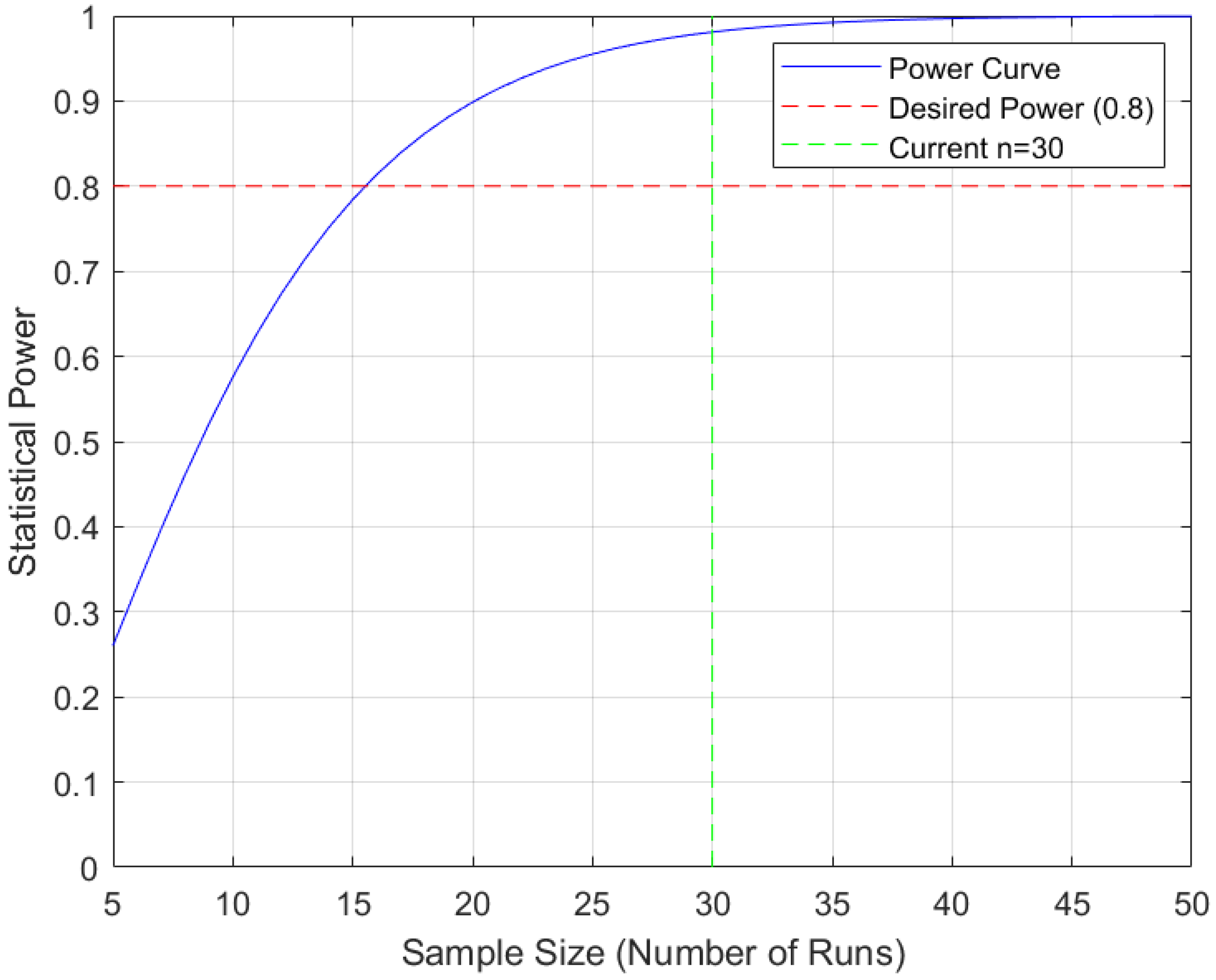
To assess the statistical robustness of the results, a power analysis was performed, yielding an effect size of 0.7628 and a power of 0.9810 for 30 runs [47]. This high power value, exceeding the conventional threshold of 0.8, confirms that the sample size is sufficient to detect meaningful differences with low risk of Type II errors. The computational efficiency is evidenced by an average runtime of 143.6015 s per run, with a standard deviation of 37.9684 seconds, indicating consistent performance across executions. Figure 10 illustrates the power curve derived from 30 experimental runs.

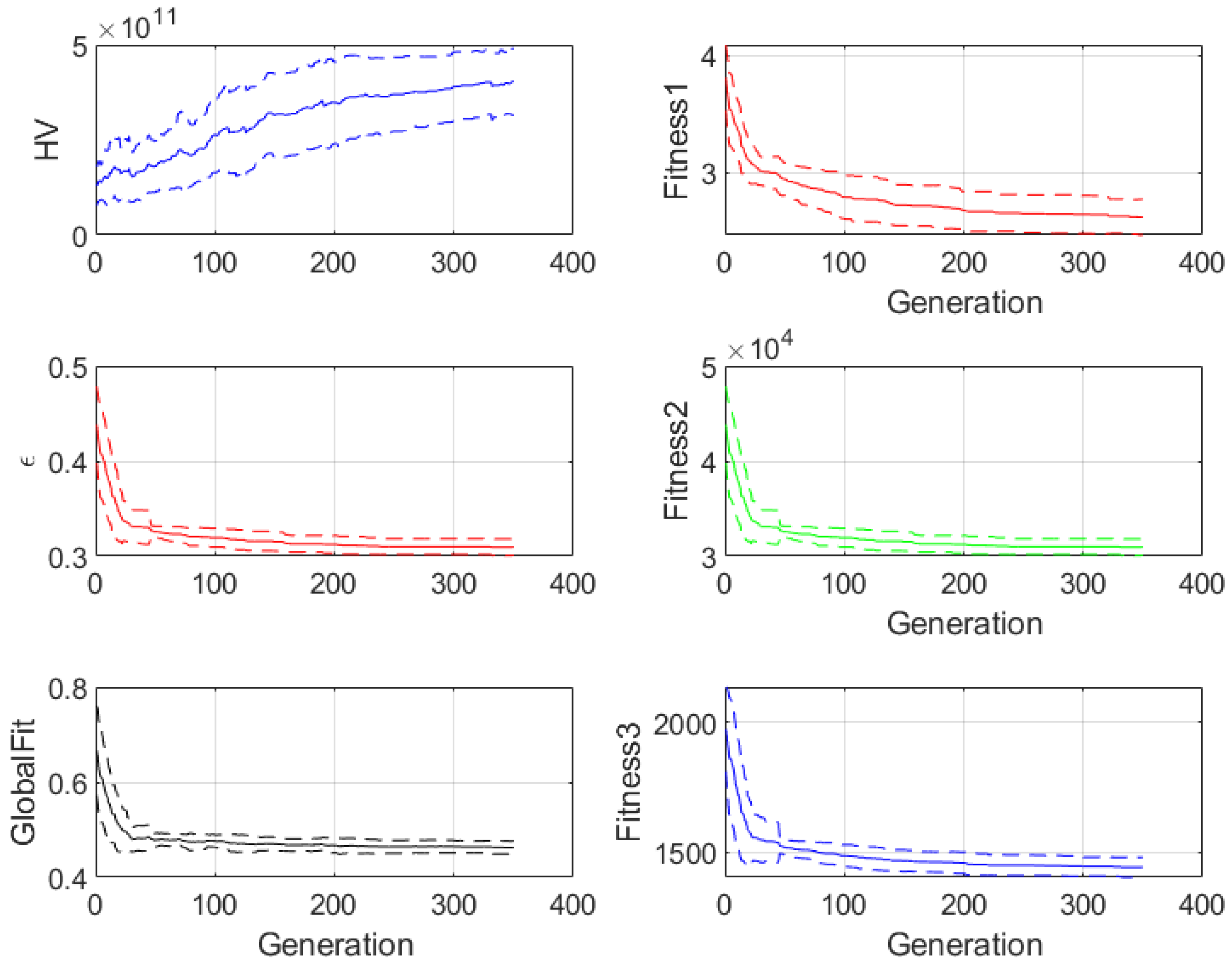
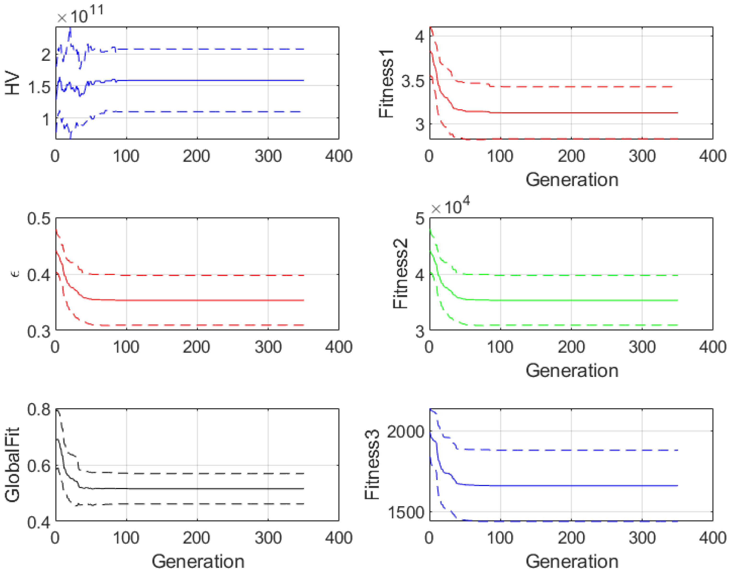
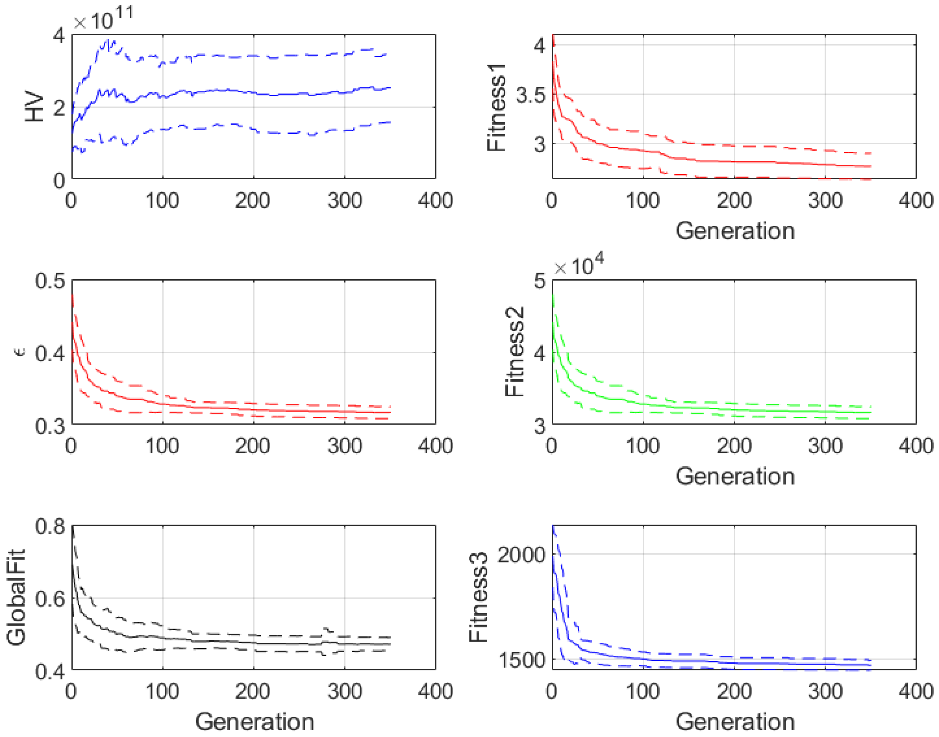
A comparison with the baseline NSGA-II and MOQPSO, executed under identical conditions, reveals the superiority of the improved variant. As shown in

Table 6. Comparison with baseline NSGA-II and MOQPSO.

Metric	Improved Mean	Baseline Mean	MOQPSO Mean
HV	$3.6997\times {10}^{11}$	$1.5857\times {10}^{11}$	$2.3292\times {10}^{11}$
$\epsilon$	0.3101	0.3534	0.3282
GF	0.4642	0.5153	0.4880

and Figure 11, Figure 12 and Figure 13, the improved algorithm achieves a mean hypervolume (HV) of $3.6997\times {10}^{11}$ (standard deviation $9.7008\times {10}^{10}$), representing a 133% improvement over the baseline’s $1.5857\times {10}^{11}$ and a 58.8% improvement over MOQPSO’s $2.3292\times {10}^{11}$. Similarly, the epsilon indicator ($\epsilon$) is reduced by 12% to 0.3101 (standard deviation 0.0082) from the baseline’s 0.3534 and by 5.5% from MOQPSO’s 0.3282. The global fit (GF) is reduced by 10% to 0.4642 (standard deviation 0.0136) from the baseline’s 0.5153 and by 4.9% from MOQPSO’s 0.4880. These enhancements underscore the effectiveness of the incorporated population invasion and homologous competition mechanisms in generating more diverse and higher-quality Pareto fronts.

Following the comprehensive comparison with the baseline NSGA-II and MOQPSO under identical conditions, the I-NSGA-II algorithm was applied to solve the multi-objective route planning problem. After parameter tuning, the algorithm generated a Pareto front consisting of four non-dominated solutions, as detailed in

Table 7. Pareto front solutions.

Solution	Risk	Cost	Emission	Path Nodes	Transportation Modes
1	2.3815	$3.1763\times {10}^4$	$1.588\times {10}^3$	1-4-5-8-9-12-15	2-2-2-2-2-2
2	2.6283	$2.9434\times {10}^4$	$1.385\times {10}^3$	1-4-5-8-9-12-15	2-2-2-2-3-3
3	3.3428	$3.2490\times {10}^4$	$1.372\times {10}^3$	1-4-5-8-9-12-15	2-3-2-2-3-3
4	2.4012	$3.2776\times {10}^4$	$1.554\times {10}^3$	1-4-5-8-9-12-15	2-2-2-2-2-3

. Although the number of unique solutions remains limited due to stringent constraints (time windows, mode compatibility, and regulatory bans), the Spread metric reached 0.87, indicating satisfactory uniformity and diversity of the Pareto front.

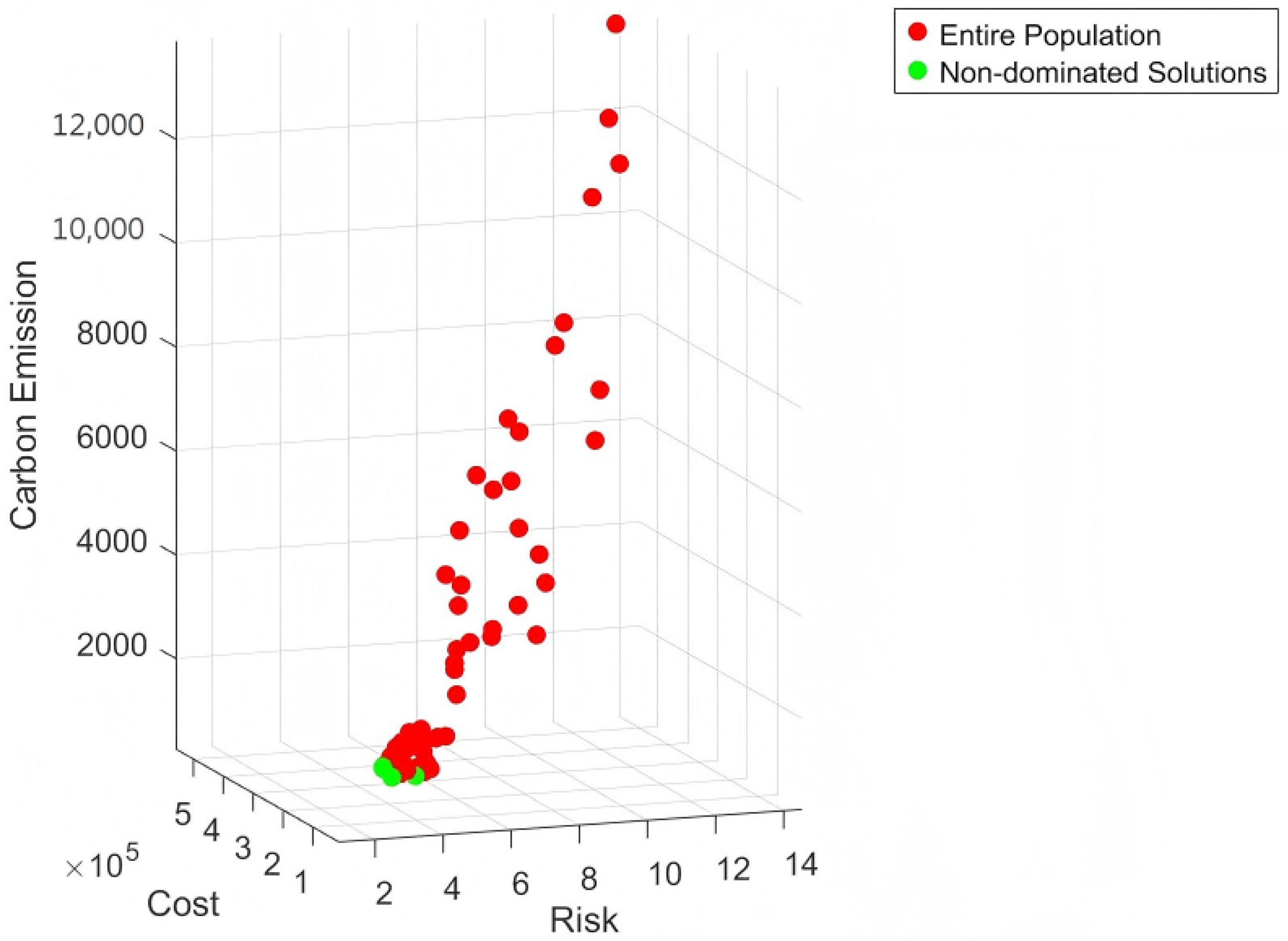
All solutions converge on the path 1-4-5-8-9-12-15, with variations primarily in rail (mode 2) and water (mode 3) selections, reflecting trade-offs between low risk and minimized cost and emission. For instance, Solution 2 offers the lowest cost ($2.9434\times {10}^4$) and emission ($1.385\times {10}^3$) at a slightly higher risk (2.6283), while Solution 1 prioritizes minimal risk (2.3815). The three-dimensional representation in Figure 14 illustrates the front’s spread, confirming balanced optimization across objectives.

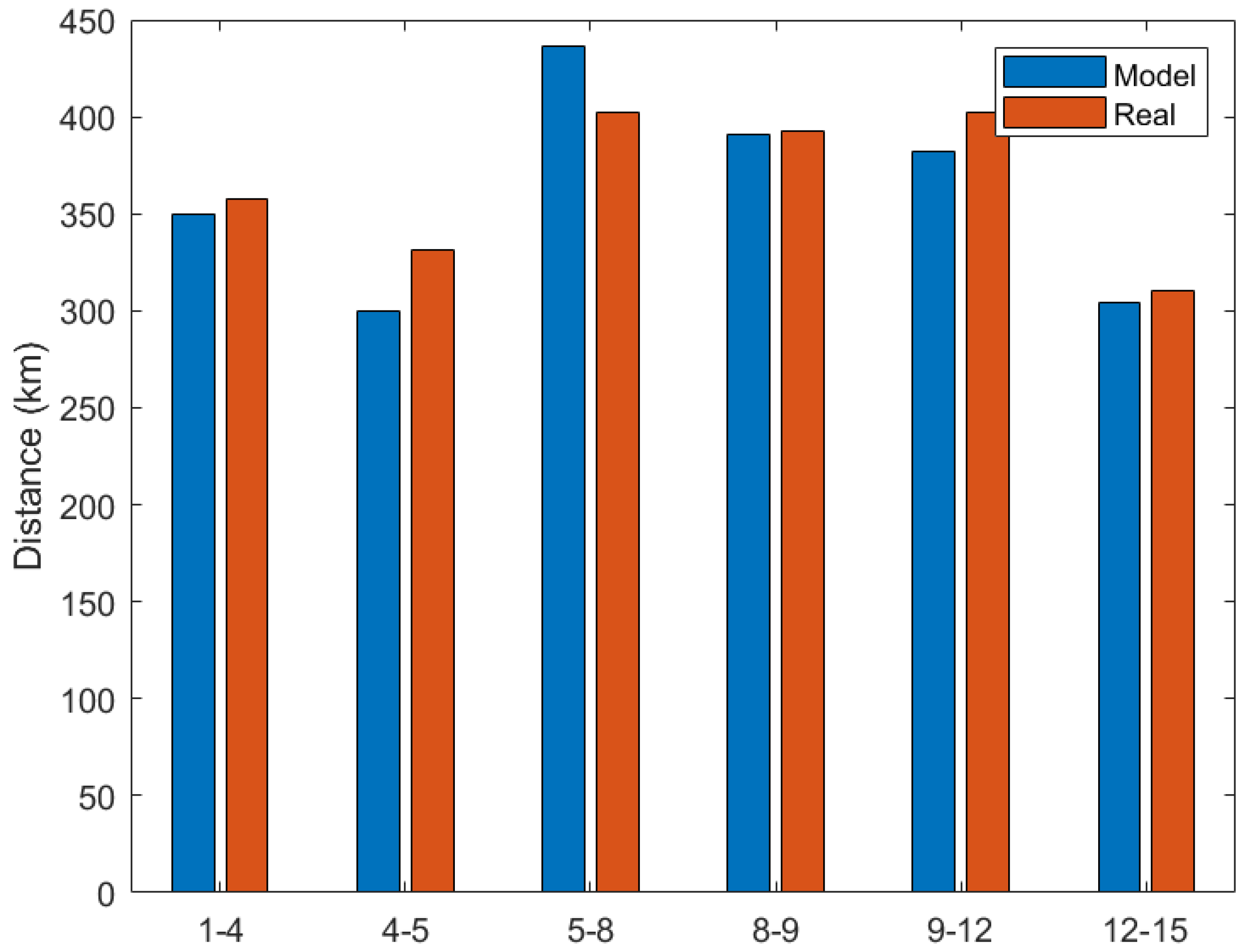
To validate the model’s fidelity to real-world conditions, the paths derived from the Pareto front were compared against actual distances retrieved from Google Maps 25.25.3. This comparison produced the edge error data reported in

Table 8. Real-world validation errors.

Edge	Error (Model − Real, km)
1–4	−8
4–5	−31
5–8	34
8–9	−2
9–12	−20
12–15	−6
Overall RMSE	20.9006

, with an overall root mean square error of 20.9006 km.

These findings affirm the network’s accurate representation of geographical realities. The corresponding bar chart visualization is presented in Figure 15.

To select the optimal solution from the Pareto front obtained via the improved NSGA-II algorithm, the Entropy Weight Technique for Order Preference by Similarity to Ideal Solution (EW-TOPSIS) method is employed. This approach objectively determines weights based on the information entropy of the objective values and ranks the solutions by their closeness to the ideal point, ensuring a balanced compromise among risk, cost, and emission objectives.

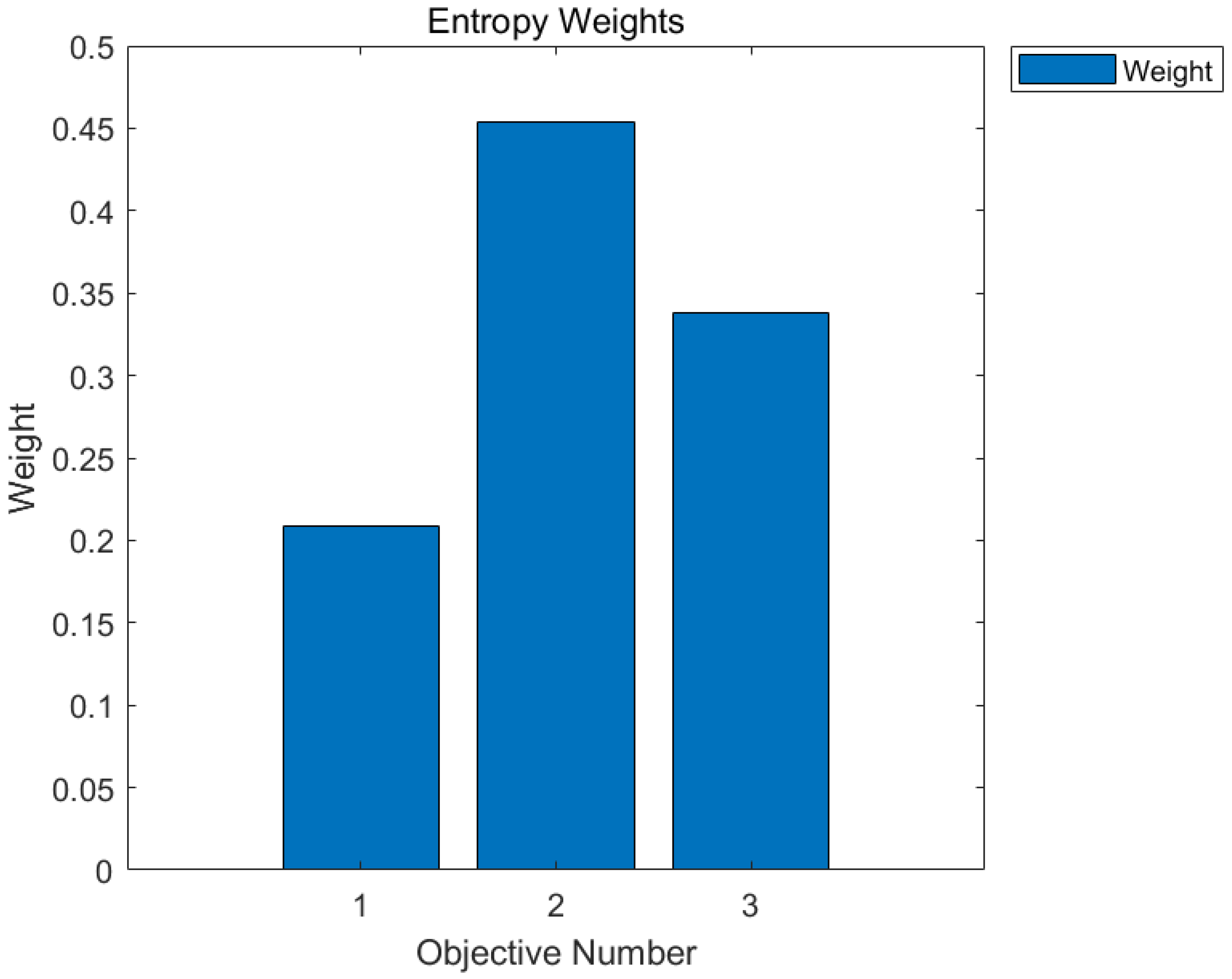
The entropy values were computed using Equation (25), based on the variability of the normalized Pareto solutions. The entropy weights for the three objectives are calculated as follows: risk (0.2082), cost (0.4538), and emission (0.3380). These weights reflect the relative importance derived from the variability in the Pareto solutions, with cost exhibiting the highest entropy-based utility. The weight distribution is illustrated in Figure 16.

Figure 16 shows that the higher the weight, the greater the variability of that objective in the Pareto front.

The normalized TOPSIS scores for the four unique Pareto solutions are presented in

Table 9. Normalized scores and objective values matrix (sorted by score).

Scheme	Normalized Score	Risk	Cost	Emission
2	0.4268	2.6283	29,434	1385.3
3	0.2089	3.3428	32,490	1372.3
1	0.1936	2.3815	31,763	1587.6
4	0.1707	2.4012	32,776	1554.2

, sorted in descending order.

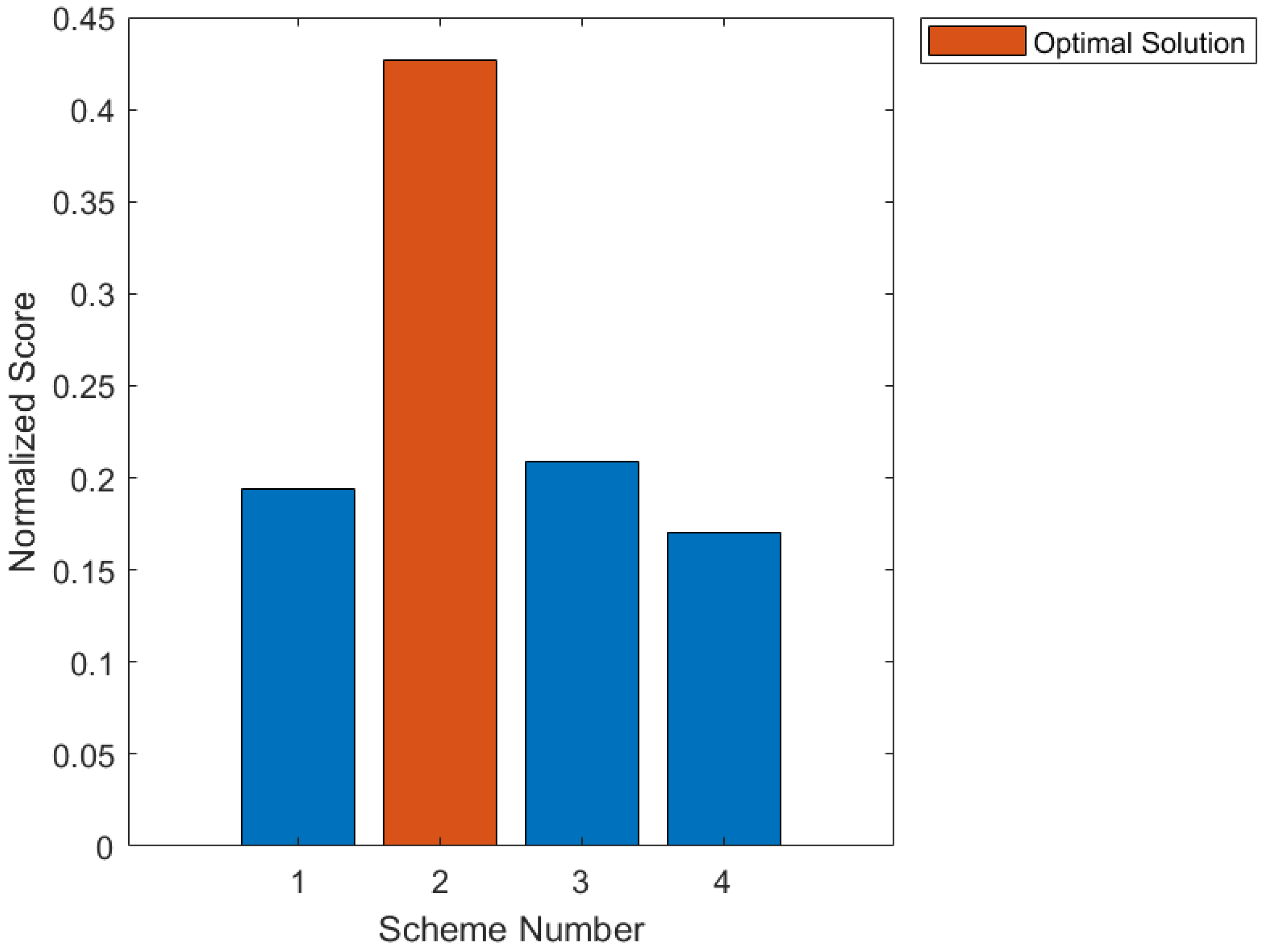
The matrix includes scheme numbers, scores, and corresponding objective values. Scheme 2 achieves the highest score of 0.4268, indicating its superior overall performance. The scores are visualized in Figure 17, where the optimal scheme is highlighted.

The optimal solution yields the following objective values: risk = 2.6283, cost = 29,434, emission = 1385.3. The associated effective path nodes are [1, 4, 5, 8, 9, 12, 15], with transportation modes [2, 2, 2, 2, 3, 3]. This solution demonstrates an effective trade-off, minimizing cost while maintaining acceptable risk and emission levels.

In order to further verify the robustness of the decision-making process, this study compares the entropy power method and the manual empowerment method (setting the risk, cost, and emission weights to 0.4, 0.3, and 0.3, respectively). As shown in

Table 10. Comparison of route ranking between entropy-weighted TOPSIS and manual weighting.

Scheme	Entropy Rank	Manual Rank	Risk	Cost	Emission
1	3	2	2.3815	31,763	1587.6
2	1	1	2.6283	29,434	1385.3
3	2	4	3.3428	32,490	1372.3
4	4	3	2.4012	32,776	1554.2

Note: Both methods consistently select Scheme 2 as the optimal solution (lowest cost with acceptable risk and emission). Manual weights used: risk 0.4, cost 0.3, emission 0.3. Entropy weights: risk 0.2082, cost 0.4538, emission 0.3380.

, the sorting results of the entropy weighting method are: Scheme 2 > Scheme 3 > Scheme 1 > Scheme 4; the sorting results of the manual empowerment method are: Scheme 2 > Scheme 1 > Scheme 4 > Scheme 3. It is worth noting that both methods unanimously determine that Scheme 2 is the optimal path (risk = 2.6283, cost = 29,434, emission = 1385.3, corresponding path 1-4-5-8-9-12-15, and transportation mode 2-2-2-2-3-3). This consistency shows that the TOPSIS method based on the entropy weight method not only provides objective prioritization but also is highly consistent with the subjective judgment of experts, thus enhancing the reliability of the selected transportation scheme.

This EW-TOPSIS integration provides a robust decision-making framework, confirming the efficacy of the proposed algorithm in real-world chemical transportation scenarios.

4.3. Sensitivity Analysis

In order to evaluate the impact of changes in the key parameter transportation volume Q, risk severity score $s_k$, and transportation mode capacity factor $C^m$ on the average risk, cost, and emission objective, we conducted a sensitivity analysis. The evaluation not only reveals the robustness of the model but also identifies the core parameters that have a significant impact on the optimization results.

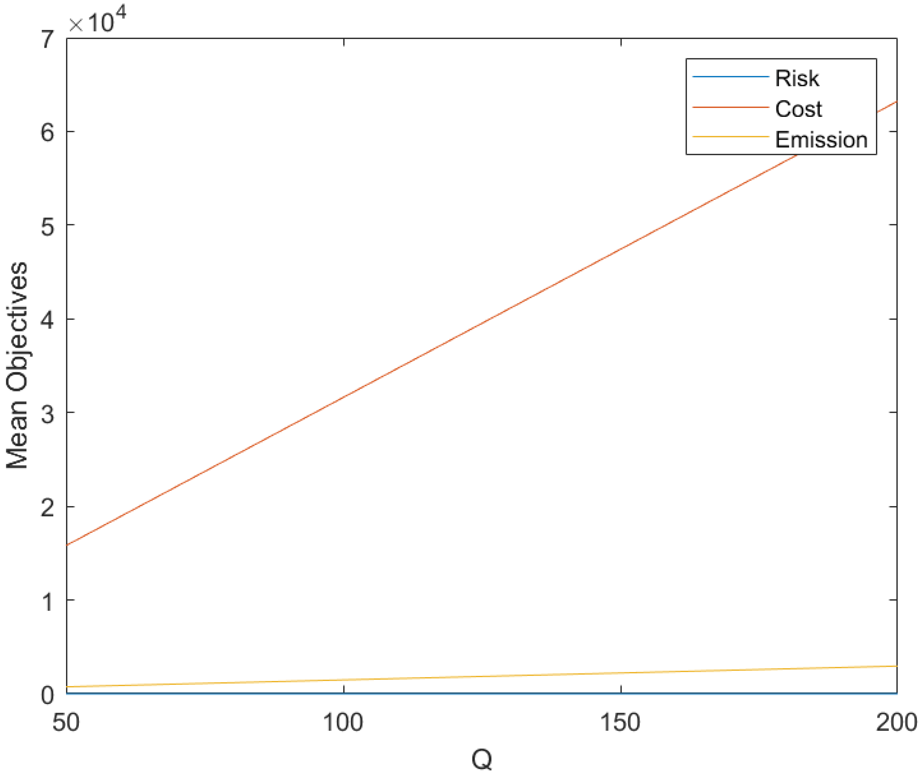
In the study of Q (test values are 50, 100, 150, and 200, respectively),

Table 11. Sensitivity for Q.

Q	Risk	Cost	Emission
50	1.3442	15,807.85	737.43
100	2.6884	31,615.70	1474.86
150	4.0327	47,423.55	2212.29
200	5.3769	63,231.40	2949.72

and Figure 18 show that with the increase of Q, costs and emissions are on a linear upward trend, while the risk value is guaranteed to remain stable. This phenomenon is consistent with the design logic of the objective function: in the calculation of cost and emission, Q participates in the operation as a direct multiplier, resulting in the proportional growth of the two with Q. Specifically, when Q increased from 100 times to 200 times, the cost (from 31,615.70 to 63,231.40) and emissions (from 1474.86 to 2949.72) almost doubled, reflecting that larger-scale operation will simultaneously push up resource demand and environmental load. The insensitivity of the risk value to the change of Q shows that in this model, the risk mainly depends on the characteristics of the transport path, rather than increasing with the expansion of the volume.

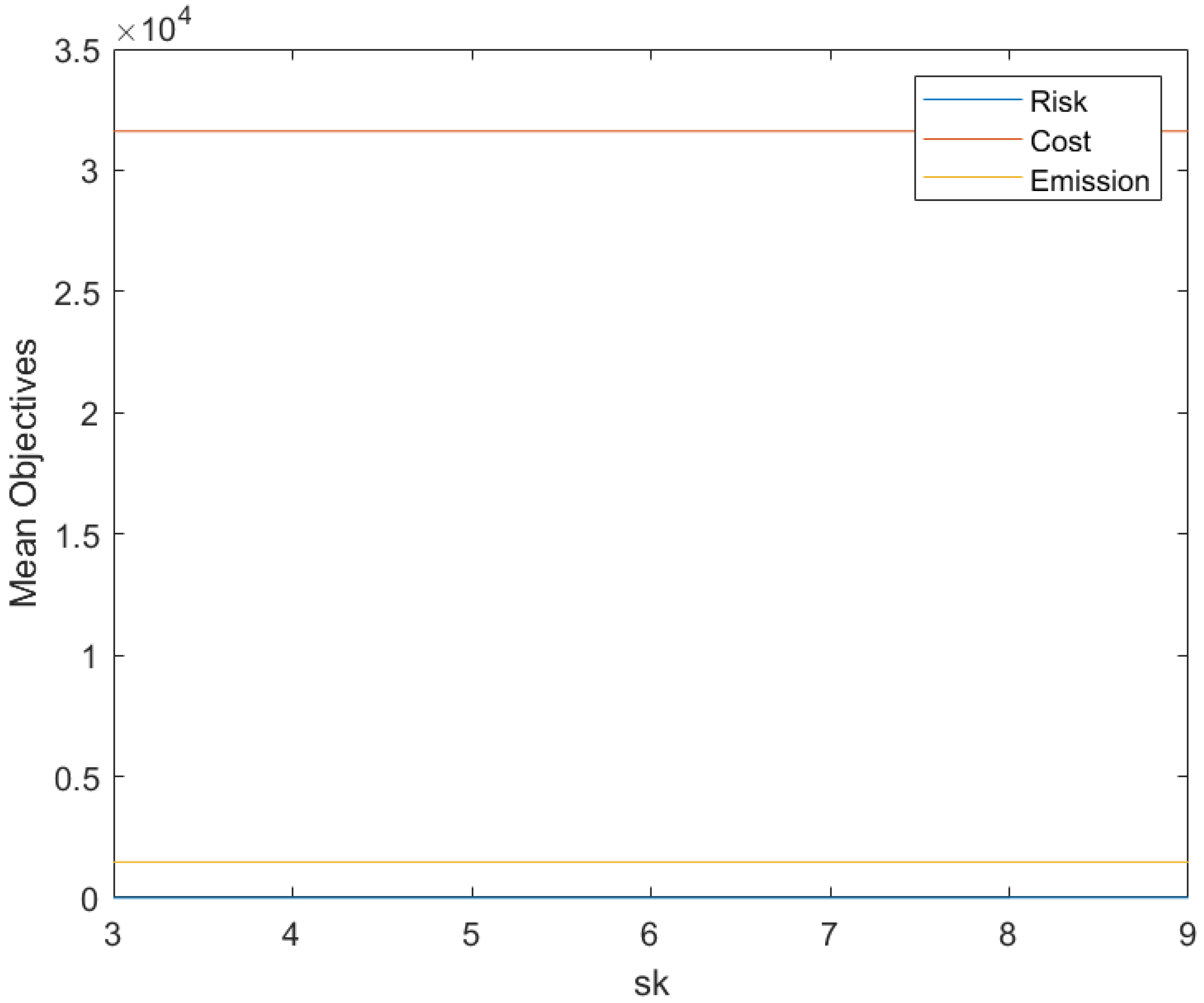
In the study of $s_k$ (tested with values of 3, 5, 7, 9),

Table 12. Sensitivity for $s_k$.

${\mathit{s}}_{\mathit{k}}$	Risk	Cost	Emission
3	1.6131	31,615.70	1474.86
5	2.6884	31,615.70	1474.86
7	3.7638	31,615.70	1474.86
9	4.8392	31,615.70	1474.86

and Figure 19 show that only the risk increases linearly, while the cost and emissions remain unchanged. This result is attributed to the independent role of $s_k$ in the risk objective function: increasing $s_k$ will amplify the perceived severity, but will not change economic or environmental factors. For example, raising $s_k$ from 5 to 9 will increase the risk value from 2.6884 to 4.8392, and the increase is close to the proportional relationship, which confirms the function of $s_k$ as a risk scaling coefficient. The stability of other objectives highlights the characteristics of the model, decoupling risks from costs and emission factors.

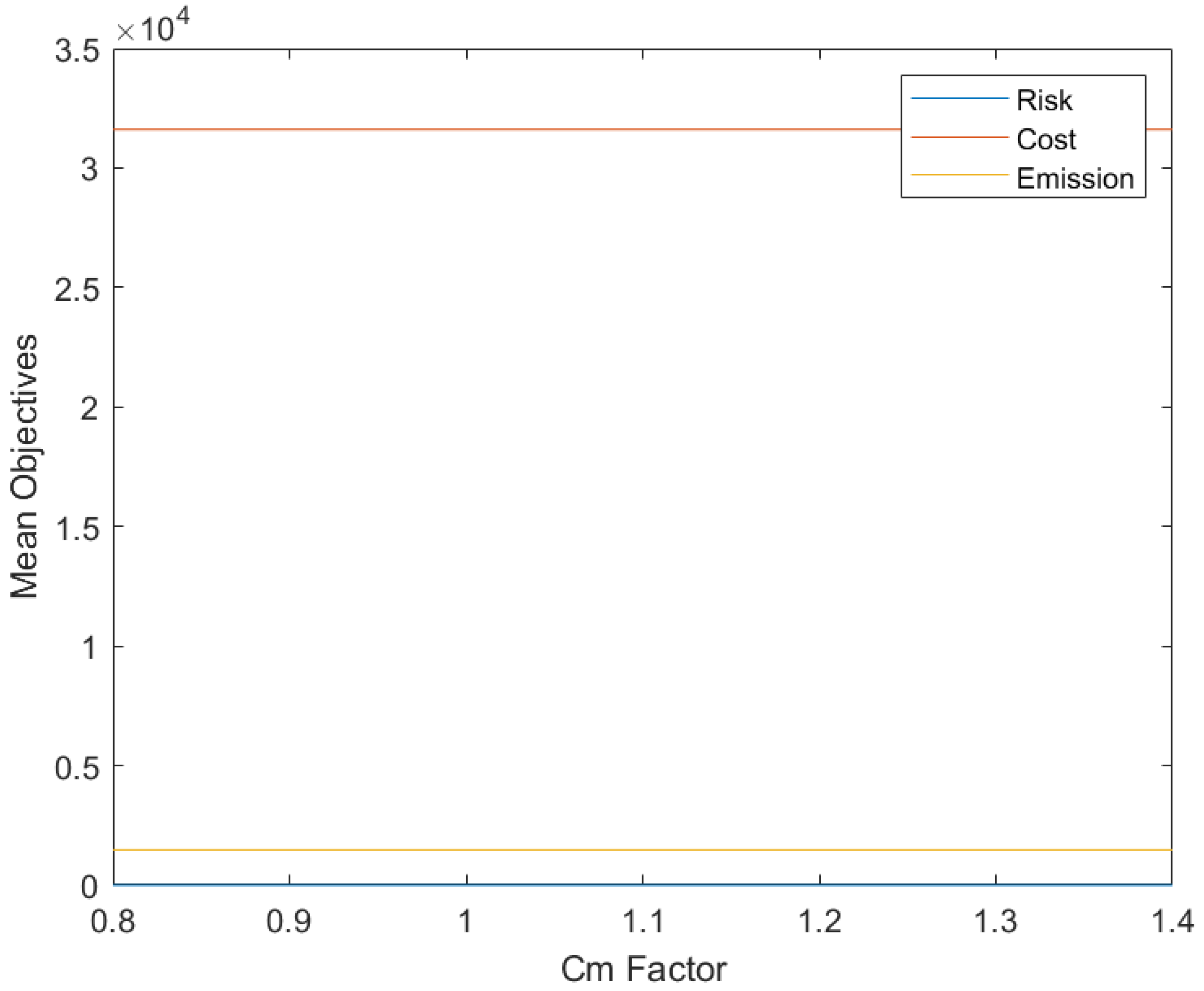
In the study of $C^m$ factors (test values are 0.8, 1.0, 1.2, 1.4),

Table 13. Sensitivity for Cm.

Cm Factor	Risk	Cost	Emission
0.8	2.6884	31,615.70	1474.86
1.0	2.6884	31,615.70	1474.86
1.2	2.6884	31,615.70	1474.86
1.4	2.6884	31,615.70	1474.86

and Figure 20 show that all objective values have no observable changes. This insensitivity comes from the fact that $C^m$ is mainly used as a capacity constraint in mode selection, rather than a direct influencing factor of the objective function, and its numerical fluctuations will not change the composition of the objective function. Therefore, the objective values are stable at risk 2.6884, cost 31,615.70, and emission 1474.86, which confirms the strong adaptability of the model to the fluctuation of transportation capacity.

The research results of the above section show that the model has good stability. Among them, the parameter Q has become the most influential variable because of its direct effect on cost and emissions and needs to be carefully calibrated in practical applications. The parameters $s_k$ and $C^m$ have limited influence, which further enhances the overall robustness of the model.

5. Conclusions

In response to the urgent challenges of hazardous materials transportation in the multimodal transportation network, this study puts forward a multi-objective optimization framework for coordinating safety risks, economic costs, and environmental emissions. This research builds a refined mathematical model based on realistic assumptions, such as deterministic parameters and flow conservation, which lays the foundation for evaluating the trade-off relationship in complex logistics scenarios. The improved I-NSGA-II algorithm efficiently generates diversified Pareto optimal solutions through customized exploration and development mechanisms, which is better than traditional methods in terms of convergence and solution quality. Sorting the deconsociation through the entropy power TOPSIS method, the framework achieves objective and data-driven optimal path selection. Through a case study from Berlin to Paris, it is shown that the method significantly reduces transportation risks and environmental emissions while maintaining cost-effectiveness.

From a practical perspective, the results provide actionable guidance for hazardous materials logistics enterprises and policymakers. Enterprises can directly implement the optimal route to reduce operating costs by 7.3% and emissions by 12.7% without compromising safety. Policymakers can utilize the model to evaluate and optimize regulatory bans, time-window policies, and mode capacity limits across European multimodal corridors, thereby enhancing supply chain resilience and public safety in real-world international hazardous materials transportation.

The main contributions of this study are as follows: (1) a three-objective optimization model incorporating real-world constraints, such as regulatory bans, time windows, and mode compatibility; (2) an improved NSGA-II with population invasion and homologous competition mechanisms that significantly enhances diversity and convergence; (3) integration of entropy-weighted TOPSIS for robust optimal route selection that aligns well with both objective data and subjective judgment; and (4) validation through a real Berlin–Paris case study, confirming superior performance over baseline NSGA-II and MOQPSO while offering practical insights for sustainable multimodal logistics.

Future research directions include extending the current model to simultaneously transport multiple types of hazardous goods and incorporating stochastic or fuzzy variables for accident probability and severity to better reflect real-world uncertainties such as weather variations and traffic disruptions. These extensions will further strengthen the framework’s applicability in complex and dynamic transportation environments.

References

1. Lecue, M.; Darbra, R.M. Accidents in European ports involving chemical substances: Characteristics and trends. Saf. Sci. 2019, 115, 278–284. [Google Scholar] [CrossRef]
2. Zou, Z.; Kang, S. Route Optimization for Hazardous Chemicals Transportation under Time-Varying Conditions. Sustainability 2024, 16, 779. [Google Scholar] [CrossRef]
3. Kengpol, A.; Tuammee, S.; Tuominen, M. The development of a framework for route selection in multimodal transportation. Int. J. Logist. Manag. 2014, 25, 581–610. [Google Scholar] [CrossRef]
4. Rondinelli, D.; Berry, M. Multimodal transportation, logistics, and the environment: Managing interactions in a global economy. Eur. Manag. J. 2000, 18, 398–410. [Google Scholar] [CrossRef]
5. Rajadurai, M.; Kaliyaperumal, P. Optimizing multimodal transportation: A novel decision-making approach with fuzzy risk assessment. IEEE Access 2025, 13, 14584–14610. [Google Scholar] [CrossRef]
6. Liu, J.; Xu, H.; Chen, J. The effects and conflicts of co-opetition in a rail-water multimodal transport system. Ann. Oper. Res. 2023, 1–46. [Google Scholar] [CrossRef]
7. Wang, Q.-Z.; Chen, J.-M.; Tseng, M.-L.; Luan, H.-M.; Ali, M.H. Modelling green multimodal transport route performance with witness simulation software. J. Clean. Prod. 2020, 248, 119245. [Google Scholar] [CrossRef]
8. Yin, C.; Zeng, L.; Fu, X.; Zhong, M. Transition of multimodal transport network under different carbon price scenarios. Transp. Policy 2025, 164, 1–26. [Google Scholar] [CrossRef]
9. Somsai, T.; Pongcharoen, P.; Hicks, C. Optimizing sustainable multimodal distribution networks in the context of carbon pricing, with a case study in the Thai sugar industry. Energy 2024, 298, 131273. [Google Scholar] [CrossRef]
10. Tsao, Y.-C.; Linh, V.T. Seaport-dry port network design considering multimodal transport and carbon emissions. J. Clean. Prod. 2018, 199, 481–492. [Google Scholar] [CrossRef]
11. Hu, X.; Cheng, R.; Zhao, J.; Zhou, X. Government subsidy-penalty strategy to promote low-carbon multimodal transportation using dynamic-static combination mechanism. Humanit. Soc. Sci. Commun. 2025, 12, 762. [Google Scholar] [CrossRef]
12. Mehrem, A.; Ding, S.L.; Noche, B. Optimization Analysis of Cold Chain Intermodal Transport Scheme for Agricultural Products Based on Carbon Emissions. In Proceedings of the 5th South American Conference on Industrial Engineering and Operations Management, Bogota, Colombia, 7–9 May 2024. [Google Scholar]
13. Binsfeld, T.; Hamdan, S.; Jouini, O.; Gast, J. On the optimization of green multimodal transportation: A case study of the West German canal system. Ann. Oper. Res. 2025, 351, 667–726. [Google Scholar] [CrossRef]
14. Lu, F.; Gao, Z.; Jiang, R.; Bi, H. Routing optimization of takeout delivery routes under joint delivery model of drones, occasional drivers, and riders. IEEE Trans. Intell. Transp. Syst. 2025, 26, 21784–21793. [Google Scholar] [CrossRef]
15. Huang, Y.; Li, T.; Ma, L. A multi-objective multimodal transportation route planning model considering fuzzy node loads. Int. J. Innov. Comput. Inf. Control 2024, 20, 1331–1350. [Google Scholar]
16. Huang, C.; Sun, H.; Liu, C.; Zhang, X.; Gao, T.; Tian, J. Research on container multimodal transportation multi-objective path optimization from hinterlands to shanghai port. IEEE Access 2025, 13, 32794–32807. [Google Scholar] [CrossRef]
17. Cheng, M.; Dong, L. An evolutionary multitasking ant colony optimization method based on population diversity control for multimodal transport problems. Int. J. Comput. Intell. Syst. 2024, 17, 159. [Google Scholar] [CrossRef]
18. Zhang, H.; Li, Y.; Zhang, Q.; Chen, D. Route selection of multimodal transport based on China railway transportation. J. Adv. Transp. 2021, 2021, 9984659. [Google Scholar] [CrossRef]
19. Cui, T.; Shi, Y.; Wang, J.; Ding, R.; Li, J.; Li, K. Practice of an improved many-objective route optimization algorithm in a multimodal transportation case under uncertain demand. Complex Intell. Syst. 2025, 11, 136. [Google Scholar] [CrossRef]
20. Zhang, T.; Cheng, J.; Zou, Y. Multimodal transportation routing optimization based on multi-objective Q-learning under time uncertainty. Complex Intell. Syst. 2024, 10, 3133–3152. [Google Scholar] [CrossRef]
21. Ru, S. Vehicle logistics intermodal route optimization based on Tabu search algorithm. Sci. Rep. 2024, 14, 11859. [Google Scholar] [CrossRef]
22. Faroqi, H. Multiobjective route finding in a multimode transportation network by NSGA-II. J. Eng. Appl. Sci. 2024, 71, 81. [Google Scholar] [CrossRef]
23. Qi, C. Multi-objective optimization-based algorithm for selecting the optimal path of rural multi-temperature zone cold chain dynamic logistics intermodal transportation. Int. J. Comput. Intell. Syst. 2024, 17, 224. [Google Scholar] [CrossRef]
24. Prakash, S.; Mehta, U.; Sharma, B. Artificial intelligence-driven multimodal route planning: Addressing dynamic unavailability and disruptions. IEEE Access 2024, 12, 172088–172100. [Google Scholar] [CrossRef]
25. Farahmand-Tabar, S.; Afrasyabi, P. Multi-modal routing in urban transportation network using multi-objective quantum particle swarm optimization. In Applied Multi-Objective Optimization; Springer: Singapore, 2024; pp. 133–154. [Google Scholar]
26. Feng, X.; Song, R.; Yin, W.; Yin, X.; Zhang, R. Multimodal transportation network with cargo containerization technology: Advantages and challenges. Transp. Policy 2023, 132, 128–143. [Google Scholar] [CrossRef]
27. Myronenko, V.; Yurchenko, O.; Vasilova, H. Multimodal logistics chains for international transportation of dangerous and perishable goods. MATEC Web Conf. 2024, 390, 03009. [Google Scholar] [CrossRef]
28. Liu, L.; Tian, T.; Wang, R.; Li, S. Time Varying Route Optimization of Hazardous Materials Transportation Considering Risk Equity. Preprint 2025. [Google Scholar] [CrossRef]
29. Chen, F.; Zhu, Q. Intelligent optimization method for hazardous materials transportation routing with multi-mode and multi-criterion collaborative constraints. Sci. Rep. 2025, 15, 7804. [Google Scholar] [CrossRef]
30. Yang, L.; Zhang, C.; Wu, X. Multi-objective path optimization of highway-railway multimodal transport considering carbon emissions. Appl. Sci. 2023, 13, 4731. [Google Scholar] [CrossRef]
31. Li, S.; Zu, Y.; Fang, H.; Liu, L.; Fan, T. Design optimization of a HAZMAT multimodal Hub-and-Spoke network with detour. Int. J. Environ. Res. Public Health 2021, 18, 12470. [Google Scholar] [CrossRef]
32. Keshavarzfard, R.; Naderi, A. A sustainable HazMat logistic network design considering scale of economy and route sensitivity and solving with Hybrid GA-SA. Int. J. Res. Ind. Eng. 2024, 13, 257–273. [Google Scholar]
33. Xie, L.; Cao, C. Multi-modal and multi-route transportation problem for hazardous materials under uncertainty. Eng. Optim. 2021, 53, 2180–2200. [Google Scholar] [CrossRef]
34. Galierikova, A.; Sosedova, J. Intermodal transportation of dangerous goods. Naše More 2018, 65, 8–11. [Google Scholar] [CrossRef]
35. Jia, H.; Li, J. Optimal Design of a Hazardous Materials Transportation Network considering Uncertainty in Accident Consequences. J. Adv. Transp. 2024, 2024, 1850690. [Google Scholar] [CrossRef]
36. Sun, M.; Zhou, R.; Jiao, C.; Sun, X. Severity analysis of hazardous material road transportation crashes with a Bayesian network using Highway Safety Information System data. Int. J. Environ. Res. Public Health 2022, 19, 4002. [Google Scholar] [CrossRef]
37. Mohammadfam, I.; Kalatpour, O.; Gholamizadeh, K. Quantitative assessment of safety and health risks in HAZMAT road transport using a hybrid approach: A case study in Tehran. ACS Chem. Health Saf. 2020, 27, 240–250. [Google Scholar] [CrossRef]
38. Liu, Q.; Zeng, Z.; Yang, D.; Liu, W.; Lu, X.; Zhou, L.; Jing, D. Multi-objective optimization and performance analysis of a CPV/T system based on NSGA-II and entropy weight TOPSIS method. Int. J. Heat Mass Transf. 2026, 255, 127810. [Google Scholar] [CrossRef]
39. Sadni, F.E.; Salhi, I.; Belhora, F.; Hajjaji, A. Multi-objective optimization of energy and exergy efficiencies in ORC configurations using NSGA-II and TOPSIS. Therm. Sci. Eng. Prog. 2025, 63, 103606. [Google Scholar] [CrossRef]
40. Asgari, M.; Ommi, F.; Saboohi, Z. Aeroelastic modeling and multi-objective optimization of a subsonic compressor rotor blade using a combination of modified NSGA-II, ANN, and TOPSIS. Results Eng. 2025, 26, 104615. [Google Scholar] [CrossRef]
41. Zhao, J.; Wei, W.; Zhao, L.; Xie, N.; Yang, T.; Jiang, K. Multi-objective optimization of PEMFC performance at different altitudes through integrated RSM, NSGA-II, EWM, and TOPSIS methodology. Int. J. Hydrogen Energy 2025, 177, 151615. [Google Scholar] [CrossRef]
42. Bergesen, H.O.; Parmann, G.; Thommessen, Ø.B. European agreement concerning the international carriage of dangerous goods by road (ADR). In Year Book of International Co-operation on Environment and Development; Routledge: London, UK, 2018; pp. 94–95. [Google Scholar]
43. European Environment Agency. Greenhouse Gas Emissions from Transport in Europe; European Environment Agency: Copenhagen, Denmark, 2019. [Google Scholar]
44. Serafimova, T. Decarbonizing freight transport in the European Union: Legal challenges and opportunities for shifting from road to rail. In Research Handbook on Climate Change and Infrastructure Law; Edward Elgar Publishing: Cheltenham, UK, 2025; pp. 335–369. [Google Scholar]
45. Deb, K.; Pratap, A.; Agarwal, S.; Meyarivan, T. A fast and elitist multiobjective genetic algorithm: NSGA-II. IEEE Trans. Evol. Comput. 2002, 6, 182–197. [Google Scholar] [CrossRef]
46. Deb, K.; Sundar, J. Reference point based multi-objective optimization using evolutionary algorithms. In 8th Annual Conference on Genetic and Evolutionary Computation; Association for Computing Machinery: New York, NY, USA, 2006; pp. 635–642. [Google Scholar]
47. Berens, P. CircStat: A MATLAB toolbox for circular statistics. J. Stat. Softw. 2009, 31, 1–21. [Google Scholar] [CrossRef]
Figure 1. Network diagram of random path layout for multimodal transportation.
Systems 14 00361 g001
Figure 2. Flowchart of the improved NSGA-II (I-NSGA-II) algorithm.
Systems 14 00361 g002
Figure 3. Example of encoding structure.
Systems 14 00361 g003
Figure 4. Example of PMX crossover.
Systems 14 00361 g004
Figure 5. Example of mutation.
Systems 14 00361 g005
Figure 6. Population invasion mechanism.
Systems 14 00361 g006
Figure 7. Homologous competition mechanism.
Systems 14 00361 g007
Figure 8. Hazardous materials transportation network topology in Europe.
Systems 14 00361 g008
Figure 10. Statistical power vs. sample size.
Systems 14 00361 g010
Figure 11. Improved NSGA-II metrics over generations.
Systems 14 00361 g011
Figure 12. NSGA-II metrics over generations.
Systems 14 00361 g012
Figure 13. MOQPSO metrics over generations.
Systems 14 00361 g013
Figure 14. Pareto frontier (risk vs. cost vs. emission).
Systems 14 00361 g014
Figure 15. Real–world validation: model vs. real distances.
Systems 14 00361 g015
Figure 16. Entropy weights.
Systems 14 00361 g016
Figure 17. Normalized scores.
Systems 14 00361 g017
Figure 18. Sensitivity for Q.
Systems 14 00361 g018
Figure 19. Sensitivity for s k .
Systems 14 00361 g019
Figure 20. Sensitivity for Cm.
Systems 14 00361 g020