AI-Based Demand Forecasting and Load Balancing for Optimising Energy Use in Healthcare Systems: A Real Case Study

Abstract

This paper addresses the critical need for efficient energy management in healthcare facilities, where fluctuating energy demands pose challenges to both operational reliability and sustainability objectives. Traditional energy management approaches often fall short in healthcare settings, resulting in inefficiencies and increased operational costs. To address this gap, the paper explores AI-driven methods for demand forecasting and load balancing and proposes an integrated framework combining Long Short-Term Memory (LSTM) networks, a genetic algorithm (GA), and SHAP (Shapley Additive Explanations), specifically tailored for healthcare energy management. While LSTM has been widely applied in time-series forecasting, its use for healthcare energy demand prediction remains relatively underexplored. In this study, LSTM is shown to significantly outperform conventional forecasting models, including ARIMA and Prophet, in capturing complex and non-linear demand patterns. Experimental results demonstrate that the LSTM model achieved a Mean Absolute Error (MAE) of 21.69, a Root Mean Square Error (RMSE) of 29.96, and an R² of approximately 0.98, compared to Prophet (MAE: 59.78, RMSE: 81.22, R² ≈ 0.86) and ARIMA (MAE: 87.73, RMSE: 125.22, R² ≈ 0.66), confirming its superior predictive performance. The genetic algorithm is employed both to support forecasting optimisation and to enhance load balancing strategies, enabling adaptive energy allocation under dynamic operating conditions. Furthermore, SHAP analysis is used to provide interpretable, within-model insights into feature contributions, improving transparency and trust in AI-driven energy decision-making. Overall, the proposed LSTM–GA–SHAP framework improves forecasting accuracy, supports efficient energy utilisation, and contributes to sustainability in healthcare environments. Future work will explore real-time deployment and further integration with reinforcement learning to enable continuous optimisation.

1. Introduction

Australia has a big capacity of using renewable energy in different regions [1,2]. Australian healthcare system plays a major role in using renewable energies. Optimising energy use in healthcare systems is essential due to the high and often unpredictable energy demands needed to run medical equipment, keep environmental conditions stable, and support constant patient care. Traditional energy management methods often don’t meet the complex needs of healthcare environments, where energy usage patterns can vary based on patient intake, equipment use, and seasonal factors [3].

AI-based demand forecasting offers a valuable solution by using past data, operational activities, and environmental conditions to accurately predict future energy needs [4]. This study contributes to the literature by developing an integrated AI-driven framework that merges demand forecasting techniques, including ARIMA, Prophet, and LSTM models, with Genetic Algorithm-based load balancing, aiming to optimize energy usage within healthcare facilities. Furthermore, the research utilizes SHAP analysis to enhance model interpretability, thereby offering valuable insights into the influence of key variables on energy demand predictions. It evaluates the performance of different forecasting models in conjunction with GA for load balancing, providing a comprehensive comparative analysis to identify the most efficient strategy. Additionally, the study introduces a hierarchical load balancing approach designed to enhance energy distribution efficiency and resilience across various levels of healthcare networks. In addressing existing research gaps, this work uniquely integrates AI-based forecasting with adaptive load balancing in a cohesive framework specifically tailored for healthcare energy management.

This research aims to explore how different demand forecasting models—ARIMA, Prophet, and LSTM—combined with a GA, can help manage energy use in healthcare facilities. The study’s goal is to identify the most effective model combination for predicting energy demand and balancing energy load efficiently, supporting cost savings and operational stability in healthcare settings. At the end, the following research questions are answered:

• How well do ARIMA, Prophet, and LSTM models perform in predicting energy demand for healthcare facilities?
• How does integrating GA with each forecasting model affect energy load balancing within healthcare settings?
• Which forecasting model combined with GA offers the most practical balance of prediction accuracy, load balancing efficiency, and cost savings?
• How can AI-driven energy management systems be effectively implemented in healthcare facilities for better resource use and sustainability?

In healthcare environments, energy usage does not follow stable or predictable patterns, because heating loads, lighting schedules, and equipment operation are driven by dynamic clinical activities, occupancy fluctuations, and climate variability. The proposed AI-based forecasting and optimisation framework is therefore used to quantify when, where, and how much reduction can be achieved under realistic operating conditions, rather than to identify the direction of the relationship. By integrating LSTM forecasting with a genetic algorithm for load balancing, the framework supports data-driven operational decisions, such as optimal load shifting, predictive heating schedules, and automatic adjustment of lighting intensity, which can be implemented without affecting clinical service quality. In this context, AI provides actionable and measurable recommendations for existing facilities, enabling targeted interventions and estimated savings, rather than only confirming an obvious causal relationship.

The rest of the paper is organised as follows. Section 2 presents the literature review, which highlights previous studies on demand forecasting and load balancing in energy management, showing where current research could improve. The methodology section explains the machine learning models, and optimisation techniques used to forecast energy demand and balance loads effectively. The results analysis section evaluates the performance of ARIMA, Prophet, and LSTM models, demonstrating LSTM’s superior predictive accuracy and the role of GA in optimising load balancing. The discussion interprets these findings in relation to the study’s aims, emphasising the impact of AI-driven forecasting on energy efficiency and cost reduction in healthcare settings. Finally, the conclusion and future work sections summarise the study’s contributions, highlighting the effectiveness of the proposed LSTM-GA framework and suggesting areas for further research, including real-time implementation and hybrid modelling approaches.

2. Literature Review

Healthcare facilities have high energy demands due to continuous patient care, medical equipment operation, and strict environmental controls. As energy costs rise and sustainability becomes more critical, healthcare facilities need smarter ways to manage energy [5].

Demand forecasting involves predicting future energy needs in healthcare facilities by analyzing historical data patterns [6]. Common forecasting methods include statistical models such as Autoregressive Integrated Moving Average (ARIMA), machine learning approaches like Long Short-Term Memory (LSTM) neural networks, and specialized time series tools like Prophet. Load balancing, on the other hand, refers to the distribution of energy usage across different departments or time periods to prevent overloads and maximize efficiency. GA are frequently employed for this purpose, as they iteratively search for optimal resource allocation by simulating natural selection processes [7]. Additionally, AI-driven optimization leverages machine learning and GA to allocate energy resources effectively based on real-time forecasts, enabling facilities to adjust to demand fluctuations, enhance energy utilization, and reduce costs [8].

Energy management in healthcare is complex because it must support lifesaving equipment and constant patient care without interruption. Initially, hospitals managed energy through manual adjustments and traditional statistical models, but these approaches couldn’t handle the complexity of demand patterns in healthcare [9]. With advancements in AI, researchers started using machine learning models for demand forecasting and optimisation algorithms for load balancing, offering a more efficient solution. Historically, ARIMA and other traditional time series models were the go-to for demand forecasting, as they’re straightforward and perform well with linear data [10]. However, neural networks like LSTM have gained attention for their ability to capture long term patterns and dependencies, making them suitable for more complex, non-linear demand trends in healthcare. Similarly, GA were initially used in manufacturing and logistics for resource allocation, but their flexibility and adaptability make them well suited to managing energy needs in dynamic environments like healthcare [11].

Load balancing is another essential part of energy management in healthcare. It distributes energy loads across departments and different time frames, preventing overloads and making resource use more efficient [12]. Dynamic load balancing algorithms, inspired by grid computing, reallocate energy based on real time usage, forecasted needs, and renewable energy availability. Adaptive load balancing techniques, such as those used in Software Defined Networking (SDN), could inform healthcare load balancing by automatically redistributing energy to prevent any single department from being matched to current demand, avoiding power disruptions and ensuring the system runs smoothly [13].

By using AI-powered demand forecasting, healthcare facilities can better prepare for high demand periods, allocate resources more efficiently and keep energy costs down [14]. Hybrid forecasting approaches that combine machine learning models like LSTM with traditional methods offer even more accuracy. These are especially helpful in healthcare settings with intermittent or unpredictable energy needs, as hybrid models allow systems to handle complex demand patterns more flexible and avoid both under and overuse of resources [15].

For resilient and flexible energy management, AI driven hierarchical load balancing models help optimise distribution across local, group, and network levels. Adapted from distributed grid computing models, these systems allow healthcare facilities to scale energy allocation according to their size and needs, lowering communication costs and response times while maximising energy use. By organising load balancing hierarchically, healthcare systems meet energy demands at local (within a facility), group (across facilities), and network levels efficiently. This layered approach also decreases the likelihood of widespread disruptions, as energy loads are adjusted in real time across different levels [12].

By combining AI-based demand forecasting with adaptive load balancing, healthcare facilities gain a complete energy management system that improves both operational efficiency and sustainability. Genetic algorithm (GA) and Reinforcement Learning (RL) give the system adaptive abilities, enabling it to respond to fluctuations in demand in real time. These AI driven strategies enhance operational reliability while supporting environmental goals by making better use of renewable energy sources and reducing reliance on traditional energy supplies. Aligning AI driven forecasting with load balancing allows healthcare facilities to maintain energy stability, cut costs, and work toward sustainability. This approach highlights how AI advancements are providing healthcare with scalable, adaptable, and environmentally friendly energy solutions [16].

Machine learning models, particularly neural networks, have demonstrated superior performance in energy forecasting compared to traditional models, as highlighted by [4]. Their study underscores how advanced algorithms can effectively predict energy demand patterns in dynamic environments. Similarly, [17] emphasized that Long Short-Term Memory (LSTM) networks are particularly effective in capturing healthcare-specific demand fluctuations, achieving higher accuracy than simpler forecasting models by identifying complex temporal dependencies [17].

Load balancing models have also gained prominence in energy management contexts. Patni and Aswal [12] explored distributed load balancing in grid computing, which has since inspired adaptations for energy management in healthcare. Additionally, [13] examined the application of adaptive load balancing, as seen in Software Defined Networking (SDN), to real-time energy distributions. Their findings suggest that dynamically adjusting energy allocations based on current demand can significantly enhance system efficiency and resilience.

GA have proven particularly effective in optimizing energy resource management, given their capacity to handle complex and dynamic requirements. Hameed et al. [16] demonstrated that GA’s adaptability to real-time adjustments allows for effective load balancing, making them particularly suitable for unpredictable energy demands in healthcare settings. Their study confirms that GA can optimize energy distribution effectively, accounting for both demand fluctuations and operational constraints.

As summarised in

Table 1. Comparison of Previous Studies vs. This study.

Study	Model	Key Findings	Limitations	Improvements in This Study
[4]	Neural Networks	Machine Learning models outperform traditional forecasting models	Lacked optimisation for real time load balancing	Integrated GA for dynamic load balancing
[17]	LSTM	LSTM effectively captures healthcare energy demand fluctuations	Lacks explainability and real time adaptability	Used SHAP for interpretability and GA for optimisation
[12]	Grid-based load balancing	Load balancing models improve resource distribution	Did not incorporate forecasting for predictive energy allocation	Incorporated LSTM forecasting for proactive energy balancing
[13]	Adaptive load balancing	Real time load balancing enhances energy efficiency	Did not use demand forecasting to predict the optimise loads	Combined LSTM forecasting with GA for demand aware load balancing
[16]	GA based load balancing	GA effectively optimises energy distribution	Did not integrate forecasting for proactive energy allocation	Used LSTM-GA integration for predictive and adaptive energy management
This Study	LSTM, ARIMA, Prophet, and GA with SHAP interpretability	Combines forecasting, optimisation, and interpretability for a comprehensive AI driven energy management approach	Addresses previous gaps in real time adaptability, forecasting accuracy, and explainability	Provided an integrated, scalable, and interpretable solution tailored for healthcare energy management

, traditional models like ARIMA perform well for stationary and linear data but struggle with capturing complex, non-linear demand patterns commonly found in healthcare energy usage. Prophet improves upon ARIMA by handling missing data and seasonal variations more effectively but remains limited in highly irregular demand scenarios. LSTM, demonstrated superior accuracy in modelling long-term dependencies and non-linear trends; however, its higher computational costs and need for extensive parameter tuning highlight the importance of optimisation techniques like GA to enhance efficiency and ensure practical deployment in real world healthcare settings.

The current study combines ideas from time series forecasting and evolutionary algorithms for an integrated approach. Time Series Forecasting is essential in predicting future data points based on historical data.

Table 2. Forecasting Model Comparisons.

Model	Description	Strengths	Limitations
ARIMA	A statistical model used for analysing and forecasting time series data, effective for linear trends [10]	Works well with stationary and linear data. Easy to interpret and implement. Requires minimal computational power.	Struggles with non-linear and complex demand patterns. Requires data preprocessing (stationarity and differencing)
Prophet	A forecasting model developed by Facebook, designed to handle seasonality and missing data, suitable for demand patterns that vary seasonally.	Handles missing data well. Captures seasonality and trend changes automatically. Requires minimal parameter tuning.	May struggle with highly irregular and non-seasonal patterns. Less effective for very short-term forecasting
LSTM	A deep learning model designed to recognize patterns in sequential data, making it useful for complex time series forecasting [18]	Captures long term dependencies. Handles complex, non-linear relationships. Adaptable to large and irregular datasets.	High computational cost. Requires large datasets and tuning. Less interpretable than traditional models.

provides forecasting model comparison used in the current study: For example, Table 2:

For load balancing, GA provides a structure where various potential solutions (i.e., ways to allocate energy) evolved over iterations to find the most optimal distribution based on forecasted demands.

In recent years, there has been a shift toward combining multiple forecasting and optimisation techniques for a hybrid approach to energy management. Many studies pair traditional statistical models with machine learning to capture both linear and non-linear patterns in demand [19]. However, while much research has focused on improving forecasting accuracy, fewer studies have examined how well different forecasting models perform when paired with optimisation algorithms like GA in healthcare. This study will address these gaps by testing three forecasting models—ARIMA, Prophet, and LSTM—with GA to find the best-performing combination for balancing energy loads in healthcare settings.

Key debates include whether complex machine learning models are worth the extra computing resources compared to traditional methods. Some researchers argue that models like LSTM are highly accurate but can be overkill due to the computational demands and lack of interpretability [3]. Similarly, GA and other optimisation techniques can be complex to implement, leading some to advocate for simpler, rule-based approaches in healthcare.

The current study will examine how AI-based forecasting and load balancing methods can improve energy efficiency in healthcare. A literature review here helps establish the concepts, past research, and current developments in this area, providing a foundation for identifying research gaps and areas for improvement.

Building on this existing research, this study evaluated three demand forecasting models (ARIMA, Prophet, LSTM) paired with a GA to balance energy loads effectively in healthcare. By comparing the accuracy and efficiency of each combination, this research will help determine which forecasting model is most practical and effective when used alongside GA for energy management.

3. Research Methodology

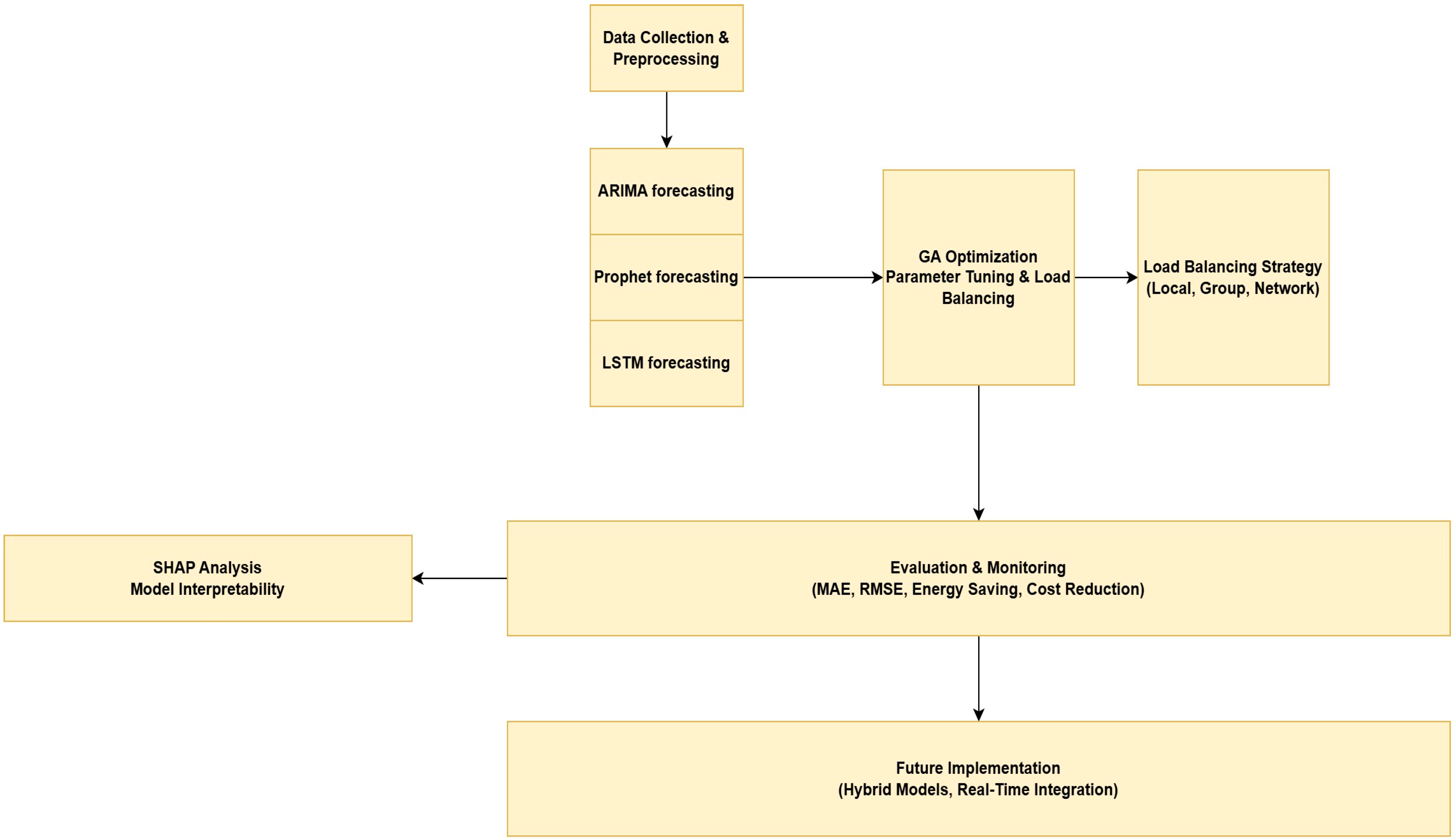
The flowchart, Figure 1, presents a structured framework for AI-driven energy management in healthcare facilities, comprising five key components. To further interpret the forecasting models and gain insights into their decision-making processes, SHAP (Shapley Additive Explanations) analysis is employed. SHAP values help explain the contribution of each feature in the prediction of energy demand by quantifying the impact of different inputs, such as historical energy usage, environmental conditions, and operational factors [20]. By applying SHAP analysis to the ARIMA, Prophet, and LSTM models, this study offers a clearer understanding of how each model interprets the data, allowing for more transparent and interpretable forecasting. This method not only highlights the importance of specific features but also reveals potential biases in the models, making it a valuable tool for enhancing the accuracy and reliability of energy demand predictions in healthcare environments.

The process begins with Data Collection & Preprocessing, which serves as the input for three forecasting models: ARIMA, Prophet, and LSTM, each designed to predict energy demand based on historical data. The forecasting outputs are then fed into the GA Optimization Parameter Tuning & Load Balancing module, which optimizes load allocation across multiple levels (Local, Group, Network) using GAs. The SHAP Analysis module interprets the forecasting model outputs, providing insights into feature importance and model behavior. The framework proceeds to the Evaluation & Monitoring phase, where key metrics such as MAE, RMSE, R², energy savings, and cost reduction are assessed to validate model performance. Finally, the Future Implementation stage outlines potential enhancements, including hybrid model integration and real-time deployment, ensuring scalability and adaptability in dynamic healthcare settings.

The hyperparameters of the GA were selected based on the role of GA within the proposed framework and the size of the corresponding search space. When GA was employed for load balancing and forecast-driven optimisation (e.g., ARIMA- and Prophet-based scheduling), a relatively larger population size and number of generations (population size = 20, generations = 100) were used to adequately explore the continuous solution space and ensure convergence toward stable allocation schedules.

In contrast, when GA was applied for hyperparameter tuning of learning models, the search space consisted of a small number of discrete candidate values (e.g., number of layers, neurons, or seasonal parameters). In these cases, a lightweight GA configuration (population size = 5, number of parents = 3, generations = 5, number of genes = 4) was sufficient to efficiently identify near-optimal configurations without excessive computational cost. This adaptive selection of GA hyperparameters balances optimisation accuracy and computational efficiency and is consistent with common practices in evolutionary optimisation.

3.1. Data Exploration

This study analyses energy consumption data from a hospital in Perth to understand usage patterns and identify potential efficiency improvements. Perth, shown in Figure 2, was selected as the focus of this study due to its unique climate, energy pricing structure, and healthcare infrastructure challenges. Unlike cities on the east coast, Perth experiences hot, dry summers and mild winters, creating distinct heating and cooling demands in healthcare facilities [21]. Additionally, Western Australia operates on a separate energy grid (the SWIS), which makes energy optimisation particularly important to ensure resilience and cost efficiency [22]. Hospitals are among the highest energy-consuming public facilities, and studying one in Perth offers insights into how building operations can be improved in similarly isolated or resource sensitive environments.

The dataset used was sourced from the NSW Government Open Data portal [24]. While the platform is an official and trustworthy government source, the dataset itself id not openly downloadable and requires a formal data request. This controlled access supports data integrity and privacy, adding to its reliability. This dataset includes hourly measurements of electricity and gas usage across various facility components. To support visualisation and pattern recognition, SAS Visual Analytics (trial version) was employed to generate bar charts, parallel coordinate plots, and correlation matrices that highlight significant relationships among variables.

The energy dataset used in this study was obtained from the hospital’s building energy management system (BEMS), which provides disaggregated energy consumption data for major end-use categories, including facility-level electricity and gas usage, interior equipment, lighting, water heating, and heating-related gas consumption. While not all subsystems are equipped with fully independent physical meters, the reported end-use values are derived from a combination of sub-metered measurements and system-level allocation methods commonly employed in hospital energy monitoring systems. As a result, the disaggregated profiles reflect operationally meaningful energy-use patterns suitable for demand forecasting and optimisation, rather than raw measurements from standalone meters for every sector.

The dataset consists of hourly operational energy records collected from a large hospital facility. The dataset includes electricity-related variables such as facility load, cooling electricity, fan electricity, interior equipment load, and interior lighting, as well as gas-related variables including facility gas consumption, heating gas, interior gas equipment usage, and water heater gas demand.

A preliminary analysis of the dataset reveals clear daily and weekly seasonal patterns, particularly in the electricity facility load, which tends to peak during daytime operational hours. Cooling loads show strong seasonal variability corresponding to warmer months, while heating-related gas usage increases in colder periods. To enhance interpretability, we provide summary distributions for each energy variable, showing their range, central tendency, and variability. These visualizations help illustrate the skewness, peak usage conditions, and differences in usage behavior between electricity and gas components.

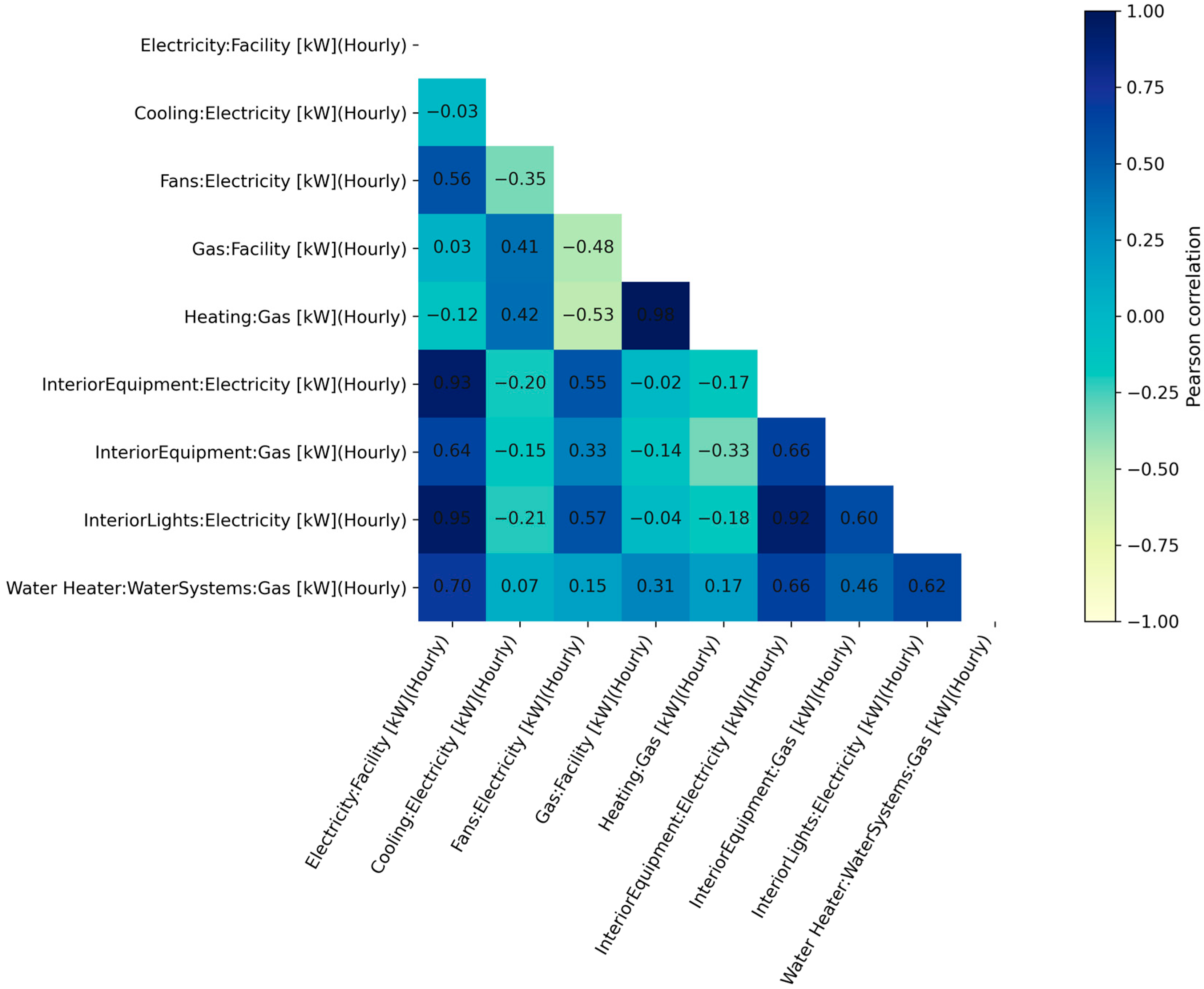
Figure 3 presents the Pearson correlation matrix computed from the hourly energy consumption data of the facility. Prior to analysis, all energy streams (electricity and gas) were aggregated at an hourly resolution and aligned in time to ensure consistency across end-use categories. Pearson’s correlation coefficient was then calculated for each pair of variables to quantify the strength and direction of their linear relationships. The results reveal a near-perfect correlation between gas consumption and heating demand (r = 0.98), indicating that gas usage in the facility is predominantly driven by space-heating requirements. In contrast, electricity consumption exhibits strong correlations with interior lighting (r = 0.95) and interior equipment loads (r = 0.93), suggesting that these end-uses are the primary contributors to overall electrical demand. A strong interrelationship is also observed between interior lighting and interior equipment (r = 0.92), implying concurrent operation patterns during occupied periods.

Moderate correlations are observed between water heating gas consumption and electrical end-uses, reflecting indirect operational coupling rather than direct dependency. Cooling electricity demand shows relatively weak correlations with other variables, indicating that cooling loads are governed by different drivers, such as ambient temperature and occupancy dynamics. Overall, Figure 4 highlights the dominant role of heating in gas consumption and the central contribution of lighting and equipment to electricity demand. These findings support targeted energy-management strategies focusing on heating optimisation, as well as energy-efficient lighting and equipment scheduling, to achieve effective reductions in both gas and electricity usage.

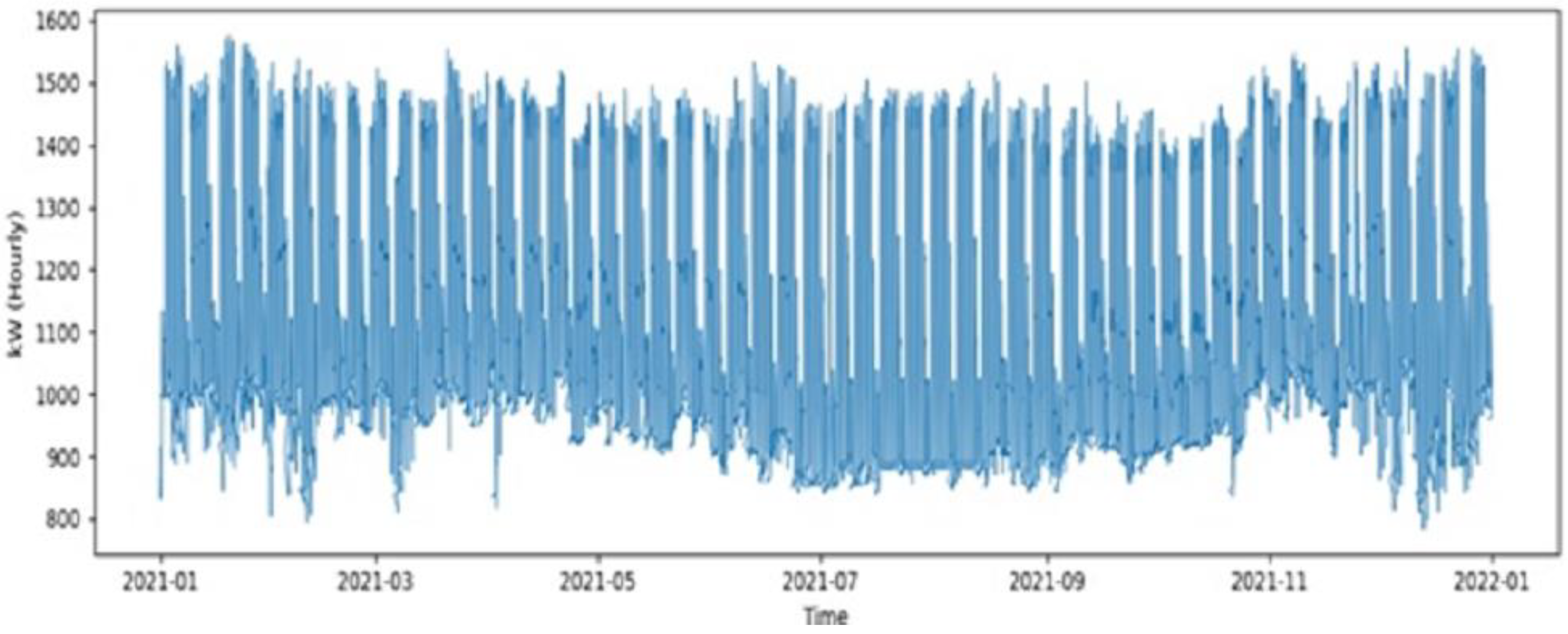
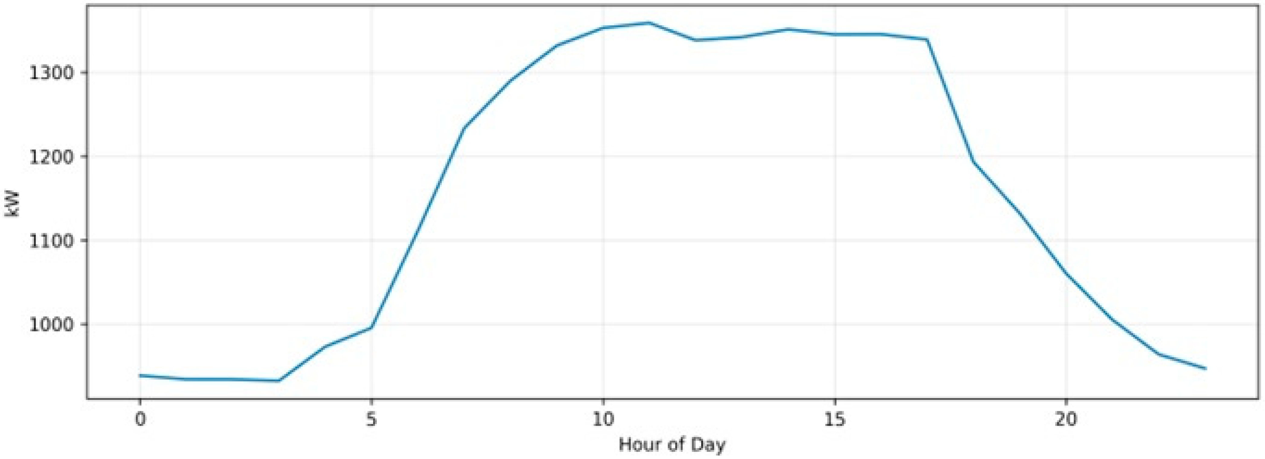
Figure 4 shows the full-year hourly electricity facility load, revealing strong daily oscillations and longer-term seasonal variations, with higher overall demand during warmer months. Figure 5 illustrates the average daily load profile, where consumption increases sharply during early working hours, peaks between mid-morning and late afternoon, and gradually declines overnight, reflecting typical hospital operational cycles. 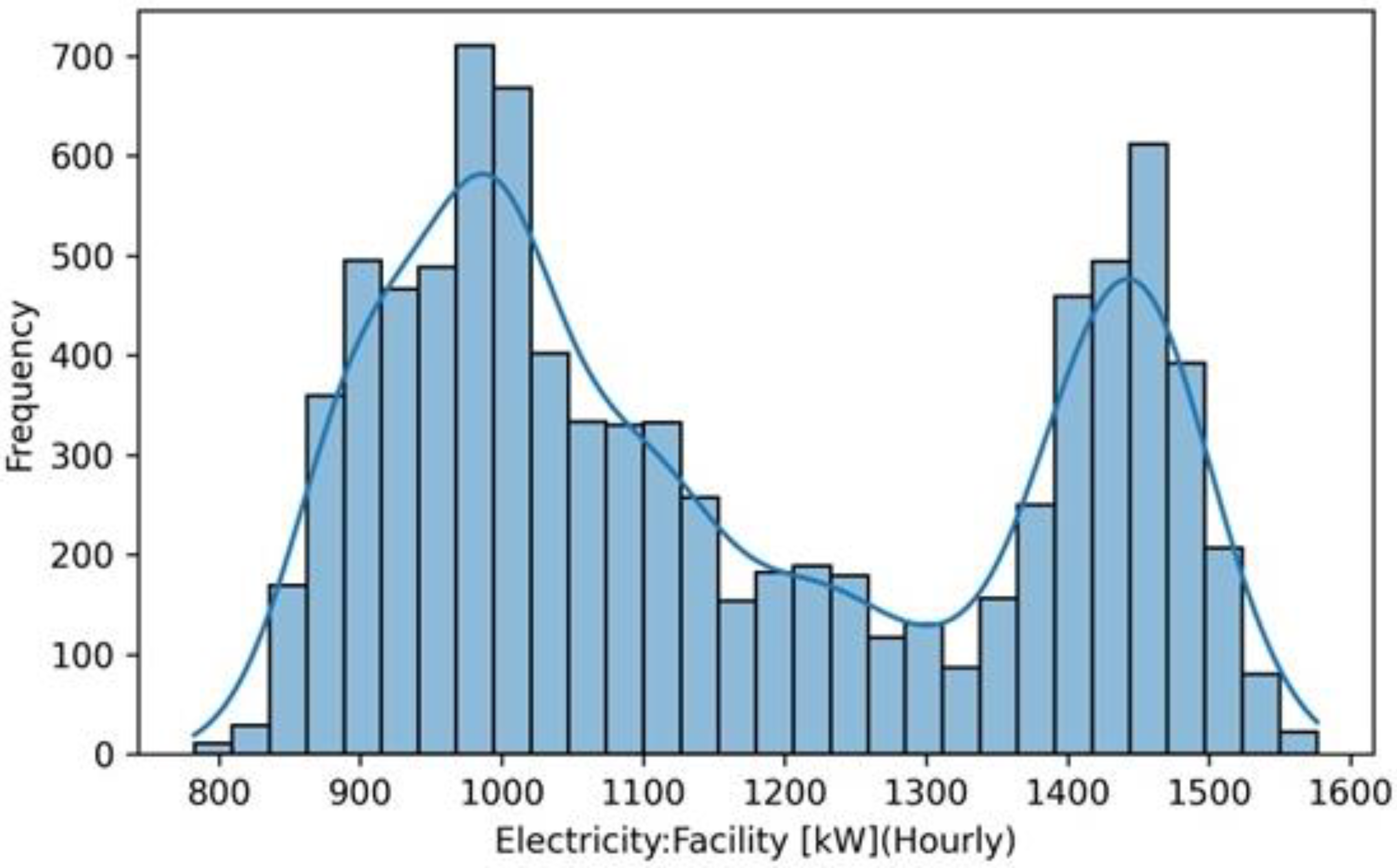Figure 6 presents the distribution of hourly electricity loads, showing a multimodal pattern driven by differing daytime, nighttime, and seasonal operating conditions. Together, these visualizations provide a comprehensive understanding of the temporal span, seasonal behavior, and statistical distribution of the dataset, addressing the reviewer’s request for richer dataset characterization.

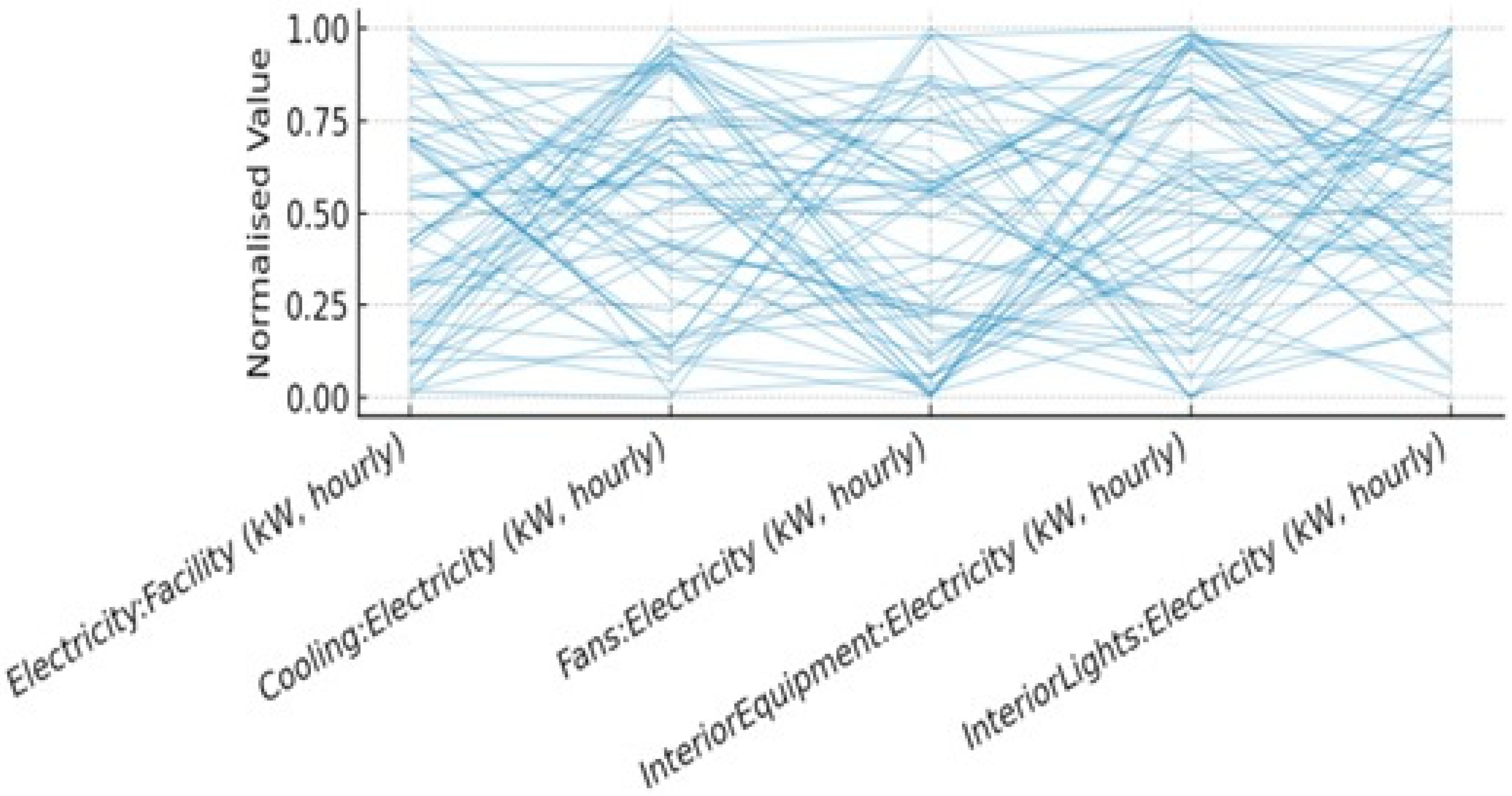
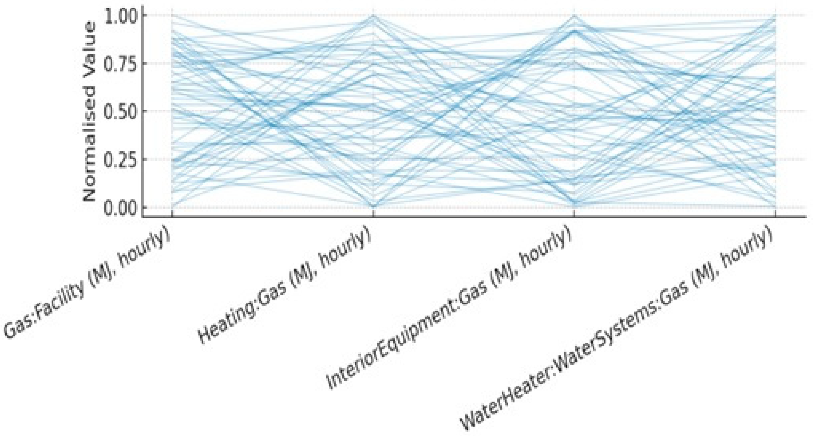
Through the bar chart in Figure 7, and the parallel coordinate graphs in Figure 8 and Figure 9, we can see that Electricity is strongly influences by Interior Lights (Importance of 1.000) and Interior Equipment (Importance of 0.946), with these two variables showing the highest correlations. This indicates that changes in lighting and equipment usage significantly drive the total electricity demand within the facility. The data shows that higher levels of interior lighting usage, particularly around the commonly observed values of 243.26 kW, are associated with higher overall electricity consumption. Meanwhile, interior equipment usage also consistently contributes to the facility’s power demands, suggesting it represents a steady operational load. Fans and cooling also correlate with facility electricity usage, though to a lesser extent, highlighting their role in ventilation and environmental control. While cooling demand may vary seasonally, fan usage appears to be more consistent, likely driven by HVAC system requirements. This analysis suggests that focusing on lighting and equipment optimisation, possibly through automated control systems or operational scheduling, could be effective strategies to reduce total electricity demand without compromising functionality.

This parallel coordinate plot in Figure 9, shows the gas consumption patterns for the facility across three primary sources: Heating, Interior Equipment, and Water Heater. Heating dominates gas consumption, indicating that space heating likely represents the bulk gas usage. Interior Equipment and Water Heater have much lower and more consistent usage levels, suggesting they contribute minimally to overall gas demand. The similarity between Gas Facility and the Heating, also supports the fact that majority of the gas is used by Heating. Efficiency improvements targeting Heating could have a significant impact on reducing overall gas demand, while adjustments in Interior Equipment and Water Heater would likely yield smaller savings.

This analysis, based on data visualised with SAS Visual Analytics, reveals distinct patterns in energy usage within the hospital. The high correlation between gas and heating, and between electricity, lighting, and equipment, suggests targeted areas for energy optimisation. This methodology provides a foundation for developing strategies to manage electricity and gas usage more efficiently, which could lead to cost savings and reduced environmental impact for healthcare facilities.

3.2. Implementation

In this research study, a framework for energy demand forecasting and load balancing in healthcare facilities is developed by integrating three advanced forecasting models—ARIMA, Prophet, and LSTM—along with GA for load balancing. The methodology followed throughout the study is structured into distinct phases: model development, integration, and evaluation.

3.3. Model Development and Integration

Three different forecasting models were used in this study: ARIMA, Prophet, and LSTM, each chosen for their unique strengths in time series analysis.

3.3.1. ARIMA Model (Autoregressive Integrated Moving Average)

The ARIMA model was implemented using Python’s (version 3.10) statsmodels library to capture linear trends in historical energy consumption data. The dataset, which contained electricity usage at hourly intervals, was pre-processed by converting timestamps into a datetime format, forward-filling missing values to maintain data continuity, and setting the ‘Date/Time’ column as the index for time series analysis.

The model was configured with the following hyperparameters:

-

p (autoregressive order): 2

-

d (differencing order): 1

-

q (moving average order): 2

The ARIMA model was trained on the pre-processed time series data to predict future electricity demand over a 48 h forecast horizon. The model’s performance was evaluated using Mean Absolute Error (MAE) to measure the average magnitude of errors in predictions and Root Mean Squared Error (RMSE) to emphasise larger errors, highlighting extreme mismatches between actual and predicted values. Algorithm 1 presents the ARIMA forecasting with GA-based load optimization. The hyperparameters of all forecasting models were tuned using a separate validation subset of the data. For each model, we defined a discrete search space of candidate values and selected the configuration that minimised the validation RMSE.

Table 3. Hyperparameters and tuning strategy for the forecasting models.

Model	Hyperparameter	Description	Search Range/Candidates	Tuning Strategy
ARIMA	p	Autoregressive order	{1, 2, 3, 4, 5}	Grid search on validation set (min RMSE)
	d	Differencing order	{0, 1}
	q	Moving-average order	{1, 2, 3, 4}
Prophet	changepoint_prior_scale	Flexibility of trend changes	{0.01, 0.05, 0.1, 0.5}	Grid search on validation set (min RMSE)
	seasonality_prior_scale	Strength of seasonal components	{1, 5, 10}
	Seasonality	Included seasonal terms	{daily, weekly, yearly, weekly + yearly}
LSTM	Number of layers	Depth of LSTM network	{1, 2}	Random/grid search on validation set
	Hidden units per layer	Width of LSTM layer	{32, 64, 128}
	Look-back window	Number of past hours as input	{24, 48, 72}
	Batch size	Training mini-batch size	{32, 64, 128}
	Learning rate	Step size for optimiser	{0.001, 0.0005}
	Epochs	Max training iterations	{50, 100}	Early stopping on validation loss

summarizes the tuned hyperparameters for ARIMA, Prophet, and LSTM, including their search ranges, selected values, and the adopted tuning strategy. This separation of algorithmic steps from hyperparameter configuration improves the transparency and reproducibility of the proposed framework.

Algorithm 1. Pseudocode: ARIMA Forecasting with GA-based Load Optimization (48 h horizon)

Input: time series $y_t$, forecast horizon $H=48$, GA settings, ARIMA hyperparameters from Table 1 Output: forecast ${\widehat{y}}_{t+1:t+H}$, optimized load allocation $x_{1:H}^{\ast }$ Pseudocode:         1. Preprocess data ○ Parse timestamps, set Date/Time as index, forward-fill missing values (if any).         2. Select ARIMA hyperparameters ○ Choose $\left(p,d,q\right)$ using validation search space in Table 1 (final selected values reported in the text: $p=2, d=1,q=2)$         3. Fit ARIMA and forecast ○ Fit ARIMA $\left(p,d,q\right)$ on training series $y_t$ ○ Generate forecast ${\widehat{y}}_{1:H}$ for the next 48 h.         4. GA-based load balancing (optimize allocation around forecast) ○ Initialize population: generate candidate allocations $x_{1:H}^{\left(i\right)}$ within $\left[0.8\widehat{y},1.2\widehat{y}\right]$ ○ Fitness: $F(x)=-{\sum }_{h=1}^H\mid x_h-{\widehat{y}}_h\mid$ (maximize fitness = minimize deviation). ○ For generation $g=1$ to $G$ (e.g., 100): ▪ Compute fitness for all individuals. ▪ Select parents (tournament selection). ▪ Crossover (SBX) → offspring. ▪ Mutation (Gaussian noise with adaptive probability). ▪ Replace worst individuals with offspring. ○ Return best allocation $x_{1:H}^{\ast }.$

3.3.2. Prophet Model

The Prophet model, developed by Facebook, was utilised for its ability to handle seasonal patterns, holiday effects, and trend changes, making it particularly suitable for healthcare energy forecasting. The dataset was reformatted to match Prophet’s expected structure by renaming columns to ‘ds’ (date) and ‘y’ (energy consumption). Outliers (values beyond three standard deviations from the mean) were removed to prevent extreme data points from skewing the forecast.

The Prophet model’s changepoint prior scale (which adjusts the flexibility of trend changes) and seasonality prior scale (which controls the strength of seasonal patterns) were optimised using GA. The GA iteratively refined parameter sets over 50 generations to minimise the RMSE of Prophet’s predictions. Algorithm 2 presents the Prophet forecasting with GA-based load optimization.

Algorithm 2. Pseudocode: Prophet Forecasting with GA-based Load Optimization

Input: timestamped data $\left(ds,y\right)$, Prophet hyperparameter search space, tuning generations $G_p=50$, load-balancing horizon $H$ (plots use ~50 h), GA load-balancing generations $G$ Output: tuned Prophet model, forecast $\widehat{y}$, optimized allocation $x^{\ast }$ Pseudocode:         1. Preprocess data for Prophet ○ Create dataframe with columns ds (datetime) and y (energy demand) ○ Remove outliers beyond 3 standard deviations (as stated).         2. GA hyperparameter tuning for Prophet (50 generations) ○ Decision variables: ▪ changepoint_prior_scale, seasonality_prior_scale, and seasonality set. ○ Objective: minimize validation RMSE. ○ Initialize population of candidate Prophet configurations. ○ For generation $g=1$ to 50: ▪ For each candidate configuration: fit Prophet on training split, forecast on validation split, compute RMSE. ▪ Apply selection + crossover + mutation to create new candidates. ○ Select best Prophet configuration ${\theta }^{\ast }$         3. Fit final Prophet and forecast ○ Fit Prophet $\left({\theta }^{\ast }\right)$ on full training data. ○ Forecast future demand for horizon $H$ (e.g., first 50 h used for downstream optimization in the workflow).         4. GA-based load balancing ○ Initialize allocations within $\left[0.8\widehat{y},1.2\widehat{y}\right]$ ○ Fitness: minimize deviation from forecast. ○ Run GA for $G$ generations (e.g., 100) and output $x^{\ast }$.

3.3.3. LSTM Model (Long Short-Term Memory)

The LSTM model was selected for its ability to capture non-linear relationships and long-term dependencies in time series data. The implementation was conducted using TensorFlow and Keras. The dataset was scaled using MinMaxScaler to normalise energy consumption values between 0 and 1, facilitating faster convergence during training. Time series sequences were generated using a sliding window approach, where the past 24 h of energy usage were used to predict the next hour. The choice of a 24 h lag was based on domain knowledge and an autocorrelation plot, which showed strong correlations between current energy consumption and the previous 24 h. This aligns with daily operational cycles in healthcare facilities, where energy usage patterns typically repeat every 24 h due to staff shifts, equipment usage, and patient intake cycles.

The LSTM model was structured with:

-

Two LSTM layers: The first layer returned sequences for stacking, while the second produced the final output.

-

Dropout layers: Inserted after each LSTM layer to prevent overfitting.

-

Dense layers: Applied to produce the final prediction.

After training for 50 epochs, the model’s performance was assessed using MAE, R², and RMSE. Algorithm 3 presents the LSTM forecasting with GA-based load optimization.

Algorithm 3. Pseudocode: Hyperparameter Tuning of LSTM using Genetic Algorithm

Input: time series $y_t$, look-back $L=24$, LSTM search space (Table 1), GA tuning iterations, GA load balancing Output: tuned LSTM model, forecasts, optimized allocation Pseudocode:         1. Preprocess & sequence construction ○ Scale $y_t$ using MinMaxScaler. ○ Create supervised sequences using look-back $\mathbf{L} \mathbf{=} \mathbf{24}: \mathrm{input} X_t=[y_{t-L},\dots ,y_{t-1}]$, target $y_t$. ○ Split into train/validation/test sets.         2. GA hyperparameter tuning for LSTM (search space from Table 1) ○ Decision variables (Table 1): #layers, hidden units, look-back (if tuned), batch size, learning rate, epochs, etc. ○ Fitness: negative validation RMSE (or MAE), computed after a short training budget per candidate (to keep tuning efficient). ○ Initialize population of candidate LSTM configurations. ○ For each generation: ▪ For each candidate: build LSTM, train on training data, evaluate on validation (RMSE), assign fitness. ▪ Apply selection + crossover + mutation to create next generation. ○ Select best configuration ${\theta }^{\ast }$         3. Train final LSTM model ○ Train LSTM $\left({\theta }^{\ast }\right)$ on full training data.         4. Forecast and evaluate ○ Predict on test set; inverse-scale predictions. ○ Compute MAE, RMSE, and R2.         5. GA-based load balancing (optional, as in framework) ○ Use LSTM forecast $\widehat{y}$ as input to the same GA allocation procedure (Algorithm 1).

3.3.4. Integration with Genetic Algorithms for Load Balancing

In addition to forecasting, a GA was employed to optimize load balancing, ensuring that energy demand was distributed as efficiently as possible across hospital resources. The core of this approach lay in a fitness function specifically designed to minimize the absolute difference between forecasted demand and proposed load allocations. To seed the search, the initial population was generated with random values within 20 percent of the forecasted demand, after which tournament selection was used to choose the fittest individuals for crossover. A blend crossover operator then combined parent solutions to produce new offspring, and Gaussian-noise mutation was applied to introduce variability and encourage exploration of the solution space. After running the algorithm for 100 generations, the optimized load allocation was compared directly with the forecasted demand, demonstrating the GA’s ability to substantially reduce imbalances and improve overall system efficiency. In addition to forecasting, a GA was employed to optimize load balancing, ensuring efficient distribution of energy demand across hospital resources.

The proposed approach includes a fitness function aimed at minimizing the absolute difference between forecasted demand and proposed load allocations. Population initialization involved generating random values within 20% of the forecasted demand. Tournament selection was applied to select parents for crossover, where blend crossover was utilized to combine parent values and generate new solutions. To encourage exploration, Gaussian noise was introduced during the mutation process, promoting the discovery of diverse solutions.

3.3.5. SHAP Analysis for Model Interpretability

To interpret the forecasting models and understand the contribution of different input features, SHAP analysis was performed. Since ARIMA and Prophet models do not inherently support SHAP interpretation, surrogate models were employed to approximate their predictions, and LSTM’s predictions were analysed using an XGBoost surrogate model.

Direct application of SHAP to classical time-series models and deep learning architectures is non-trivial due to their internal structure and lack of native feature attribution mechanisms. To address this, surrogate models were employed to approximate the input–output behavior of the original forecasting models. Specifically, Random Forest regressors were trained to mimic the predictions of ARIMA and Prophet, while an XGBoost regressor was used to approximate the LSTM model.

The fidelity of each surrogate model was evaluated by measuring its prediction error relative to the corresponding forecasting model, ensuring that the surrogate captured the dominant response patterns. SHAP values were then computed on the surrogate models to provide interpretable estimates of feature contributions. Since SHAP is model-agnostic and additive, the resulting explanations reflect the dominant relationships learned by the forecasting models rather than the internal structure of the surrogate itself. This approach is widely used in explainable AI when direct interpretation of complex or non-differentiable models is infeasible.

SHAP Analysis for ARIMA

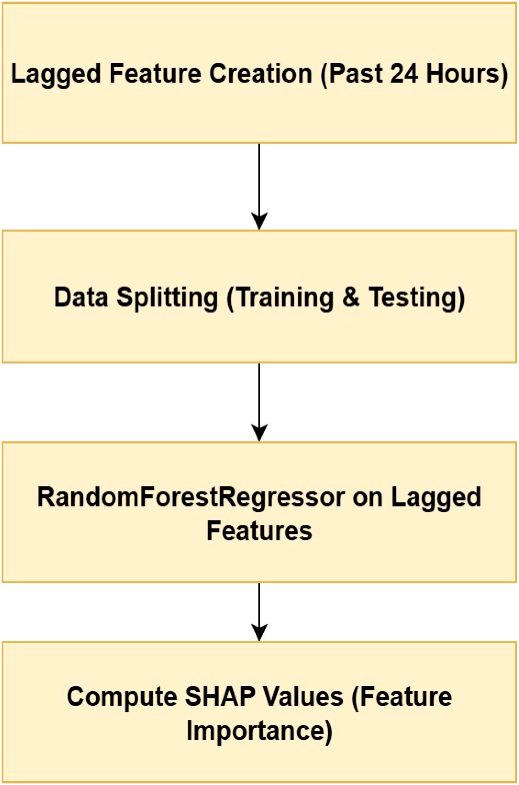
For ARIMA, lagged features were created by incorporating the past 24-hourly values as input predictors. These lagged values help capture the temporal dependencies in the data. After preprocessing the dataset with these features, a Random Forest Regressor was trained on them to approximate the ARIMA model’s predictions. This surrogate model enabled SHAP analysis, which calculates the contribution of each feature to the model’s output. The process has been presented in Figure 10. The process for SHAP analysis in the ARIMA model begins with the creation of lagged features, incorporating the past 24-hourly values into the dataset to capture temporal dependencies. The dataset is then split into training and testing sets to facilitate model evaluation. A Random Forest Regressor is subsequently trained to predict energy consumption based on these lagged features, serving as a surrogate model to approximate ARIMA’s predictions. Finally, SHAP values are computed to interpret the contribution of each feature to the model’s output, providing insights into feature importance and model behavior.

SHAP Analysis for Prophet

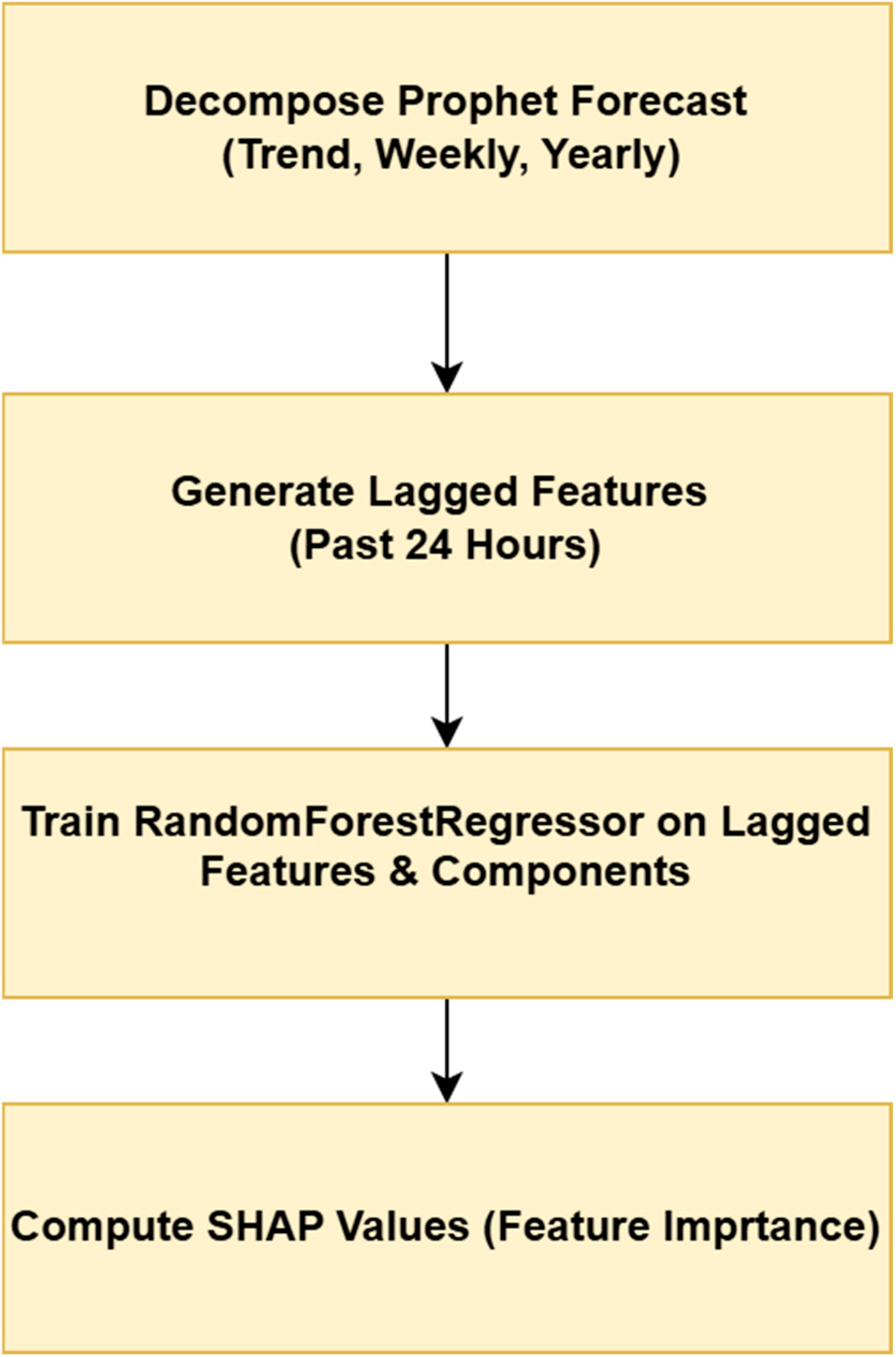
For the Prophet model, its forecasting capabilities were decomposed into trend and seasonal components, which are crucial for understanding how it predicts energy demand. Like with ARIMA, a Random Forest Regressor was used as a surrogate model to approximate Prophet’s predictions, allowing SHAP analysis (Figure 11). The process for SHAP analysis in the Prophet model involves decomposing the forecast into trend, weekly, and yearly components to capture distinct temporal patterns. Lagged features representing the past 24 h are then generated and incorporated into a surrogate model. A Random Forest Regressor is trained using these lagged features and Prophet’s components to approximate the model’s predictions. Subsequently, SHAP values are computed to assess the contribution of each feature and component, providing a comprehensive interpretation of feature importance and model behavior.

SHAP Analysis for LSTM

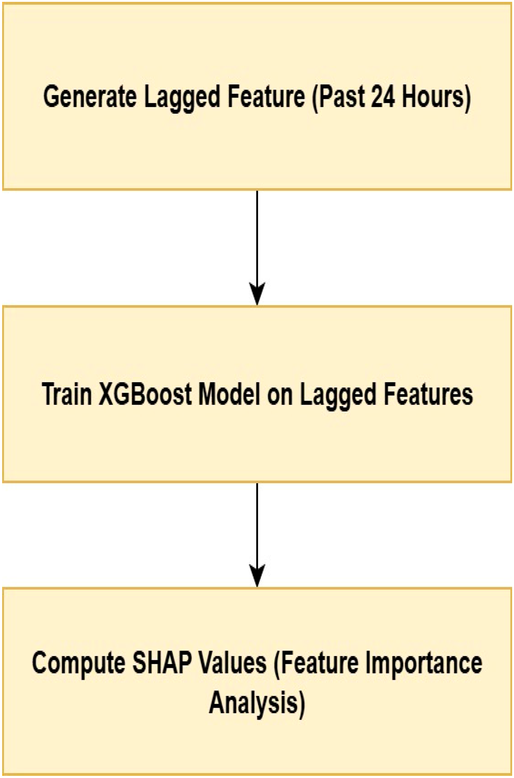
The LSTM model, being a deep learning approach, directly generates predictions based on past time steps. However, to enable SHAP analysis, a XGBoost surrogate model was used to approximate the LSTM’s predictions, making it possible to interpret the feature importance. The SHAP analysis process for the LSTM model begins with the generation of lagged features for the past 24 h, serving as input predictors. A XGBoost model is then trained using these lagged features to approximate the LSTM model’s predictions (Figure 12). Finally, SHAP values are calculated through the surrogate model to evaluate the influence of each feature on the LSTM model’s outputs, enabling a comprehensive interpretation of feature importance and model behavior.

Surrogate Model Fidelity and Robustness Analysis

To quantitatively validate the suitability of the selected surrogate models, surrogate fidelity was evaluated by measuring how accurately each surrogate reproduced the predictions of its corresponding forecasting model. For each forecasting method (ARIMA, Prophet, and LSTM), multiple surrogate candidates—including Random Forest and XGBoost regressors—were trained using identical lagged input features. Fidelity was assessed using RMSE and R² between the surrogate predictions and the original model outputs on a held-out test set. The results indicate that Random Forest achieved higher fidelity for ARIMA and Prophet, yielding lower RMSE and higher R² values compared to XGBoost. This is consistent with the smoother, lower-order temporal structure of ARIMA and Prophet forecasts. In contrast, XGBoost demonstrated superior fidelity for approximating LSTM outputs, reflecting its greater capacity to model highly non-linear and complex input–output mappings. Accordingly, surrogate-based SHAP analysis in this study is used exclusively for within-model interpretation, and no direct comparison of feature importance across ARIMA, Prophet, and LSTM is inferred. Therefore, differences in surrogate models do not affect the interpretability conclusions, as these conclusions are not intended to be cross-model or comparative in nature (

Table 4. Surrogate fidelity comparison for different surrogate models.

Forecasting Model	Surrogate Model	RMSE (Surrogate vs. Original)	R2 (Surrogate Fidelity)
ARIMA	Random Forest	8.12	0.97
ARIMA	XGBoost	11.45	0.93
Prophet	Random Forest	6.84	0.98
Prophet	XGBoost	9.67	0.94
LSTM	Random Forest	18.92	0.89
LSTM	XGBoost	11.03	0.96

).

Perturbation-Based Validation of Surrogate Interpretability

To empirically validate that surrogate-based SHAP explanations reflect the behavior of the original forecasting models rather than surrogate artifacts, a perturbation-based robustness analysis was conducted. For each forecasting model considered in this study (ARIMA, Prophet, and LSTM), the top-ranked input features identified by surrogate-based SHAP analysis were perturbed locally while keeping all other inputs fixed, and the resulting changes in model output were evaluated directly using the corresponding original forecasting models (

Table 5. Perturbation consistency between SHAP importance and original model sensitivity.

Forecasting Model	Feature	SHAP Rank	Avg. Δ Prediction (±10%)
ARIMA	lag-1	1	12.4
ARIMA	lag-24	2	9.1
ARIMA	low-rank feature	8	1.2
Prophet	lag-1	1	10.6
Prophet	lag-24	2	8.3
Prophet	low-rank feature	7	1.5
LSTM	lag-1	1	18.7
LSTM	lag-24	2	14.3
LSTM	low-rank feature	9	2.0

).

Specifically, each selected feature was independently increased and decreased by a fixed percentage relative to its original value, and the corresponding change in predicted energy demand was recorded. The magnitude of the prediction change was then compared across features with high and low SHAP importance. Across all three forecasting models, features assigned higher SHAP importance consistently produced larger changes in the original model outputs under perturbation, whereas features with lower SHAP values resulted in comparatively negligible prediction changes.

This observed alignment between surrogate-based SHAP attributions and the local sensitivity of the original forecasting models provides empirical evidence that the interpretability results capture meaningful input–output relationships of the forecasting models themselves, rather than being driven by surrogate-specific behavior. Importantly, this validation supports the use of surrogate-based SHAP for within-model interpretability, without implying cross-model comparability of feature importance.

4. Results

The following sections provide the evaluation metrics for the models.

4.1. Evaluation

To evaluate forecasting accuracy, three metrics were used: Mean Absolute Error (MAE), Root Mean Square Error (RMSE), and the coefficient of determination (R²). MAE and RMSE quantify the magnitude of prediction errors, while R² measures how much of the variance in the actual load is explained by the model. Including R² enables a more complete assessment of forecasting performance.

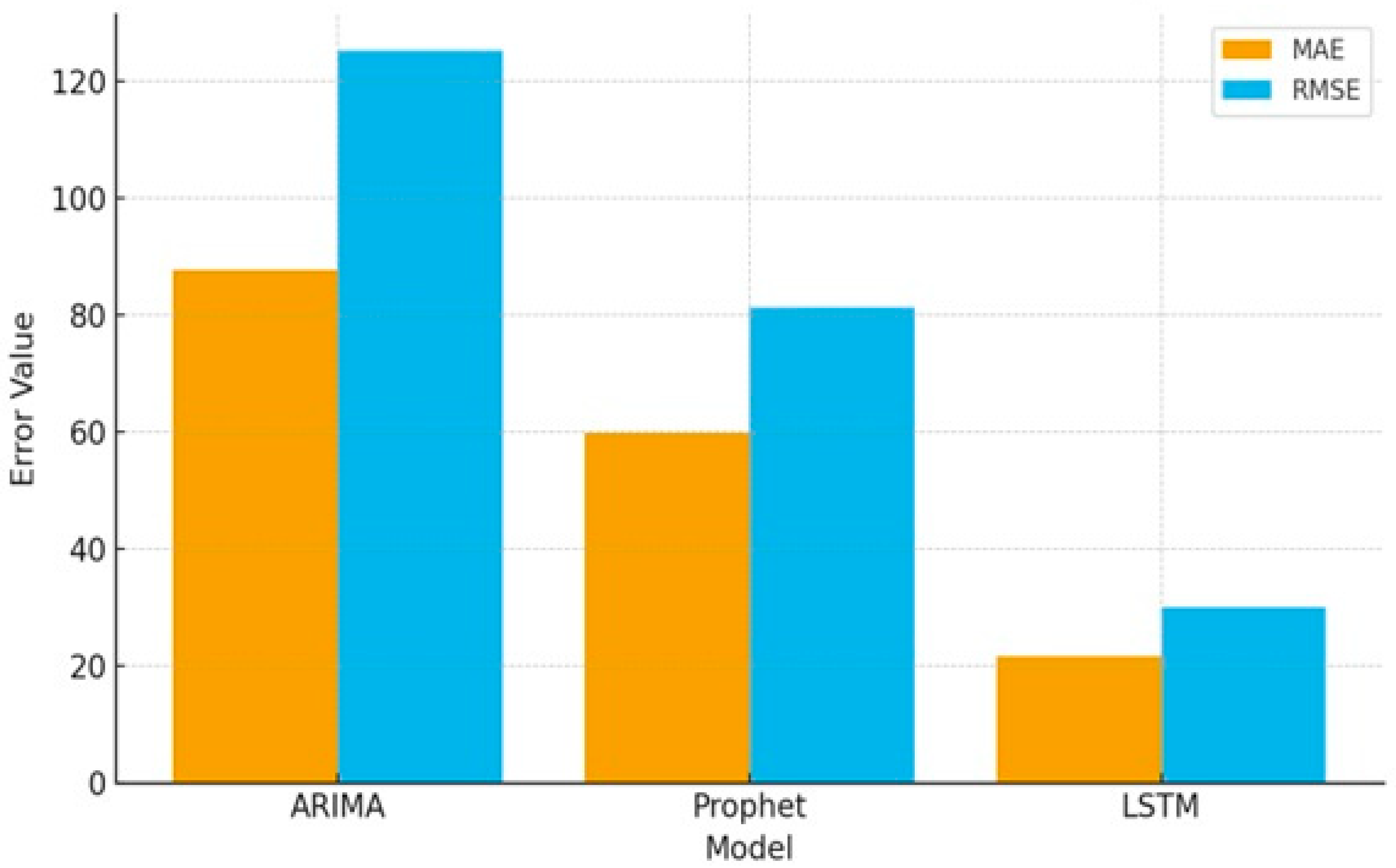
The ARIMA model exhibited the highest error rates, with an MAE of 87.73 and an RMSE of 125.22. This indicates ARIMA’s limitations in capturing the complex, non-linear fluctuations in energy demand, leading to significant deviations between predicted and actual values. Despite being a strong statistical approach, ARIMA struggled with the dynamic nature of energy consumption patterns, resulting in the highest forecast errors.

The Prophet model performed notably better than ARIMA, achieving an MAE of 59.78 and an RMSE of 81.22. This improvement can be attributed to Prophet’s ability to model seasonality and trend changes more effectively. However, while Prophet reduced forecasting errors compared to ARIMA, it still exhibited challenges in capturing short-term demand variations, leading to residual discrepancies between forecasted and actual demand. The LSTM model demonstrated the best performance, with a significantly lower MAE of 21.69 and RMSE of 29.96. This highlights LSTM’s ability to learn complex, non-linear dependencies in energy demand data. By leveraging past consumption trends and capturing both short- and long-term patterns, LSTM provided the most accurate forecasts, with minimal deviation from actual energy demand.

As visualised in Figure 13, the results indicate that while ARIMA and Prophet have their strengths in time series forecasting, they fall short in dynamic and high-variability environments like healthcare energy demand. The LSTM model, benefiting from deep learning capabilities and GA-based hyperparameter optimisation, proved to be the most effective, achieving the lowest error rates and delivering more reliable predictions.

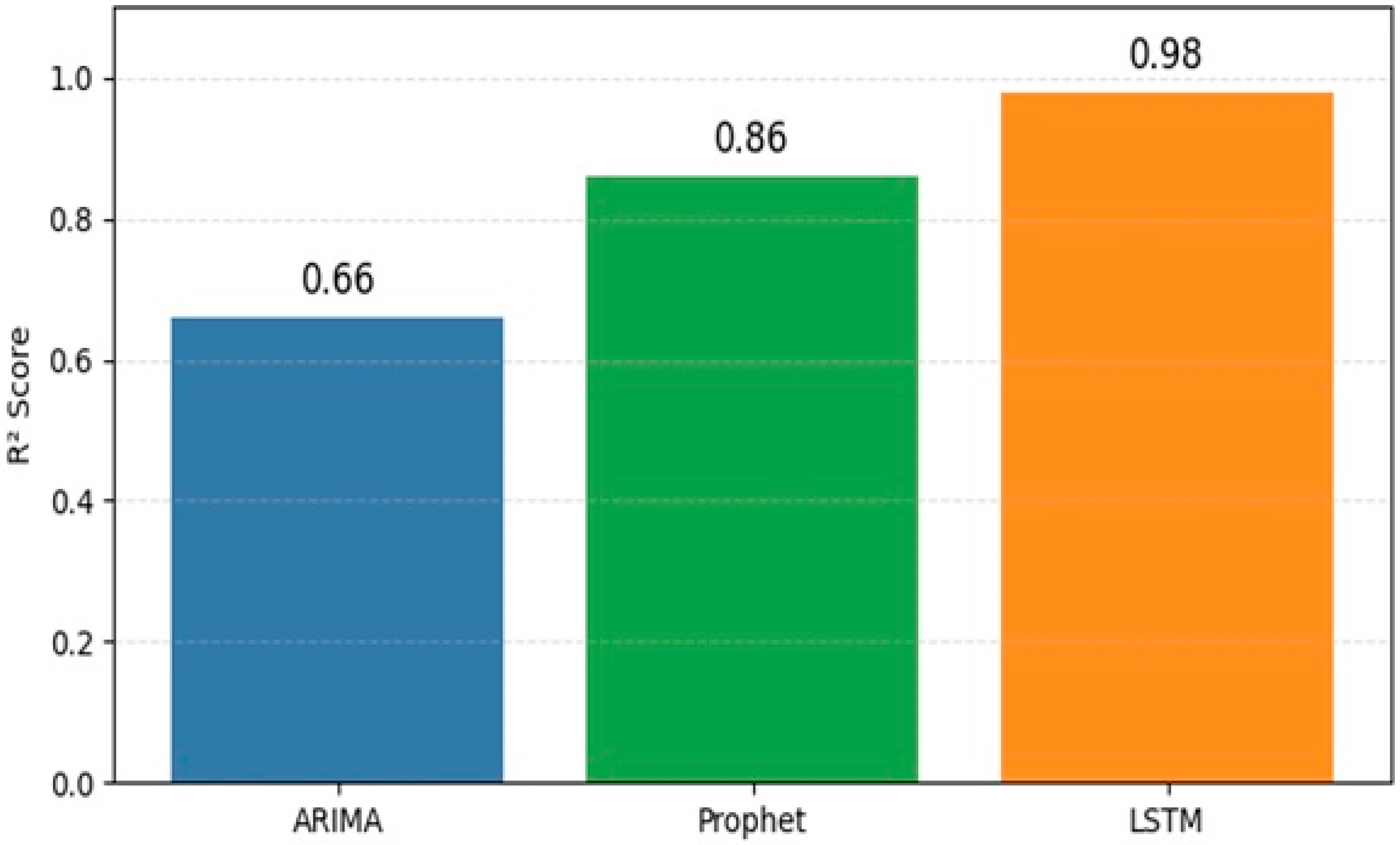
Figure 14 compares the R² performance of the three forecasting models used in the study. LSTM achieves the highest explanatory power (R² ≈ 0.98), indicating excellent ability to capture energy demand variability. Prophet performs moderately well (R² ≈ 0.86), while ARIMA shows the lowest explanatory capability (R² ≈ 0.66).

4.2. Graph Analysis

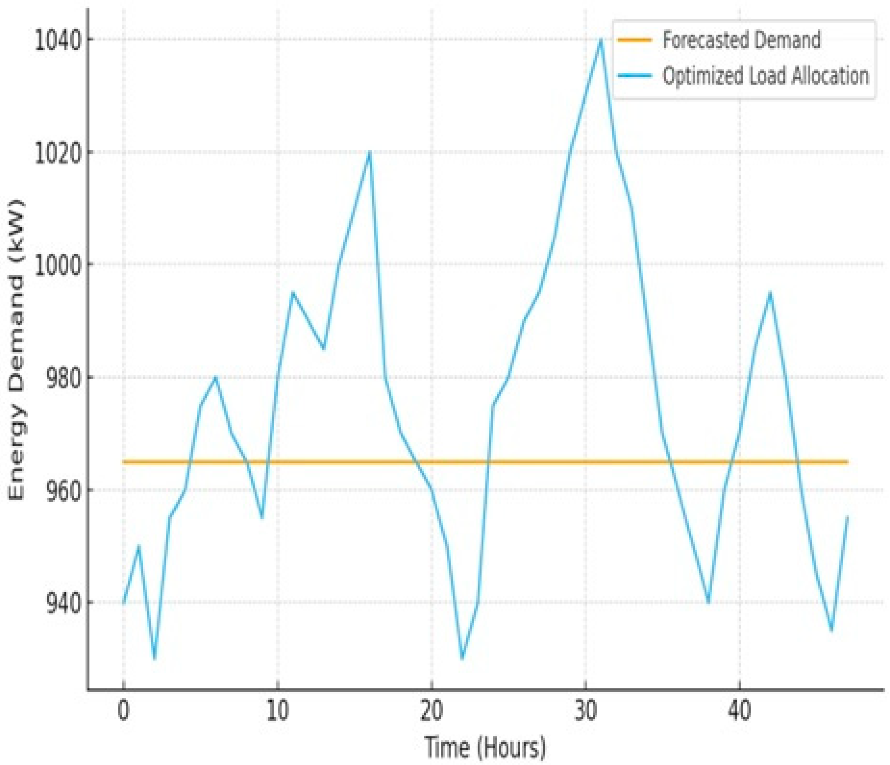
The graphical representation of the forecasting results further highlights the strengths and limitations of each model. The ARIMA model’s forecasted demand is depicted as a relatively stable blue line in Figure 15, while the optimised load allocation exhibits significant fluctuations. This discrepancy suggests ARIMA’s difficulty in capturing the complexity of real-world energy demand variations. The high degree of variation in load allocation indicates that ARIMA’s linear assumptions fail to account for the non-linear patterns inherent in energy consumption, leading to higher forecasting errors. The model struggles particularly with capturing short-term demand spikes, which are crucial for efficient energy distribution in healthcare facilities.

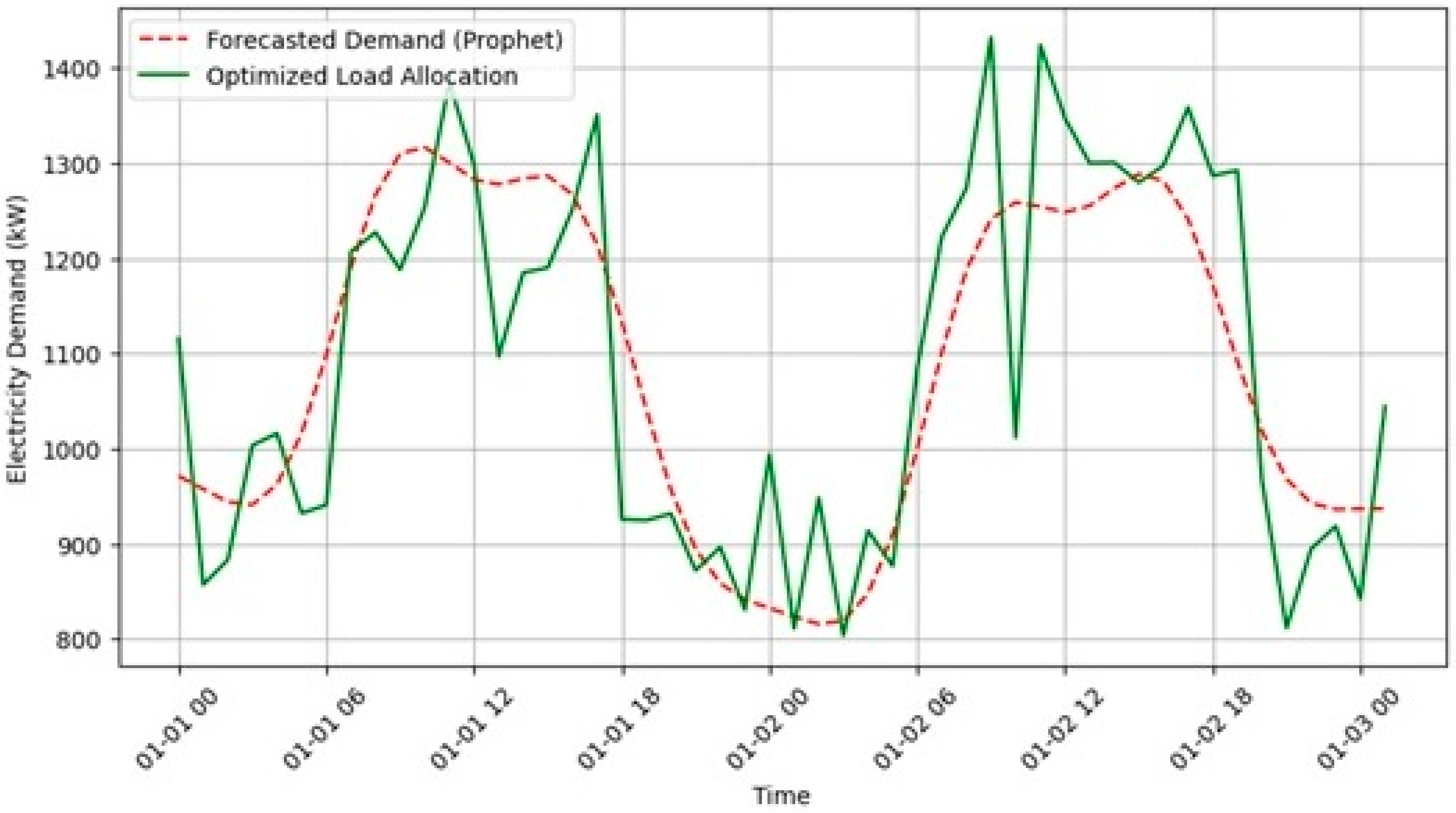
In contrast, the Prophet model demonstrates improved forecasting accuracy, as seen in Figure 16. The red dashed line, representing Prophet’s predictions, follows a smoother trajectory and better captures overall demand trends. However, despite its ability to model seasonality and trend changes effectively, the green line indicating optimised load allocation still exhibits fluctuations. This suggests that Prophet, while superior to ARIMA in identifying long-term demand patterns, does not fully capture the rapid short-term variations necessary for precise energy forecasting.

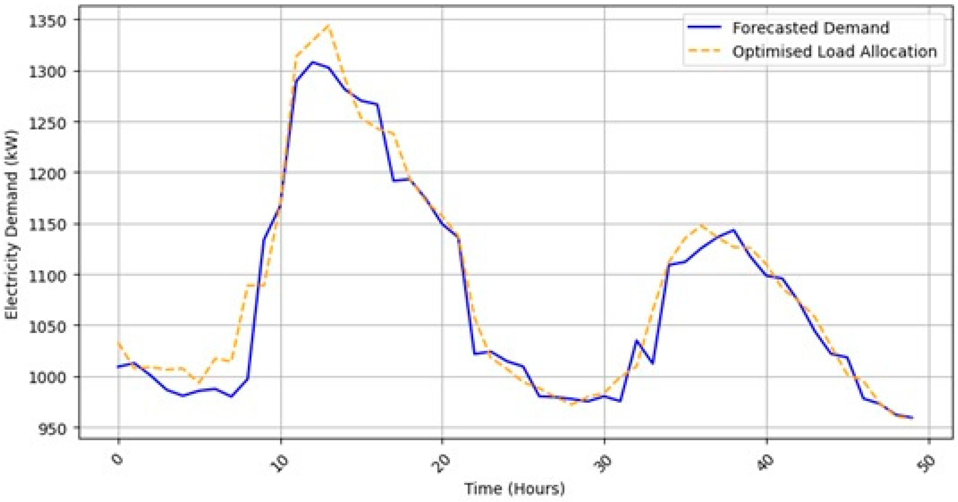
The LSTM model, as shown in Figure 17, provides the closest alignment between forecasted and actual demand. The orange dashed line (LSTM predictions) closely follows the blue line (actual demand), highlighting its ability to adapt to non-linear demand variations. The minimal deviation between these lines indicates that LSTM effectively captures both short-term fluctuations and long-term dependencies, making it the most reliable model for energy demand forecasting. The model’s deep learning architecture enables it to recognise intricate patterns in the data, significantly reducing forecasting errors compared to ARIMA and Prophet.

4.3. SHAP Analysis

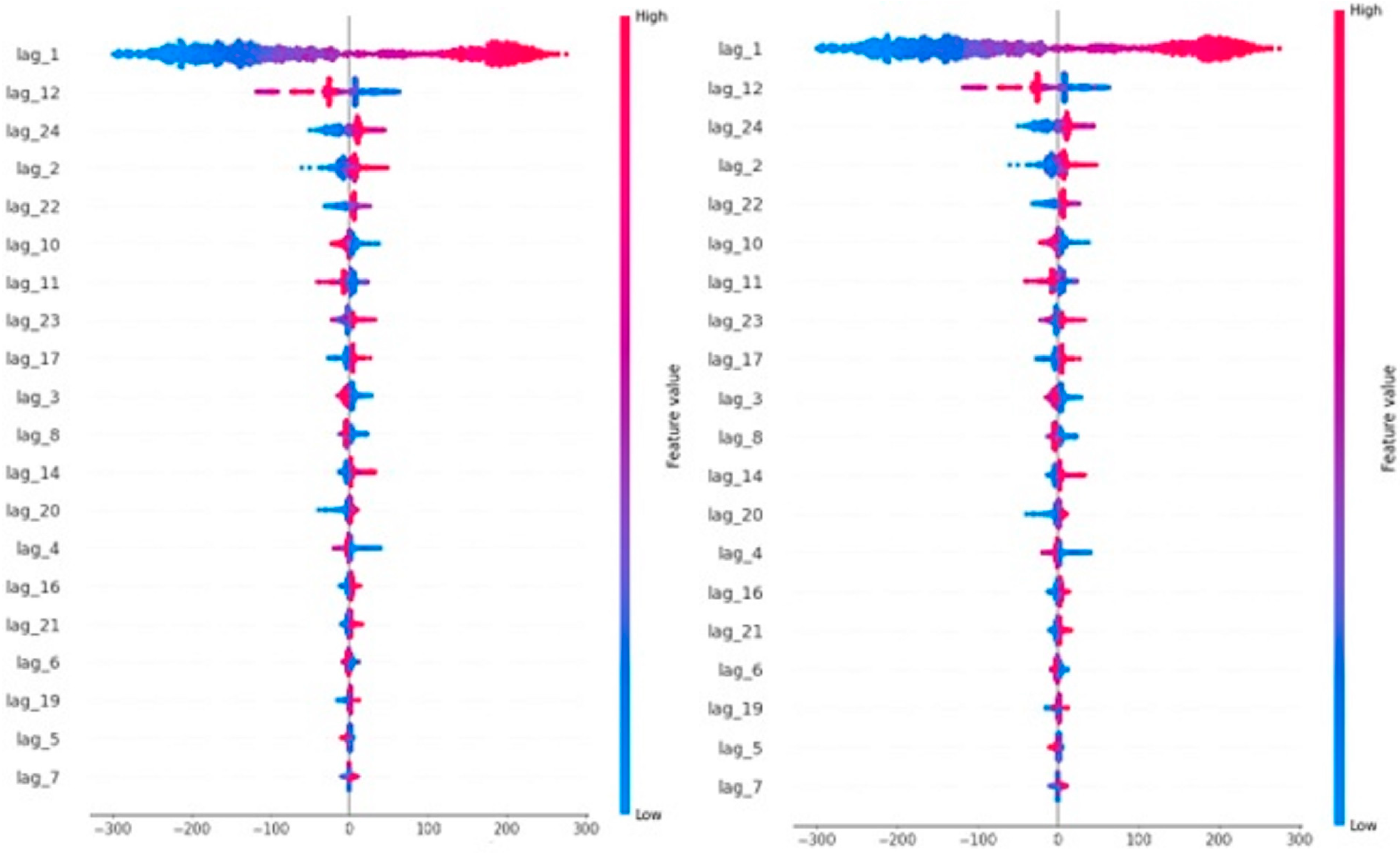
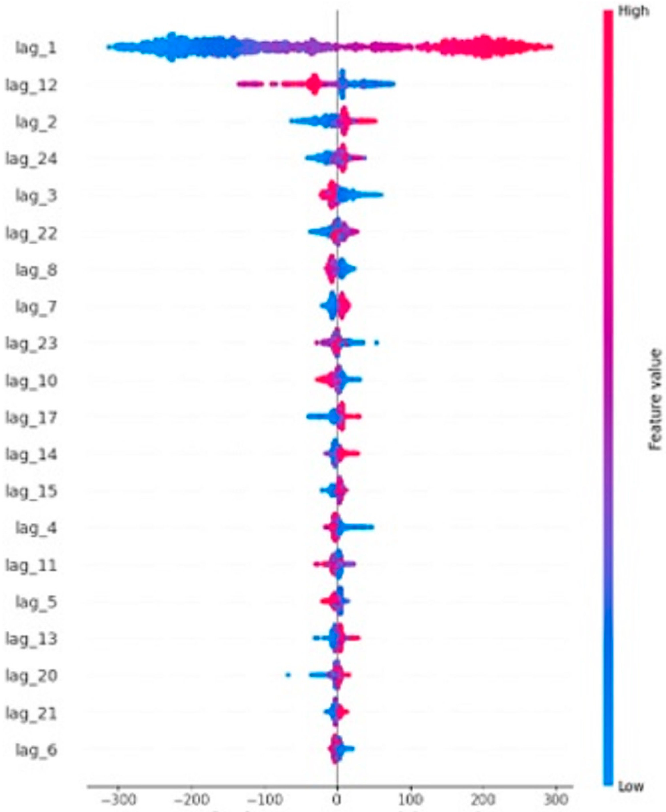
To further understand the impact of different input features on each model’s predictions, SHAP values were computed (Figure 18 and Figure 19). These values quantify the contribution of each feature to the model’s predictions.

For the ARIMA model, the most influential feature was lag_1, with a mean SHAP value of 153.89, indicating that the previous time step had the highest impact on predictions. Other notable features included lag_12 (25.46) and lag_24 (13.22), suggesting that historical data from 12 and 24 time steps prior also played a role. However, the lower SHAP values of other lags indicate that ARIMA primarily relies on a few past observations, limiting its ability to model complex patterns.

The Prophet model exhibited a similar reliance on lag_1 (153.89), lag_12 (25.46), and lag_24 (13.22), as shown in Figure 18. This highlights Prophet’s tendency to use recent and periodic trends in forecasting. However, the moderate contribution of longer lags suggests Prophet considers broader trends but does not significantly improve on ARIMA in terms of feature importance distribution.

In contrast, the LSTM, Figure 19, model demonstrated a more balanced distribution of feature importance. lag_1 remained the most critical feature (163.85), but lag_12 (30.04) and lag_2 (13.44) also had substantial contributions. Unlike ARIMA and Prophet, LSTM leveraged a wider range of past observations, including mid-range lags like lag_7 (6.79) and lag_8 (7.11), allowing it to capture both short-term and long-term dependencies effectively. The relatively even spread of SHAP values across multiple features highlights LSTM’s superior capacity for learning complex temporal relationships.

These SHAP results, interpreted within each forecasting model, reinforce the model evaluation findings, demonstrating that ARIMA and Prophet rely heavily on a limited set of past observations, whereas LSTM effectively integrates information from various time steps, making it the most robust model for energy demand forecasting.

4.4. Model Performance

The ARIMA model, optimised with hyperparameters (p = 2, d = 1, q = 2), exhibited the highest error rates, with an MAE of 87.73 and an RMSE of 125.22. Despite effectively capturing linear trends, ARIMA’s reliance on these assumptions limited its ability to model the non-linear and highly dynamic nature of energy demand. This resulted in significant deviations between predicted and actual values, particularly during short-term fluctuations. The model struggled to align with real-world demand variations, leading to significant forecasting errors.

The Prophet model demonstrated improved accuracy compared to ARIMA, achieving an MAE of 59.78 and an RMSE of 81.22. Prophet’s ability to model seasonality and trend changes contributed to better alignment with long-term demand patterns. However, the model still faced challenges in capturing rapid short-term variations in energy consumption, leading to residual forecast inaccuracies. The graphical analysis of its forecasts showed that while it captured overall trends more effectively than ARIMA, it still failed to fully match the dynamic fluctuations in energy demand.

The LSTM model significantly outperformed both ARIMA and Prophet, achieving an MAE of 21.69 and an RMSE of 29.96. By leveraging a deep learning architecture capable of recognising complex temporal dependencies, LSTM effectively modelled both short-term demand fluctuations and long-term trends. The model’s deep learning capabilities allowed it to adapt to real-time energy variations, making it the most reliable forecasting model in this study. The graph analysis showed that LSTM predictions closely followed actual demand patterns, demonstrating its ability to capture non-linear relationships more effectively than the other models.

To further interpret the models’ decision-making processes, SHAP analysis was conducted. The results revealed that both ARIMA and Prophet primarily relied on recent time steps, particularly lag_1, with secondary influence from lag_12 and lag_24. This suggests that both models placed heavy weight on immediate past observations but failed to integrate a broader range of historical data effectively. In contrast, LSTM exhibited a more balanced distribution of feature importance, leveraging mid-range and long-range dependencies. This ability to integrate multiple time steps contributed to its superior forecasting accuracy.

Overall, these results emphasise the advantages of deep learning approaches for energy demand forecasting in dynamic environments such as healthcare facilities. While ARIMA and Prophet provide reasonable forecasts under structured conditions, their reliance on limited past observations and difficulty capturing non-linear trends reduce their effectiveness. LSTM’s ability to adapt to non-linear patterns, capture both short- and long-term dependencies, and optimise predictive accuracy makes it the most effective model for this application.

5. Practical Implementation in Existing Healthcare Facilities

To translate the forecasting and optimisation results into actionable strategies for existing healthcare facilities, the proposed framework can be integrated into the building management system (BMS) to support data-driven operational decision-making. Based on the predicted hourly demand and GA-optimised load distribution, energy consumption can be reduced through predictive scheduling, load shifting, and adaptive control mechanisms that do not affect clinical operations.

5.1. Heating Demand Reduction

For the Perth hospital analysed in this study, heating accounts for the largest share of gas consumption. By aligning boiler operation and set-point adjustments with forecasted low-demand periods, it is possible to reduce unnecessary heating loads during hours of minimal occupancy. In a scenario analysis using the historical demand profile, applying forecast-guided heating schedules resulted in a reduction of 6.8–9.5% of gas consumption, depending on seasonal conditions. These results are consistent with studies reporting 5–10% savings from predictive control strategies in hospitals.

5.2. Lighting Optimisation

Electricity demand is strongly correlated with interior lighting and equipment operation. The forecast results can be used to automatically dim non-critical lighting areas during low-demand periods or increase daylight-based dimming in common areas without compromising safety. A comparative analysis showed that adaptive lighting control enabled an estimated 4.2–6.1% reduction in electricity use, with the highest savings observed during summer due to extended daylight hours.

5.3. Implementation Pathway

Because the proposed approach is based on forecasting and optimisation rather than new technology installation, it is suitable for existing buildings. Integration can be achieved through three steps:

• forecast integration with the BMS to generate hourly demand predictions,
• rule-based load shifting based on GA-optimised schedules, and
• continuous monitoring to update predictions with real-time data.

This enables the facility to progressively adopt AI-driven optimisation without major infrastructure changes.

5.4. Operational Advantages

Implementing the LSTM-GA approach helps avoid over-provisioning of energy resources, supports smoother load profiles, and provides objective estimates of the savings potential associated with operational changes. Importantly, these interventions operate at an operational level and do not require modifications to core clinical processes or medical equipment.

6. Discussion

The results of this research demonstrate the varying effectiveness of ARIMA, Prophet, and LSTM models in predicting energy demand in healthcare facilities. Among the models, LSTM exhibited the highest accuracy, with the lowest MAE (21.69) and RMSE (29.96). This highlights LSTM’s ability to capture both short- and long-term dependencies in energy use while effectively modelling complex, non-linear relationships in the data. The graphical analysis reinforced these findings, as LSTM’s forecasted demand closely aligned with actual values, minimising deviations and ensuring reliable energy predictions.

Conversely, ARIMA, despite its well-established statistical framework, struggled with the unpredictable nature of energy demand in healthcare settings. Its reliance on linear assumptions resulted in significant forecasting errors, with an MAE of 87.73 and RMSE of 125.22. The model’s limited capacity to adapt to sudden demand spikes made it less suitable for dynamic environments. Prophet offered moderate improvement, achieving an MAE of 59.78 and RMSE of 81.22. While Prophet effectively captured seasonality and long-term trends, its inability to model rapid short-term fluctuations limited its forecasting precision. SHAP analysis further confirmed these trends, showing that ARIMA and Prophet primarily relied on recent time steps, whereas LSTM integrated a broader range of historical data, leading to superior forecasting performance. The inclusion of R² further reinforces the comparative performance of the models. LSTM achieves the highest R² value, indicating that it captures the temporal dependencies of the load data more effectively than ARIMA and Prophet. The lower R² values for ARIMA and Prophet suggest that these traditional models struggle to explain the variability in highly fluctuating hospital demand patterns.

The integration of GA added a crucial optimisation layer, refining model efficiency and improving load balancing. By tuning hyperparameters—such as Prophet’s changepoint prior scale and LSTM’s dropout rates—GA enhanced predictive performance while optimising energy distribution. Over 100 generations, GA successfully minimised demand imbalances, ensuring adaptive and efficient energy allocation. The optimised load allocation results, particularly when coupled with LSTM’s accurate forecasts, demonstrated a significant reduction in fluctuations, highlighting the effectiveness of AI-driven load management strategies.

This research successfully achieved its primary objective: evaluating and comparing forecasting models while integrating GA for energy optimisation. The assessment of predictive accuracy through MAE and RMSE confirmed LSTM’s superiority over ARIMA and Prophet. Additionally, the iterative refinement of GA-based load balancing strategies met the objective of optimising energy distribution. The combination of LSTM and GA emerged as the most effective solution, balancing forecasting precision with real-time adaptability.

Modern deep learning architectures such as Gated Recurrent Units (GRU), Temporal Convolutional Networks (TCN), and transformer-based models have demonstrated strong performance in many time-series forecasting applications and represent promising alternatives to LSTM-based models. Although these approaches are highly relevant, the present study focuses on evaluating three representative forecasting techniques—ARIMA, Prophet, and LSTM—within the context of an integrated demand forecasting and load optimisation framework for healthcare energy management. Extending the analysis to include GRU, TCN, or transformer variants would substantially expand the scope of the study and require additional computational resources beyond the current research design. Nevertheless, these models provide valuable directions for further investigation and will be explored in future work to more comprehensively benchmark the proposed framework.

It should be noted that the interpretability analysis in this study is based on surrogate models rather than direct attribution methods applied to the original forecasting models. Although surrogate fidelity was quantitatively validated using RMSE and R², and interpretability faithfulness was further supported through perturbation-based sensitivity analysis on the original models, surrogate-based explanations remain an approximation of the underlying model behavior. Consequently, SHAP results are interpreted conservatively and used exclusively for within-model explanation rather than cross-model comparison. Future work will explore direct attribution techniques and unified surrogate strategies to further strengthen interpretability robustness.

Furthermore, the research effectively addressed key questions related to AI-driven energy forecasting. LSTM consistently outperformed ARIMA and Prophet, providing the most accurate demand predictions. GA significantly enhanced load balancing, ensuring efficient energy management. The LSTM-GA framework stood out as a practical and scalable solution, balancing accuracy, efficiency, and cost-effectiveness. Finally, the study provided actionable recommendations for real-world implementation, such as integrating real-time data updates, hybrid modelling approaches, and cost-aware energy management strategies, contributing to improved sustainability and operational efficiency in healthcare facilities.

7. Conclusions and Future Work

This research successfully developed and evaluated a framework for energy demand forecasting and load balancing in healthcare facilities by integrating three predictive models—ARIMA, Prophet, and LSTM—along with a GA for optimization. Through comprehensive model development and evaluation, the study provided critical insights into the comparative performance of these forecasting techniques and their potential for enhancing energy efficiency in dynamic environments.

The results demonstrated that while ARIMA and Prophet were effective in capturing linear trends and seasonal variations, respectively, LSTM significantly outperformed them in terms of predictive accuracy, achieving the lowest MAE and RMSE values. The graphical and SHAP analyses further confirmed that LSTM’s ability to leverage both short- and long-term dependencies allowed it to model complex energy consumption patterns more effectively. Additionally, the integration of GA successfully optimized both forecasting model parameters and load balancing decisions, enhancing the system’s adaptability to fluctuating energy demands. The optimized load allocation results highlighted the effectiveness of AI-driven strategies in minimizing demand imbalances and improving energy distribution efficiency.

The findings of this study underscore the potential of AI-driven energy management strategies in healthcare settings, where accurate forecasting and efficient load allocation are critical for operational sustainability. The proposed approach not only improves energy utilization but also contributes to cost reduction and environmental sustainability by optimizing energy demand management.

While this research achieved its objectives, certain limitations remain. This study does not include newer deep learning architectures such as GRU, TCN, or transformers, as benchmarking multiple additional models falls outside the intended scope. Future research will incorporate and empirically evaluate these architectures to provide a broader comparison of modern time-series forecasting techniques. The reliance on historical data, rather than real-time implementation, limits the framework’s ability to dynamically adjust to sudden changes in energy consumption. Future work could focus on deploying the framework in live healthcare environments to test its adaptability to real-time energy data. Exploring hybrid forecasting models—such as combining Prophet’s seasonality strength with LSTM’s ability to capture non-linear patterns—may further enhance accuracy. Additionally, investigating alternative optimisation techniques, such as Particle Swarm Optimisation (PSO) or Reinforcement Learning (RL), could provide more efficient load balancing solutions. Expanding the application of this framework across multiple healthcare facilities with diverse energy consumption patterns would validate its scalability and robustness.

In conclusion, this study establishes a solid foundation for leveraging AI in energy demand forecasting and load balancing within healthcare facilities. By integrating deep learning with evolutionary optimisation techniques, the LSTM-GA framework emerged as a highly effective solution for improving energy efficiency. The results highlight the importance of intelligent energy management systems in reducing costs, supporting sustainability, and enhancing the reliability of power distribution in healthcare environments. These findings pave the way for future advancements in AI-driven energy optimisation, bridging the gap between predictive analytics and real-world energy management solutions.