Fault Detection and Diagnosis of Rolling Bearings in Automated Container Terminals Using Time–Frequency Domain Filters and CNN-KAN

Abstract

In automated container terminals (ACTs), rolling bearings of equipment serve as crucial power transmission components, and their performance directly determines the operational efficiency, reliability, and service life of the entire equipment. Rolling bearing fault detection and diagnosis are key means to improve production efficiency, reduce the safety risks, and achieve sustainable development of equipment in ACTs. However, existing rolling-bearing diagnosis models are vulnerable to environmental noise and interference, depressing accuracy and raising misclassification, and they seldom achieve both noise robustness and a lightweight design; robustness usually increases complexity, while compact networks degrade under low signal-to-noise ratios. Therefore, this paper proposes a noise-robust, lightweight, and interpretable deep learning framework for fault detection and diagnosis of rolling bearings in automated container terminal (ACT) equipment. The framework comprises four coordinated components, including Time-Domain Filter, Frequency-Domain Filter, Physical-Feature Extraction module, and Classification module, whose joint optimization yields complementary time–frequency representations and physics-aligned features, and fuses into robust diagnostic decisions under noisy and non-stationary environments. The first component highlights impulsive transients, the second component emphasizes harmonic and sideband modulation, the third module introduces two differentiable and rolling bearing-signal-informed objectives to align learning with characteristic bearing signatures by weighted-average kurtosis and an Lp/Lq-based envelope-spectral concentration index, and the last module integrates multi-layer convolutional neural networks (CNN) and Deep Kolmogorov–Arnold Networks (DeepKAN). Finally, two public datasets are employed to estimate the model’s performance, and results indicate that the proposed method outperforms others.

1. Introduction

As a strategic node of national key infrastructure and global supply chain, the value of ports has expanded from traditional cargo distribution functions to the core engine of regional economic development [1]. Automated Container Terminals (ACTs), as a typical paradigm of port modernization, has built an intelligent control system for the entire container operation chain through the integration of artificial intelligence, Internet of Things, and automation control systems. In this system, intelligent equipment, such as automated quay cranes, yard cranes, and automated guided vehicles (AGVs), serve as key production equipment shown in Figure 1, and their technical performance directly characterizes the operational level and service quality of ACTs, which is the technological cornerstone for shaping the core competitiveness of ports. Specifically, as the core functional component of the power transmission system, the dynamic characteristics and reliability indicators of rolling bearings of equipment in ACTs fundamentally determine the operational efficiency, stability, and service life of the equipment system.

The key equipment in ACTs faces dual challenges of extreme working conditions in long-term operation: (1) this equipment has to withstand high-intensity continuous operations under outdoor environments, (2) it encounters multiple problems, such as component wear and ageing, impact loads during cargo handling, and corrosion from marine climate. All of these factors interact with each other, significantly increasing the risk of equipment faults, especially because rolling bearings of equipment in ACTs are prone to failure under the dual effects of continuous high-intensity operation and long-term harsh marine environments. If not detected and handled in a timely manner, it will not only cause operational interruptions, but also significantly increase maintenance costs.

To effectively address this challenge, ACTs commonly apply sensor networks to build equipment health management systems in intelligent construction. Real-time monitoring of operational status can be achieved by deploying multiple types of sensing devices at critical locations. However, the complex operational environment in ACTs leads to serious noise interference in the detected data, including mechanical vibration noise of the equipment itself, surge impact noise unique to marine environments, and high-frequency electromagnetic interference generated by electrical systems. These noises are deeply coupled with effective signals, resulting in high false alarm rates for traditional fault detection methods under strong interference environments. Specifically, rolling bearing fault signals are characterized by periodic impact impulses and exhibit second-order cyclostationarity; during propagation, they are distorted by transfer paths and become embedded in strong non-stationary noise. The most diagnostic information appears as discrete characteristic lines in the envelope spectrum, which may drift around nominal values, while the response remains sparse in both time and frequency. Moreover, deep learning models engineered for strong noise robustness often incur substantial computational cost in the form of large parameter counts and high FLOPs, which hinders edge deployment in ACTs. In addition, conventional architectures offer limited interpretability grounded in vibration-domain features, such as characteristic fault frequencies and their modulation sidebands, making it difficult to trace diagnostic decisions to the underlying physical mechanisms.

To address this problem, a novel deep learning framework named the time–frequency and physical feature extraction network (TFPNet) is proposed for rolling bearings of equipment in ACTs under noisy environments. Unlike conventional CNN-based approaches and hybrid wavelet-CNN methods that frequently encounter challenges related to limited noise suppression capability and high computational complexity, the proposed TFPNet innovatively integrates advanced time–frequency domain filters with physical feature extraction methods, significantly enhancing fault diagnostic accuracy, noise resilience and computational efficiency. The main contributions of this paper are summarized as follows:

• We propose a deep learning fault detection and diagnosis framework for rolling bearings of equipment in ACTs, comprising Time-Domain Filter, Frequency-Domain Filter, Physical Feature Extraction, and Classification Module. The framework is designed to address poor performance of fault diagnosis models from noise interference while preserving a lightweight architecture.
• A Physical Feature Extraction module incorporates weighted average kurtosis and $L_p/L_q$ norm to construct a physics-informed prior loss. The former one captures impulsive characteristics to distinguish fault-related impulses from random noise, and the latter one enhances the contrast between characteristic frequencies and broadband noise. This loss is jointly optimized with the classifier’s cross-entropy loss that focuses learning on fault-discriminating signal components and bridges physical interpretability with data-driven optimization.
• CNN and DeepKAN are incorporated to jointly model temporal patterns and complex nonlinear features to enhance the ability to distinguish faults, addressing the impact of non-stationary and noise interference on fault diagnosis.

The rest of the paper is organized as follows. Section 2 reviews related work. Section 3 illustrates our methodology. Section 4 validates the effectiveness of the proposed framework by two public datasets. Section 5 concludes this paper.

2. Related Work

In this Section, we will review the literature on fault detection and diagnosis from the perspectives of traditional mechanical equipment and port equipment.

2.1. Fault Detection and Diagnosis of Mechanical Equipment

As the core foundation of industrial production and agricultural activities, the stable operation of equipment is directly related to production efficiency and economic benefits. With the rapid development of Industry 4.0 and intelligent manufacturing technologies, fault detection and diagnosis technologies of mechanical equipment is undergoing revolutionary changes. Traditional methods based on threshold detection and spectrum analysis are no longer sufficient to meet the diagnostic needs of modern, complex working conditions, especially under specialized environments, such as open-air ports and mines, where the operational status of monitoring equipment faces numerous challenges.

In response to these challenges, intelligent diagnostic methods based on deep learning have demonstrated significant advantages. For instance, Hong et al. [2] proposed a modular neural network for fault detection and classification of semiconductor manufacturing equipment. Wang et al. [3] designed a fault diagnosis method based on back propagation neural network for complex electronic equipment. Zheng et al. [4] applied YOLOv4 for target detection and rapid extraction of equipment temperature, achieving intelligent diagnosis of thermal faults in substation power equipment. Mendonça et al. [5] used Fuzzy Logic theory to detect and diagnose faults in ship equipment. Muzzammel et al. [6] presented a fault analysis and classification method for three source transmission lines, in which values of instantaneous power and signed power are used for fault detection and classification, and voltage curves are used to identify fault locations. Prince et al. [7] proposed an improved hybrid 1D convolutional neural network for fault detection and diagnosis of an Air-Handling Unit. Amiri et al. [8] integrated CNN and Bi-GRU for fault detection and diagnosis of a photovoltaic system. Li et al. [9] proposed a migration learning method based on adaptive batch normalization for rotating machinery fault diagnosis.

The monitoring signals of mechanical equipment are often severely affected by noise interference, which greatly affects the accuracy and reliability of fault diagnosis models. However, traditional denoising techniques are difficult to effectively handle non-stationary signals and complex noise. For instance, methods based on time–frequency analysis, such as wavelet transform [10] and empirical mode decomposition [11], have been widely used due to their computational efficiency advantages, but they are not suitable for data containing non-stationary noise and signals. With the rapid development of deep learning technology, intelligent denoising methods based on neural networks have shown significant advantages in the field of mechanical fault diagnosis. For example, Peng et al. [12] innovatively proposed a two-stage framework that integrates denoising sparse autoencoders and smooth integral gradients, which not only effectively eliminated noise interference but also enhanced the interpretability of fault diagnosis results. Zhong et al. [13] further developed an attention guided parallel convolutional neural network, achieving collaborative optimization of noise suppression and fault diagnosis. Kim et al. [14] developed a fast response anomaly detection system for industrial noise environments by combining deep denoising autoencoders with unsupervised learning strategies. These studies collectively indicate that efficient denoising has become key to improving the fault detection accuracy and diagnostic reliability of mechanical equipment. Existing denoising methods underuse the time–frequency characteristics of industrial noise and often lack domain-specific physical priors, which hampers reliable separation of noise and fault features in noise-intensive settings. At the same time, balancing strong noise robustness with a lightweight design remains difficult: highly robust models typically require large parameter counts and high FLOPs, whereas lightweight architectures often degrade at low signal-to-noise ratios. The current research trend tends to integrate physical prior knowledge with deep learning models, further improving noise suppression performance while maintaining computational efficiency.

2.2. Fault Detection and Diagnosis of Port Equipment

Fault detection and diagnosis of port equipment are crucial tasks in port equipment management and can often be achieved through some machine learning or deep learning methods to extract complex features of faults. For instance, Ding et al. [15] considered the uncertain status of AGV and proposed a fault detection method based on Decision Tree and Long Short-Term Memory (LSTM) for AGV equipment, fully leveraging the advantages of Decision Tree in rule learning and LSTM in the extraction of hidden features. Tian et al. [16] considered the multi-source heterogeneous operation and maintenance data of loading and unloading equipment in dry bulk ports, advanced a feature fusion deep learning model to extract features of structured and unstructured data, and then the fused feature vectors were used to achieve fault detection for loading and unloading equipment. Meanwhile, some researchers employ mechanical vibration or acoustic emission to analyze the characteristic frequency components of different faults and then identify mechanical damage [17]. For example, Van Steen et al. [18] adopted Wavelet Transform to conduct mechanical vibration analysis in fault diagnosis, Seleznev et al. [19] introduced acoustic emission technology to identify micro-damage and crack formation.

Moreover, troubleshooting and predicting port equipment faults have become important means of port equipment management because they can recognize potential problems in advance, avoid faults, and reduce downtime and maintenance costs. Sensor devices installed on port equipment are used to collect data for potential fault risk analysis and prediction by intelligent technologies. For example. Yoon et al. [20] presented a wireless sensing system for structural health monitoring of harbor caisson structures, which monitored and forecasted damage to critical port equipment structures. Chaibi and Daghrir [21] employed artificial intelligence to identify trends, patterns, and early signs of faults from port equipment status, enabling proactive planning and maintenance. Halim and Tang [22] proposed a graphical method to obtain the confidence interval of the optimal preventive maintenance (PM) interval generated by sampling variation parameter estimation and calculated the sampling risk faced by the PM interval. Although existing fault-diagnosis techniques have made progress, when applied to rolling bearings in ACT equipment the strong electromagnetic interference and structure-borne vibrations of port operations often bury fault signatures, significantly reducing diagnostic accuracy and reliability. In practice, solutions must also deliver real-time performance on widely distributed edge devices through lightweight designs, and there is a need for physics-aligned interpretability to establish decision trust beyond black-box deep learning. Therefore, a noise-robust, lightweight, and interpretable fault-diagnosis framework for rolling bearings in ACT equipment is of great practical significance.

3. Methodology

Vibration signals of rolling bearing in ACTs exhibit multi-scale impulsive components, pronounced non-stationarity, and low signal-to-noise ratios. These properties motivate a design that preserves long-range temporal dependencies under noisy environments, enhances localized band-limited transients across scales, and imposes physics-grounded regularization to stabilize learning and maintain interpretability. Inspired by the property alignment, we propose a universal fault detection and diagnosis framework based on a Time–Frequency and Physical Feature Extraction Network (TFPnet) for rolling bearings of equipment in ACTs, which comprises four cooperating modules as shown in Figure 2, including a Time-Domain Filter, a Frequency-Domain Filter, a Physical Feature Extraction block, and a Classification module.

Specifically, The Time-Domain Filter employs depthwise-separable convolution and attention to suppress noise and aggregate long-range dependencies, forming a temporal scaffold that stabilizes subsequent spectral weighting. The Frequency-Domain Filter applies fast Fourier transform (FFT), multi-level wavelet decomposition, and convolution for multi-resolution spectral analysis. The fused spectral representation is mapped back to the time domain via inverse FFT (IFFT) to achieve shape alignment and enable joint optimization with the temporal stream. The Physical Feature Extraction block computes weighted-average kurtosis and the $L_p/L_q$ ratio in the view of both time and frequency domains, and introduces them as auxiliary losses optionally with dynamic weighting to co-regularize both streams toward impulsive and spectrally concentrated patterns, improving stability and interpretability. Finally, the Classification module integrates multi-layer CNNs and DeepKAN to optimize the fused time–frequency embedding under these constraints. This task-driven, tightly coupled framework yields progressive refinement of discriminative structure and robust diagnosis under noisy, non-stationary conditions, while maintaining a lightweight architecture and providing physics-aligned interpretability.

3.1. Time-Domain Filter

The Time-Domain Filter integrates four sub-modules to accomplish tasks ranging from local nonlinear enhancement to global periodic dependency capture for enhancing the noise resistance performance of fault detection and diagnosis models. These sub-modules include Quadratic Convolution (QConv), Depthwise Separable Convolution (DSConv), a Linear Attention mechanism (LinearAttn), and a Multi-layer Perceptron (MLP), whose structure is illustrated in Figure 3, and the function of each sub-module will be described in detail below.

A.

Quadratic Convolution

Based on the nonlinear expression ability of quadratic neurons, QConv constructs three sets of convolutional channels to model the linear response, inter channel modulation, and squared enhancement term in the signal, thereby breaking through the limitations of single order convolution on complex feature modeling. The output format of QConv is defined as follows.

$$H_1=\left({Conv1D}_r\right(X)+b_r)\odot \left({Conv1D}_g\right(X)+bg)+{Conv1D}_b\left(X^2\right)+b_b$$

(1)

where $X$ is the input feature, ${Conv}_r$, ${Conv}_g$, ${Conv}_b$ are three one-dimensional convolution operations, respectively. $b_r, b_g, b_b$ are the corresponding bias terms. $\odot$ represents Hadamard product, and $X^2$ represents the square of each element.

QConv can effectively extract local high-order statistical characteristics from vibration signals pf rolling bearings, and its weight separation strategy can further enhance the model’s noise resistance. QConv can be used as a high-order local modeling method with explicit second-order polynomial expression ability, suitable for capturing the impact response and instantaneous energy changes in early fault signals of rolling bearings [23].

B.

Depthwise-Separable Convolution

While QConv highlights impulsive onsets via explicit second-order locality, vibrations of rolling bearings also contain weak, drifted quasi-periodic harmonics beyond purely local modeling. Therefore, this Section appends a depthwise-separable stage to provide phase-aware, wider context for these band-limited periodic structures.

Although DSConv has the advantage of feature extraction, its receptive field is limited without introducing explicit position information, making it difficult to capture temporal dependencies and weak impact displacements accurately. Therefore, this Section introduces Convolutional Positional Encoding (CPE) based on one-dimensional deep convolution, expressed as Equation (2).

$${H_1}^{\prime }={CPE(H}_1+DWConv1D\left(H_1\right))$$

(2)

where $DWConv1D$ is a one-dimensional deep convolution. On the basis of preserving local information features, this model considers temporal and positional information to enhance the perceptual ability of subsequent convolutions, effectively improving the modeling ability of subsequent DSConv for shocks and disturbances. DSConv consists of two parts, namely $DWConv1D$ and Pointwise Convolution ($PWConv1D$) [24]. The former independently extracts local features within the channel, while the latter completes inter channel fusion and has good noise resistance performance, whose definition is given in Equation (3).

$$H_2=PWConv1D\left(DWConv1D\left(H_1^{\prime }\right)\right)$$

(3)

CPE and DSConv are arranged in series, which endows DSConv with explicit temporal–positional awareness during local feature extraction. Compared with conventional stacks or simple convolution concatenations, this configuration is well suited to conditions with periodic or phase drift and weak impulsive components. At the same time, the depthwise-separable kernels markedly reduce parameter count and FLOPs, yielding a lightweight, low-latency module suitable for edge deployment.

C.

LinearAttention

Because DSConv is essentially a local feature model and is limited in capturing long-range temporal dependencies, this Section introduces a linear attention mechanism as a complementary global modeling module. Combining locally position-enhanced features with globally dynamic attention enables joint perception and fused modeling of local and global information, thereby improving the recognition of complex periodically modulated impact signals and enhancing overall modeling performance.

For rolling-bearing vibration signals that are typically high-frequency, long-sequence, low-SNR, and contain weak periodic impulses, conventional softmax attention suffers from quadratic time complexity ($O\left(N^2\right)$), sensitivity to high-amplitude noise, and limited generalization. Standard linear-attention variants reduce complexity but do not account for the nonlinear structure and local modal characteristics specific to bearing signals, which restricts their ability to capture weak fault features. To address these issues, we propose a globally perception-enhanced linear-attention mechanism tailored to bearing diagnosis; through a nonlinear kernel mapping and an optimized scheme for global feature aggregation, it efficiently models long-range dependencies, markedly strengthens noise robustness, and maintains linear complexity with a lightweight footprint.

The nonlinear kernel function ELU is first used to map the query ($Q$) and key ($K$) to enhance the ability of expressing weak periodic perturbations and nonlinear changes. The negative smoothing of ELU can suppress high-frequency noise interference. $Q$, $K$ and value vector ($V$) are defined as Equations (4)–(6).

$$Q=ELU\left(W_Q{H}_2\right)$$

(4)

$$K=ELU\left(W_K{H}_2\right)$$

(5)

$$V=W_V{H}_2$$

(6)

where $W_Q$, $W_K$ and $W_V$ are learnable projection matrixes.

Then, the computational cost is reduced, and numerical stability is enhanced by using a global aggregation strategy to avoid positional interaction calculations. The global representation tensor $S$ and normalization factor $Z$ are calculated as follows:

$$S=\sum _{j=1}^N{K}_j^T{V}_j$$

(7)

$$Z=\sum _{j=1}^N{K}_j^T$$

(8)

where $K_j^T$ and $V_j$ represent the key and value vectors at the jth position in the sequence, respectively. This method aggregates key–value information across all positions in a single pass, avoiding per-position interactions and reducing computational complexity from $O\left(N^2\right)$ to $O\left(N\right)$, which makes it well suited for lightweight global modeling of long bearing vibration sequences. Subsequently, the attention output of the ith position is shown as Equation (9).

$$H_3^{\left(i\right)}={\displaystyle \frac{Q_i\cdot S}{Q_i\cdot Z+\epsilon }}$$

(9)

where $\epsilon$ is a small constant term that prevents zero division.

A residual branch is designed in global linear attention to further enhance the feature adaptability of the model on one-dimensional bearing vibration sequences.

Through SiLU nonlinear activation, a time-varying gate vector $G$ is obtained, and then the $H_3^{\left(i\right)}$ is multiplied by $G$ to obtain gate features, and $H_1^{\prime }$ is added to form the final feature. This reduces the amplification effect of high-frequency noise on the attention output while maintaining linear computational complexity in the network, which is defined as Equation (10)

$$H_3=H_3^{\left(i\right)}\odot G+{H_1}^{\prime }$$

(10)

Overall, the LinearAttn has good modeling effect and engineering adaptability for typical fault signals of rolling bearings, such as high-frequency impact, low signal-to-noise ratio, and periodic drift.

D.

Multi-layer Perceptron

To enhance the nonlinear modeling capacity of high-dimensional features for fault signals of rolling bearings, we design a compact and efficient multi-layer perceptron (MLP) that operates downstream of the linear attention module as a feature-enhancement block. MLP consists of two linear mappings and a GELU activation function, with a Dropout layer inserted in between to improve generalization performance. MLP is defined as Equation (11).

$$H_4=W_2\cdot \mathrm{D}\mathrm{r}\mathrm{o}\mathrm{p}\mathrm{o}\mathrm{u}\mathrm{t}\left(GELU\left(W_1{H}_3+b_1\right)\right)+b_2$$

(11)

where $W$ is the weight matrix, $b$ is the bias term.

Unlike conventional time-domain modules, the proposed Time-Domain Filter introduces a hierarchical design tailored to impulsive, non-stationary signals of rolling bearing. QConv explicitly models second-order nonlinearities for high-order impulse detection, DSConv with CPE enhances position-aware periodic perception under phase drift, and a noise-robust LinearAttn captures global dependencies with linear complexity while suppressing high-frequency bursts via gated residuals. Together with a lightweight MLP, these modules form a complementary framework that significantly improves denoising robustness and interpretability, providing a stable representation basis for subsequent frequency-domain enhancement and physics-informed loss design.

3.2. Frequency-Domain Filter

After undergoing the preliminary suppression of impulsive noise and local non-stationary disturbances by the Time-Domain Filter, vibration signals of rolling bearings still contain a large number of frequency-dominated interference components. These interferences not only mask the real fault frequency characteristics but also reduce the discriminative ability and generalization performance of the diagnosis models. To further extract physically meaningful key frequency components and enhance the robustness of frequency-domain features, this Section designs the Frequency-Domain Filter module as a supplementary modeling structure after time-domain processing.

The Frequency-Domain Filter converts $H_4$ to frequency domain through Fast Fourier Transform (FFT), which is defined as Equation (12).

$$X_{freq}=FFT\left(H_4\right)$$

(12)

The Frequency-Domain Filter adopts a dual-branch modeling strategy consisting of a basic spectral path and a wavelet path, which is responsible for capturing global spectral structures and local frequency disturbances, respectively, to extract discriminative spectral features. The architecture of this module is illustrated in Figure 4.

The basic spectral path applies one-dimensional convolution to the amplitude spectrum, as in Equation (13), to extract the spectral energy distribution and its variations, and to identify stable frequency patterns that serve as global references, while maintaining a low parameter budget.

$$Y_{base}=Conv1D\left(X_{freq}\right)$$

(13)

The wavelet path focuses on modeling local non-stationary disturbances in the frequency spectrum, whose structure is given in Figure 3. To meet the input length requirements of discrete wavelet transform, padding is applied to the original frequency domain signal, and the filled signal serves as the initial value of the low-frequency sub-band $X_{LL}^{\left(0\right)}$ in the 0th layer, which is defined as Equations (14) and (15).

$$X_{pad}=Padding\left(X_{freq}\right)$$

(14)

$$X_{LL}^{\left(0\right)}=X_{pad}$$

(15)

Subsequently, a wavelet decomposition operation is recursively performed on the low-frequency sub-band $X_{LL}^{\left(i-1\right)}$ of each layer to generate the low-frequency sub-band $X_{LL}^{\left(i\right)}$ and high-frequency sub-band $X_{LH}^{\left(i\right)}$, which are used to capture multi-scale frequency features.

$$X_{LL}^{\left(i\right)},X_{LH}^{\left(i\right)}=WT\left(X_{LL}^{\left(i-1\right)}\right)$$

(16)

Meanwhile, the multi-level decomposition halves the sequence length at each level, yielding a geometrically decreasing FLOPs profile and a reduced memory footprint, thereby enabling a lightweight frequency-domain branch suitable for edge deployment.

In order to further extract effective local structural features, one-dimensional Wavelet convolutions [25] are applied to each sub-band layer to obtain feature representations.

$$F_s^{\left(i\right)}=Conv1D\left(X_s^{\left(i\right)}\right)\hspace{1em}\hspace{1em}\hspace{1em}\mathrm{s}\mathsf{ϵ}\{LL,LH\}$$

(17)

where $F_{LL}^{\left(i\right)}$ represents the result of low-frequency sub-band convolution and emphasizes the global trend, $F_{LH}^{\left(i\right)}$ is the result of high-frequency sub-band convolution and extracts local perturbations. By introducing a channel weighting mechanism namely Wavelet Attention and assigning a learnable scaling factor Scale to each channel, key frequency bands are enhanced through global weighting defined as Equation (18). Channel-wise scaling introduces one learnable gain per channel and only performs element-wise rescaling along the sequence, so both the parameter count and the additional runtime cost remain small.

$$F_{att}^{\left(i\right)}=Scale\left(F_{LL}^{\left(i\right)}+F_{LH}^{\left(i\right)}\right)$$

(18)

where $F_{att}^{\left(i\right)}$ is the result of channel weighting. The weighted multi-scale sub-band feature $F_{att}^{\left(i\right)}$ is subjected to inverse wavelet transform (IWT) from top to bottom, and frequency domain reconstruction is performed layer by layer, which is defined as follows.

$$Z^{(i-1)}=IWT(Z^{\left(i\right)}+F_{att}^{\left(i-1\right)}) \mathrm{i}=1, 2,\dots , L$$

(19)

where $Z^{\left(L\right)}=F_{att}^{\left(L\right)}$. By using multi-level inverse wavelet transform, the lowest reconstruction result $Z^{\left(0\right)}$ is restored to match the shape of the filled signal $X_{pad}$, and the output is the enhanced feature $Y_{wavelet}=Z^{\left(0\right)}$. During the reconstruction process, both the global trend information in the low-frequency sub-band and the local detail response in the high-frequency sub-band are retained, improving the modeling ability for weak frequency disturbances in fault features. A complete frequency domain representation is obtained by fusing the results of wavelet path and basic spectral path.

$$Y_{final}=Y_{base}+Y_{wavelet}$$

(20)

To achieve a closed-loop feature transformation from frequency domain to time domain, this Section further introduces inverse fast Fourier transform (IFFT) to map the fusion result $Y_{final}$ back to the time domain space as Y, which facilitates collaborative optimization with subsequent time domain feature extraction or physical constraint mechanisms.

Designed around the vibration intrinsic characteristics of rolling bearings, including cyclostationarity, amplitude and phase modulation, and weak order-related lines under noise, the innovations of the Frequency-Domain Filter lie in its task-driven architecture for signals of rolling bearings. Specifically, a dual-path firstly design combines a spectral branch for global harmonic trends with a wavelet branch for local non-stationary perturbations, enhanced by wavelet attention with adaptive scaling. Then, an IFFT-based time–frequency loop maps fused spectral features back to the time domain, ensuring that frequency-domain enhancements directly benefit impulsive feature recognition and mitigating the traditional disconnection between separated time- and frequency-domain processing. Moreover, a recursive multi-layer WT/IWT scheme progressively integrates high-frequency sub-band details into lower layers, preserving global structures while alleviating detail loss in weak-signal scenarios. Overall, these designs enable robust extraction of both stable characteristic frequencies and transient modulations under strong noise conditions, while maintaining a lightweight, low-latency implementation.

3.3. Physical Feature Extraction Based on Weighted Average Kurtosis and $L_p/L_q$ Norm

In this Section, we propose a physical feature extraction method that combines weighted average kurtosis and $L_p/L_q$ norm [26] to address the difficulty in accurately extracting fault features of rolling bearings under strong noise environments. Specifically, the weighted average kurtosis is employed to perform weighted statistical analysis on the time-domain filter output, strengthening the high variance impact areas related to faults. The $L_p/L_q$ norm ratio is adopted to reflect the concentration of energy at the fault characteristic frequency in the envelope spectrum, effectively highlighting the periodic modulation components caused by bearing faults.

A.

Weighted Average Kurtosis

Faults of rolling bearings may generate periodic impulsive signals, which manifest as distinct peaks in the time domain and thus result in an elevated kurtosis value. In contrast, random noise exhibits no periodicity and corresponds to a lower kurtosis value. Consequently, kurtosis can effectively discriminate between fault-related impulses and noise. But the traditional kurtosis index is usually highly sensitive to a single or a few abnormal noise points, which can easily lead to local pseudo peaks, thereby reducing the ability to accurately identify the impact of real faults. To alleviate this problem, this paper proposes a Weighted Average Kurtosis (WAK) algorithm to enhance the expressive ability and robustness of local impact features under strong noise environments. The WAK divides the input signal $H_4=\{{H_4}_1,{H_4}_2,{H_4}_3\dots \dots {H_4}_n\}$ into multiple sub-segments of equal magnitude M, calculates the kurtosis value ${kurtosis}_i$ of each segment separately, and normalizes the weight $w_i$ based on the corresponding variance ${\sigma }_i^2$.

$${kurtosis}_i={\displaystyle \frac{\frac{1}{n}{\sum }_{i=1}^n{({H_4}_i-\mu )}^4}{{\left(\frac{1}{n}{\sum }_{i=1}^n{{(H_4}_i-\mu )}^2\right)}^2}}$$

(21)

$$w_i={\displaystyle \frac{{\sigma }_i^2}{{\sum }_{k=1}^M{\sigma }_k^2}}$$

(22)

$$a_k=\sum _{i=1}^M{w}_i\cdot {kurtosis}_i$$

(23)

where $\mu$ represents the mean, $ak$ represents the weighted average kurtosis, ${\sigma }_i^2$ is the variance of the i-th segment signal, ${\sigma }_k^2$ is the variance of the k-th segment, and k is a cyclic variable from 1 to $M$.

This weighting strategy can amplify the contribution of regions with high information density to global kurtosis, thereby enhancing the response strength of impact features and suppressing the risk of misjudgment caused by local high amplitude noise.

B.

$L_p/L_q$ Norm

Due to the modulation characteristics of rolling bearing fault, their envelope spectra exhibit sparsity, with energy concentrated at discrete characteristic frequencies, while broadband noise tends to distribute energy diffusely. By combining different sensitivity properties of $L_p/L_q$ norms, the $L_p/L_q$ ratio amplifies the contrast between concentrated spectral peaks and dispersed noise components, thereby suppressing broadband interference and highlighting fault-related frequencies. To further improve robustness under low signal-to-noise ratio conditions, this paper develops an envelope feature modeling method based on the $L_p/L_q$ norm ratio. The method enhances the characterization ability of energy concentrated periodic components in fault signals.

This Section first introduces an IFFT to map the fusion result $Y_{final}$ back to the time-domain signal $Y$. The Hilbert transform is then applied to $Y$ to construct the analytic signal and extract its envelope after removing the DC component. Subsequently, a Fourier transform is performed on the envelope, and the resulting spectrum is denoted as $Fenv\left(f\right)$. To suppress high-frequency noise pseudo peaks and enhance the expression of feature frequencies, the energy weighting factor is introduced as follows.

$$E(f)={\displaystyle \frac{2\cdot \mid Fenv\left(f\right)\mid }{N+ϵ}}$$

(24)

where $N$ is the signal length, and $ϵ$ is a small constant to prevent numerical instability. This weighting factor constrains excessive energy accumulation of high-frequency noise, reducing the likelihood of noise-induced pseudo peaks and thereby improving the discriminability of fault characteristic frequencies in $Fenv\left(f\right)$). Subsequently, the $L_p/L_q$ norm ratio index is constructed, which exhibits a greater response when the energy concentration of periodic shock components is concentrated, helping to enhance the detection ability of weak features. It is defined as follows:

$$g=log({\displaystyle \frac{(Nor{m}_q{)}^q}{(Nor{m}_p{)}^p+ϵ}})$$

(25)

$$p=\mathit{log}\left(1+e^{{logp}_{raw}}\right)+1.0$$

(26)

$$q=log(1+e^{{logq}_{raw}})+1.0$$

(27)

where $Nor{m}_q$ and $Nor{m}_p$ represent the p-norm and q-norm of the envelope signal, and $ϵ$ is the stable term to prevent gradient explosion or disappearance, and the Softplus function is introduced for positive normalization of $p$ and $q$. The adaptive adjustment of $p$ and $q$ via the Softplus function is tailored to the sparsity of fault characteristic frequencies, where the energy is concentrated at discrete frequency points. When $p$ < $q$, the criterion enhances sensitivity to periodic components, which is consistent with the monotonicity of the generalized sparsity measure.

Meanwhile, two physics-guided auxiliary losses are embedded into the end-to-end objective. The WAK loss, evaluated on the Time-Domain Filter output, amplifies impact-rich segments while suppressing noise. The $L_p/L_q$ loss, computed from the envelope spectrum derived by the Frequency-Domain Filter, promotes spectral energy concentration at characteristic lines and sidebands. Because both losses are differentiable, their gradients backpropagate through the Time-Domain Filter and the Frequency-Domain Filter, forming a closed time–frequency learning loop that strengthens robustness and interpretability under non-stationary, low-SNR conditions.

In summary, the envelope analysis method proposed in this article can effectively characterize the energy accumulation characteristics exhibited by periodic shocks in the envelope spectrum, improving the sensitivity and robustness of fault identification under complex operating conditions.

3.4. Classification Module Based on CNN and DeepKAN

In response to the strong non-stationarity and noise interference characteristics in fault signals of rolling bearings, this Section presents the design of a classification module that integrates multi-layer convolutional neural networks (CNN) and DeepKAN, aiming to achieve fine-grained modeling of high-dimensional nonlinear features and high robustness fault classification, whose structure is shown in Figure 5.

Specifically, the model first receives the enhanced features output by the previous Time-Domain Filter and Frequency-Domain Filter, and constructs a four layer one-dimensional convolutional backbone network to extract features. This network uses progressively decreasing convolutional kernels, with the earlier layers capturing long-term periodic patterns using larger receptive fields, while the later layers focus on short-term shocks and local disturbance features through small-scale convolution. To compress data dimensions, reduce redundant information, and suppress overfitting, pooling layers are introduced after each convolutional layer to preserve discriminative multi-scale structural information.

To enhance nonlinear modeling capability and improve noise stability, this paper introduces a DeepKAN module composed of multiple KAN Blocks after CNN feature extraction. This module is based on the Kolmogorov–Arnold representation theorem, which decomposes high-dimensional complex mappings into weighted combinations of single variable learnable functions. By learning the shape of the activation function to adapt to local disturbances and nonlinear structures of the signal, the modeling ability of the model for periodic modulation and impulse characteristics is improved. Compared to the traditional MLP fixed nonlinear activation method, DeepKAN has higher feature modeling flexibility and parameter efficiency.

Each KAN Block contains KAN Layer, DWConv, Batch Norm, and ReLU activation. KAN Layer achieves flexible nonlinear mapping through the combination of univariate functions. DWConv performs independent convolution operations along the channel dimension to enhance the KAN layer’s ability to capture feature details. Batch normalization and ReLU activation function improve training stability and nonlinear processing capability.

Among them, the KAN activation function is constructed by combining the basic nonlinear mapping $b\left(z\right)$ with B spline to form an adaptive activation function, and its calculation form is defined as Equation (28).

$$\Phi (z)=w_{1}b\left(z\right)+w_{2}spline\left(z\right)$$

(28)

$$b(z)=\mathrm{SiLU}(z)={\displaystyle \frac{z}{1+e^{-z}}}$$

(29)

$$\mathit{spline}(z)=\sum _i{c}_i{B}_i(z)$$

(30)

where z is input vector, the $spline\left(z\right)$ is a learnable activation part weighted by the B spline basis function $B_i\left(z\right)$, coefficient $c_i$ is the training adjustable parameter, $w_1$ and $w_2$ are the amplitude adjustment coefficient of the activation function. Through adaptive optimization of $c_i$, $w_1$ and $w_2$ during the training process, the KAN layer can dynamically learn the shape of the activation function, achieving accurate approximation of complex nonlinear functions.

The Deep KAN module can refine the high-dimensional features output by the CNN encoder layer-by-layer, enhancing the model’s ability to recognize key fault patterns, such as periodic disturbances and transient impacts, thereby improving the diagnostic accuracy and robustness of bearing fault types under strong noise conditions.

In addition, to enhance the physical interpretability of the model, a multi-task optimization objective combining physical loss and cross-entropy loss are designed as follows.

$$l_{\mathit{a}\mathit{v}\mathit{g}\_\mathit{w}\mathit{t}\mathit{e}\mathit{d}\_\mathit{k}\mathit{u}\mathit{r}\mathit{t}\mathit{o}\mathit{s}\mathit{i}\mathit{s}}=-{\displaystyle \frac{1}{N^{\prime }}}\sum _{n=1}^N{a}_k^{\left(n\right)}$$

(31)

$$l_{\mathit{e}\mathit{n}\mathit{v}\mathit{e}\mathit{l}\mathit{o}\mathit{p}\mathit{e}}=-{\displaystyle \frac{1}{N^{\prime }}}\sum _{n=1}^N{g}^{\left(n\right)}$$

(32)

where $N^{\prime }$ is the batch size, $a_k^{\left(n\right)}$ is the weighted average kurtosis of the nth sample, $g^{\left(n\right)}$ is the $L_{p/}{L}_q$ norm ratio of the nth sample. $l_{\mathit{a}\mathit{v}\mathit{g}\_\mathit{w}\mathit{t}\mathit{e}\mathit{d}\_\mathit{k}\mathit{u}\mathit{r}\mathit{t}\mathit{o}\mathit{s}\mathit{i}\mathit{s}}$ and $l_{\mathit{e}\mathit{n}\mathit{v}\mathit{e}\mathit{l}\mathit{o}\mathit{p}\mathit{e}}$ are two loss functions of weighted average kurtosis and $L_{p/}{L}_q$ norm, which enhance the sensitivity of capturing impulsive faults and periodic shocks.

$${l_{total}=l_{time-frequency}+{\lambda }_{1}l}_{\mathit{a}\mathit{v}\mathit{g}\_\mathit{w}\mathit{t}\mathit{e}\mathit{d}\_\mathit{k}\mathit{u}\mathit{r}\mathit{t}\mathit{o}\mathit{s}\mathit{i}\mathit{s}}+{\lambda }_2 l_{\mathit{e}\mathit{n}\mathit{v}\mathit{e}\mathit{l}\mathit{o}\mathit{p}\mathit{e}}$$

(33)

$l_{total}$ is the ultimate goal of model optimization by combining classification tasks and physical constraints. $l_{time-frequency}$ is a cross-entropy loss based on time–frequency fusion features. Exponential moving average (EMA) is used to estimate the losses of various physical loss terms, while parameter adjusted Softmax function is utilized for dynamic weight allocation. This strategy aims to adaptively balance the contribution of each physical loss term to the total loss, ensuring its improvement in training stability during multi-task optimization.

Different from the fixed nonlinear activation of traditional CNN-MLP classifiers, this study proposes a learnable spline activation function based on DeepKAN to achieve adaptive approximation of nonlinear mappings. This method enhances feature extraction capability under noisy environments by parameterizing spline basis functions, and explicitly embeds domain knowledge by combining physical constraints, such as weighted average kurtosis loss and $L_p/L_q$ norm ratio. This data-driven and physically guided framework improves fault detection performance and model robustness.

4. Experiment and Discussion

In this Section, we employ publicly available datasets to validate the effectiveness of the methods proposed earlier and discuss them.

4.1. Datasets

In order to fully verify the generalization of the proposed method, experiments were conducted using the bearing dataset from Harbin Institute of Technology [27] and the bearing fault dataset from Jiangnan University [28].

A.

The Bearing Dataset of Harbin Institute of Technology (HIT)

The engine used in the test bench of this dataset retains a dual rotor structure (low-pressure/high-pressure compressor and turbine) and key bearings, with six sensors installed: two displacement sensors (low-pressure rotor) and four acceleration sensors (casing). The test was conducted under 28 sets of high/low pressure speed combinations (speed range 1000–6000 rpm) with a sampling frequency of 25 kHz. The collected data included acceleration vibration signals and displacement vibration signals of the low pressure rotor, totaling 2412 sets of data. Each set was a truncated segment of the 15 s vibration signal with 20,480 data points.

Manufacturing faults (depth 0.5 mm, length 0.5/1.0 mm) in the inner/outer ring of the intermediate bearing through wire cutting, simulating the periodic impact of real faults. This dataset contains four types of labels, including one bearing with outer ring fault, two bearings with inner ring fault, and healthy bearings. The detailed information on the bearings is shown in

Table 1. Bearing information.

Bearings	Fault Type	Fault Depth/mm	Fault Length/mm	Fault Label
A	No Fault	0	0	0
B	Out Ring Fault	0.5	0.5	1
C	Inner Ring Fault	0.5	0.5	2
D	Inner Ring Fault	0.5	1	3

.

B.

The Bearing Dataset of Jiangnan University (JNU)

The bearing fault dataset of Jiangnan University has a sampling frequency of 50 kHz and contains four types: normal state, inner ring fault, outer ring fault, and rolling element fault. During the experiment, an accelerometer was used to collect vibration signals at three different speeds of 600, 800, and 1000 r/min. Therefore, under different working conditions, the total number of rolling bearing categories is 12. In this study, the sliding window method is used to segment each sample into 2048 fixed length data points. As a result, a total of 89,850 samples were extracted, with a total of 183,091,200 data points.

4.2. Data Preparation and Evaluation

To improve the generalization ability and robustness of the model under strong noise environments, the data preprocessing in this article includes multiple steps, such as sample segmentation, noise injection, and data augmentation.

The original vibration signal is divided into fixed length segments for subsequent modeling. The duration of a single channel acceleration signal is 15 s, with a sampling rate of 25 kHz. This article divides data into structured sub-sample sequences using a sliding window with a length of 2048 points. All sub-samples are divided into datasets based on the original samples, and training, validation, and testing sets are constructed in proportions of 70%, 20%, and 10%, respectively, to ensure that all windows of the same original sample do not span multiple sub-sets, effectively avoiding data leakage issues.

By adding Gaussian white noise of different intensities as model input to the raw data samples, the vibration signal fault diagnosis in actual noisy environments is simulated. The signal-to-noise ratio (SNR) is usually chosen as an important indicator to evaluate the intensity of noise, and the calculation is given in Equation (34).

$$SNR=10\mathrm{l}\mathrm{g}\left({\displaystyle \frac{p_s}{p_n}}\right)$$

(34)

where $p_s$ and $p_n$ are the power of the original signal and the noise signal. The smaller the signal-to-noise ratio, the stronger the noise. When the signal-to-noise ratio is less than 0 dB, it is a strong noise environment, and the power of the noise signal is greater than that of the original signal. The signal-to-noise ratio range in the experiment was set to −8 to 0 dB. Subsequently, a data augmentation strategy was applied to the data, and the window signal was randomly scaled to enhance the robustness of the model to signal strength changes. Fifteen percent of the frequency band was randomly masked in the frequency domain to simulate the actual situation of missing frequency components.

The performance of the proposed method is evaluated by commonly used evaluation indicators, including Accuracy (Acc), false positive rate (FPR), Recall, Precision, and F₁ score. The FPR represents the proportion of individuals who are actually “healthy” but incorrectly identified as “faulty” by the model. Equation (39) defines the balance between the Precision and Recall of fault types in the F₁ comprehensive reflection model.

$$Acc={\displaystyle \frac{TP+TN}{TP+TN+FP+FN}}$$

(35)

$$FPR={\displaystyle \frac{FP}{FP+TN}}$$

(36)

$$Recall={\displaystyle \frac{TP}{TP+FN}}$$

(37)

$$Precision={\displaystyle \frac{TP}{TP+FP}}$$

(38)

$$F_1={\displaystyle \frac{2\times Recall\times Precision}{Recall+Precision}}$$

(39)

where TP, TN, FP, and FN represent the number of true positives, true negatives, false positives, and false negatives, respectively.

4.3. Results and Discussion

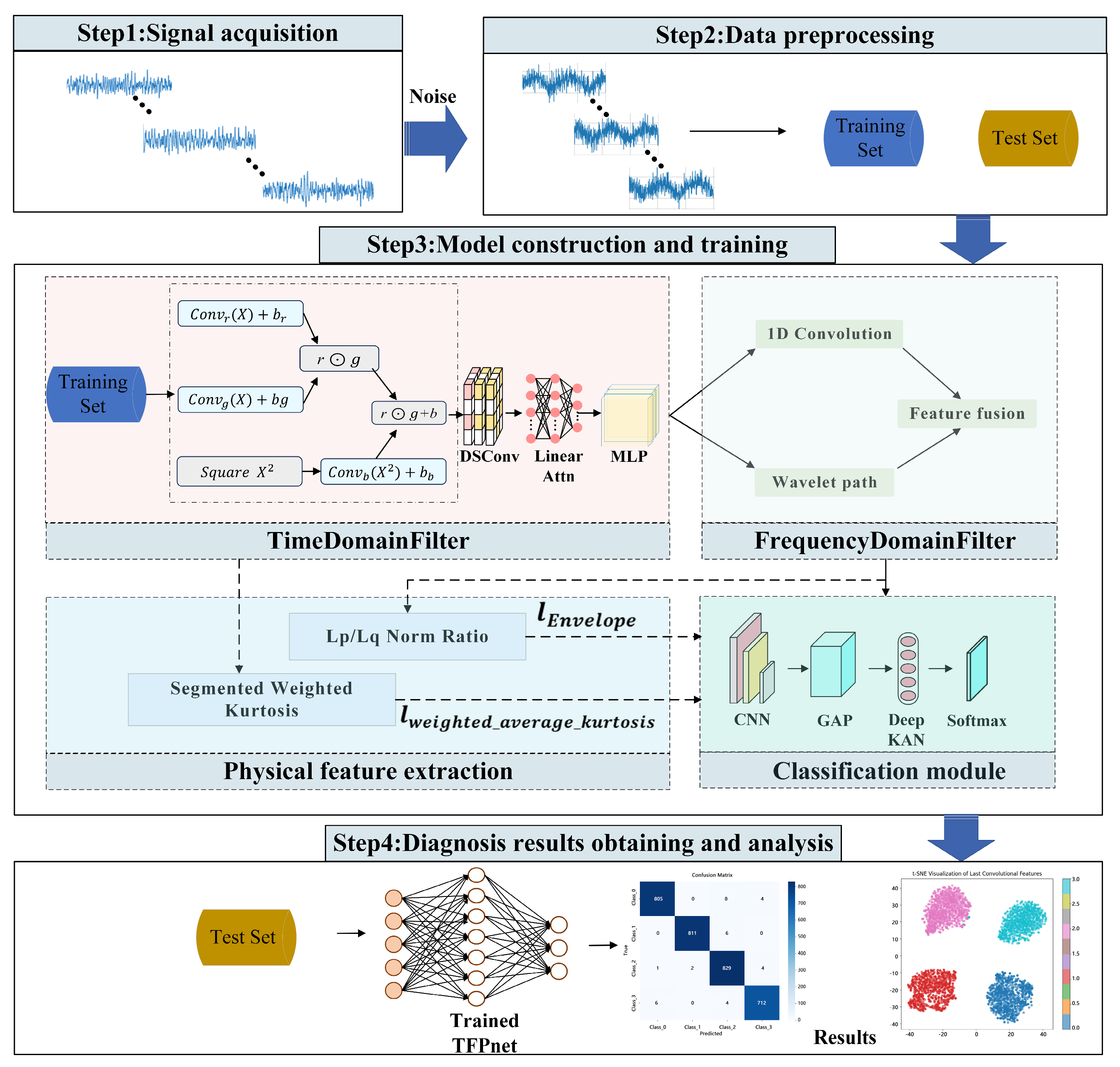
In this Section, we analyze the performance of the proposed TFPNet model through multiple sets of experimental results.

A.

Classification Results of TFPNet Model on Two Datasets

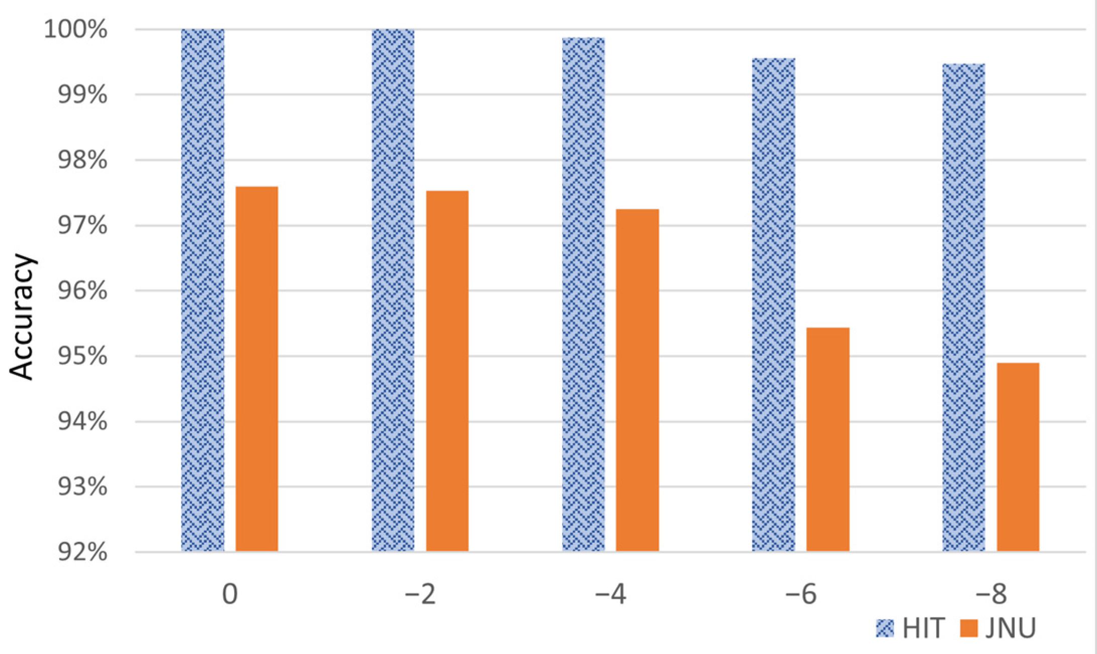
To evaluate the model’s stability under noise, we run the proposed model 10 times on both the training and testing sets, and report the average test accuracy as the final diagnostic performance. The accuracy of the proposed model on two datasets under different signal-to-noise ratios (SNR) is given in Figure 6. As the noise intensity increases, both datasets exhibit a gradual decline in classification accuracy.

The proposed TFPNet model maintains high fault detection performance even in strong noise backgrounds, demonstrating good robustness. Taking the HIT dataset as an example, the proposed model achieves perfect classification accuracy (100%) under an SNR of 0 dB, and even in a high-noise environment with an SNR of −8 dB, the model maintains a high accuracy of 98.78%. Similarly, on the JNU dataset, the model delivers robust performance, attaining 98.28% accuracy at 0 dB and still achieving 93.65% under the challenging −8 dB condition. These results demonstrate the model’s strong generalization capability across different scenarios, even in the presence of intense noise interference.

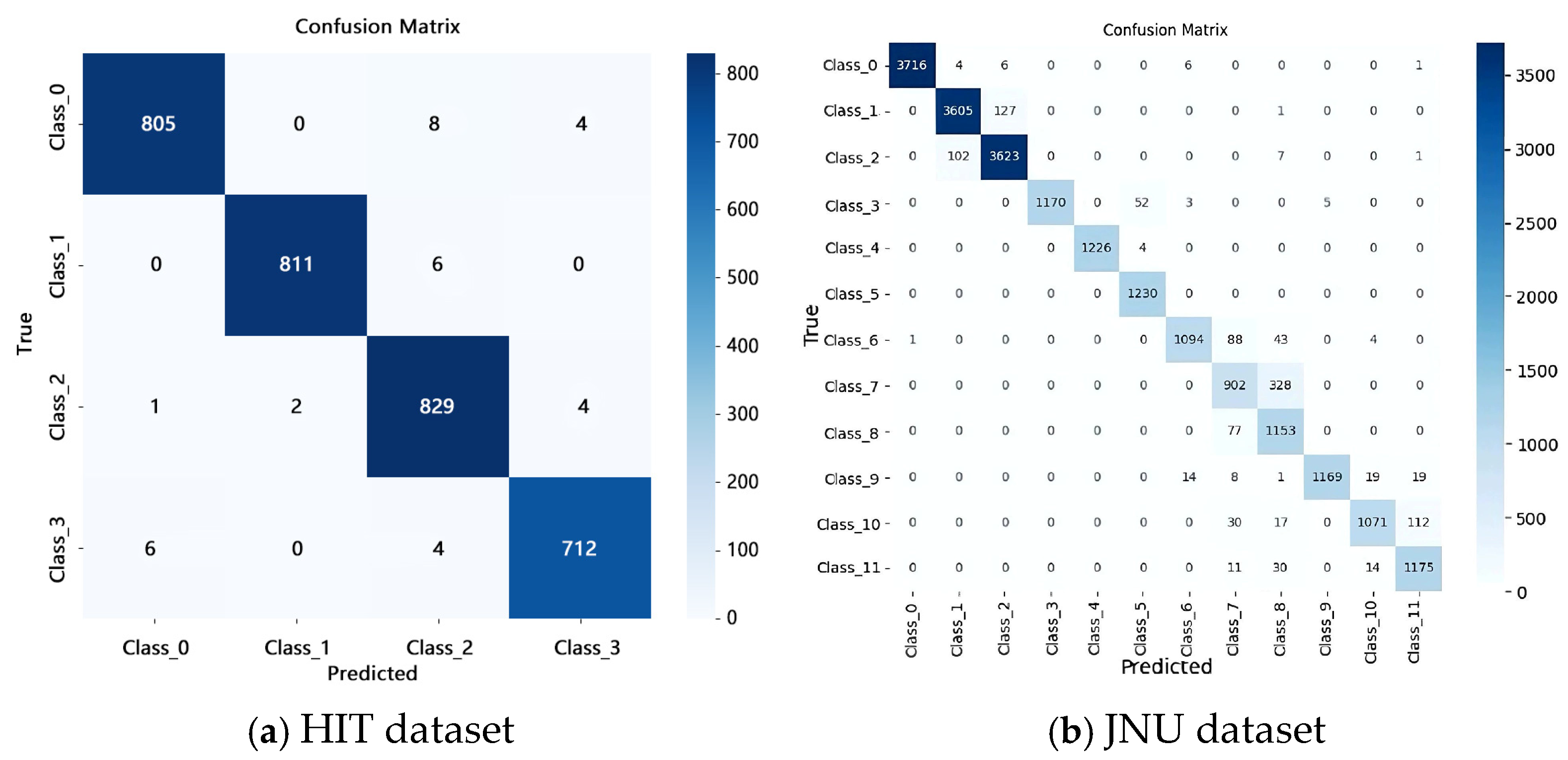
To further verify the discriminative ability of the proposed model in handling various types of bearing faults, confusion matrices are utilized to illustrate the correspondence between classification results and true labels. Diagnostic results on two datasets with a signal-to-noise ratio (SNR) of −8 dB demonstrate that TFPNet maintains high accuracy and fault distinction even under strong noise conditions. These results are given in Figure 7.

We conduct a qualitative analysis of data distribution using t-SNE under varying noise conditions (−8 dB, −4 dB, and 0 dB) to further demonstrate the model’s ability to classify and separate different sample categories in the feature space. The resulting two-dimensional embeddings are shown in Figure 8. Even at the lowest SNR of −8 dB, samples of the same class form compact clusters, while heterogeneous classes remain clearly separated, confirming the model’s robustness against strong noise.

B.

Ablation Experiment

In order to further evaluate the specific contributions of each module in the proposed TFPNet model, this Section conducts ablation experiments on accuracy. The following eight ablation models are specifically designed.

(1)

TFPNet-NoTime: This model completely removes the Time-Domain Filter and directly performs Fourier transform on the normalized signal, using the frequency spectrum as the input starting point to extract fault information from frequency domain features.

(2)

TFPNet-NoFreq: This model completely removes Frequency-Domain Filters and relies only on time domain features for subsequent classification, aiming to verify the impact of spectral filtering on fault detection performance.

(3)

TFPNet-NoAK: This model removes the weighted average kurtosis feature ak from the time-domain signal while retaining the spectral sparsity measure (Lp/Lq norm), verifying whether the model still has good representation ability without introducing time-domain statistical features.

(4)

TFPNet-NoG: This model removes the Lp/Lq spectral sparsity index g and retains the auxiliary branch based on weighted average kurtosis to explore whether the model still has good representation ability in the absence of spectral sparsity assistance.

(5)

TFPNet-NoAKG: This model simultaneously removes two auxiliary features, weighted average kurtosis ak and Lp/Lq norm g, and only retains the main classification path. It is used to test the basic performance of the model under the condition of complete dependence on the backbone structure, and verify the feasibility of the model without prior physical information assistance.

(6)

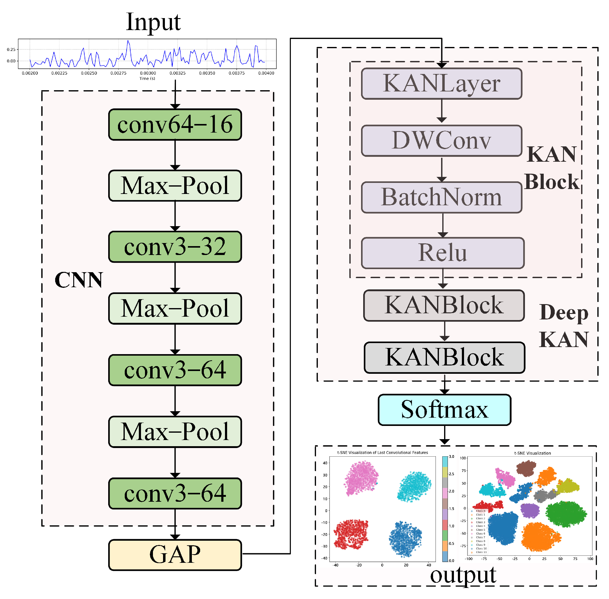
TFPNet-CNN: This model removes the DeepKAN module from the original structure and only retains the CNN backbone for feature extraction and classification, aiming to evaluate the improvement effect of the deep plasticity nonlinear modeling module (KAN) on the final performance.

(7)

TFPNet-Transformer: This model replaces the original classification feature extraction module with a Transformer architecture, explores the modeling ability of Transformer in fault detection tasks, and compares it with the original classification module.

(8)

TFPNet-ResNet: This model replaces the original classification feature extraction module with a ResNet like convolutional neural network structure, aiming to verify the effectiveness of the original classification model in modeling fault features.

The ablation experiment is conducted on the JNU dataset under the condition of SNR = −4 db. By comparing these ablation models, the effects of different modules on fault detection and diagnosis can be observed. The results are shown in

Table 2. Results of ablation experiment.

Model	Acc	F1	FPR
TFPNet	97.25%	96.47%	0.25%
TFPNet-NoTime	95.32%	93.93%	0.42%
TFPNet-NoFreq	91.11%	89.94%	0.82%
TFPNet-NoAK	95.77%	94.47%	0.38%
TFPNet-NoG	96.81%	95.85%	0.29%
TFPNet-NoAG	95.29%	93.69%	0.43%
TFPNet-CNN	86.20%	78.52%	1.23%
TFPNet-Transformer	80.60%	76.21%	1.78%
TFPNet-ResNet	92.15%	86.24%	0.70%

and Figure 9.

From the overall results in Table 2 and Figure 9, TFPNet performs the best in Acc (97.25%), F₁ score (96.47%), and FPR (0.25%), indicating that the collaborative fusion of each module plays a key role in performance improvement.

In the ablation experiment of Time–Frequency Domain Filters, TFPNet-NoTime and TFPNet-NoFreq remove the Time-Domain and Frequency-Domain Filters, respectively. The accuracy of TFPNet-NoFreq decreases to 91.11%, and the FPR increases to 0.82%, indicating that the spectral filter plays a more critical role in extracting weak fault information. The performance of TFPNet-NoTime is slightly better than TFPNet-NoFreq, but still lower than the original model, indicating the effectiveness of the Time-Domain Filter.

In the ablation experiment of the physical feature extraction module, the accuracy of TFPNet-NoAK and TFPNet-NoG are 95.77% and 96.81%, respectively, both slightly lower than the full model, indicating that the two have complementary enhancement effects on the model in different dimensions. Especially TFPNet-NoAKG shows a more significant performance decline after simultaneously removing ak and g (Acc of 95.29%, F₁ value decreased to 93.69%), further confirming the synergistic value of these two physical prior information.

In the ablation experiment of the classification feature extraction module, TFPNet-CNN only retains the convolutional feature extractor, and the accuracy significantly decreases to 86.20%, indicating that the feature mapping structure of KAN has stronger fault detection ability in the current task. After completely replacing the classification model with the Transformer architecture (TFPNet Transformer), the F₁ score further decreases to 80.60%, the F₁ value is only 76.21%, and the FPR increases to 1.78%, indicating that the Transformer’s modeling ability is unstable in low signal-to-noise ratio environments and it has difficultly handling complex signal feature extraction. In contrast, although TFPNet-ResNet outperforms the two mentioned above (with an accuracy of 92.15%), it is still significantly inferior to the original CNN-DeepKAN module, demonstrating the superiority of this classification module over mainstream convolutional neural networks.

In conclusion, the ablation experiment fully proves that the Time–Frequency Domain Filters, Physical Feature Extraction and Classification Model based on CNN and KAN in the TFPNet model play an important role in improving the diagnostic performance. The absence of any module will lead to performance degradation to varying degrees, which verifies the rationality and effectiveness of the overall architecture design.

C.

Comparative Experiment

In order to verify the performance of the TFPnet model proposed in this paper under noisy environments, it is compared with the three models, DRSN [29], Laplace Wavelet [30], and CSSTNet [31], under SNR-8-0db conditions, as shown in

Table 3. Comparison of results of four models on the two datasets (%).

Dataset	SNR/dB	TFPNet			DRSN			Laplace Wavelet			CSSTNet
		Acc	F1	FPR	Acc	F1	FPR	Acc	F1	FPR	Acc	F1	FPR
HIT	0	100	100.00	0.00	99.56	99.57	0.15	99.15	99.15	0.28	100	100.00	0.00
	−2	100	100.00	0.00	99.15	99.19	0.27	98.50	98.48	0.50	99.58	99.00	0.42
	−4	99.87	99.87	0.04	98.28	98.47	0.51	97.74	97.76	0.75	99.2	98.00	0.56
	−6	99.56	99.72	0.10	96.15	95.96	1.37	94.58	94.62	1.81	88.7	88.00	5.17
	−8	99.47	98.77	0.41	93.14	93.17	2.30	83.97	84.02	5.40	84.4	85.00	9.04
JNU	0	97.59	97.08	0.22	92.50	94.01	0.35	91.26	87.36	0.78	94.5	94.10	3.00
	−2	97.53	96.95	0.23	89.03	89.29	0.67	89.18	84.42	0.96	92.7	92.20	3.80
	−4	97.25	96.47	0.25	82.04	72.20	1.62	87.06	80.76	1.16	91.3	90.40	4.50
	−6	95.44	94.24	0.41	72.89	58.19	2.45	84.02	76.04	1.43	89.4	89.00	5.20
	−8	94.90	93.51	0.46	69.70	56.95	2.57	82.78	73.94	1.55	87.7	87.20	6.10

.

Table 3 shows that TFPNet consistently exhibits higher robustness and generalization ability under various noise environments. For the F₁ indicator, TFPNet achieves good performance under all SNR conditions, especially in the case of −6 dB and −8 dB strong noise, significantly higher than other models, demonstrating superior classification performance and stability.

Meanwhile, the average FPR of the proposed TFPNet is overall the lowest, far lower than the FPR levels of other models under the same conditions. This performance indicates that TFPNet can not only accurately identify real fault samples but also effectively suppress misjudgments under noise interference, improving availability and safety in industrial scenarios.

To more intuitively demonstrate the lightweight results of the proposed model, we compare the TFPNet model with the three models above, and results are given in

Table 4. Comparison Table of Parameters and Computational Amount of Benchmark Models.

Model	Params (M)	FLOPS (M)
TFPNet	0.0274	4.96
DRSN	0.03873	9.19
Laplace Wavelet	0.06443	5.83
CSSTNet	0.626008	69.72

. The total number of parameters and floating-point operations of the models are adopted to evaluate the complexity and computational cost of each model. Params (M) represents the total number of parameters of a model, in millions (Million). A smaller value usually indicates that the model is more compact and easier to deploy. FLOPs(M) represents the number of floating-point operations required for a model in a single forward inference process, also in millions (Million). A lower FLOPs value means the model has lower computational overhead and faster inference speed.

As shown in Table 4, TFPNet achieves the lowest parameter count (0.0274 M) and computational cost (4.96 M FLOPs) among all comparison models, representing only 4.4% and 7.1% of CSSTNet, respectively. Compared with other lightweight schemes, such as DRSN and Laplace Wavelet, TFPNet also demonstrates superior efficiency and compactness. These results indicate that the proposed model provides an obvious advantage for lightweight deployment while maintaining strong diagnostic performance.

At the same time, in order to demonstrate the performance of the proposed model, its results on the two datasets are compared with that of existing literature, as shown in

Table 5. Average accuracy with different SNR on the HIT dataset (%).

Model	SNR (Db)
	−6	−4	−2	0
MWRC [32]	96.33	97.72	98.69	98.95
TGAF-CNNT [33]	96.56	/	/	98.09
MD-BiMamba [34]	96.03	96.41	96.59	97.51
AWS-Ensemble [35]	/	95.28	97.78	99.17
TFPNet	99.56	99.87	100	100

and

Table 6. Average accuracy with different SNR on the JNU dataset (%).

Model	SNR (Db)
	−8	−6	−4	−2	0
WCNN-RSN [36]	/	85.27	88.39	90.83	93.77
KAN-HyperMP [37]	/	87.04	91.76	94.57	96.54
CSCohCNN [38]	83.89	86.24	89.34	91.59	92.48
MCRNet-GFK [38]	90.14	92.73	94.48	96.09	97.11
TFPNet	94.90	95.44	97.25	97.53	97.59

.

The above results indicate that the proposed TFPNet has demonstrated good accuracy in fault detection under different noise conditions, demonstrating that the design of the model framework can achieve bearing fault diagnosis under strong noise environments.

D.

Cross-Condition Experiment under a Noisy Environment

This Section evaluates the cross-domain diagnostic performance of the proposed model by designing six specific migration tasks under different speed switching.

The experiment used a sliding pane with a length of 2048 to sample healthy samples and various types of fault samples with a sampling rate of 50 kHz. The datasets at different operating speeds (600 RPM, 800 RPM, 1000 RPM) were represented by X, Y, and Z, respectively. The detailed migration instructions for the six migration tasks are shown in

Table 7. Task division for migration experiments.

Migration Tasks	Train RPM	Test RPM	Number of Training Samples	Number of Validation Samples	Number of Test Samples
Z→Y	1000 RPM	800 RPM	23,960	5990	29,950
Z→X	1000 RPM	600 RPM	23,960	5990	29,950
Y→X	800 RPM	600 RPM	23,960	5990	29,950
Y→Z	800 RPM	1000 RPM	23,960	5990	29,950
X→Y	600 RPM	800 RPM	23,960	5990	29,950
X→Z	600 RPM	1000 RPM	23,960	5990	29,950

.

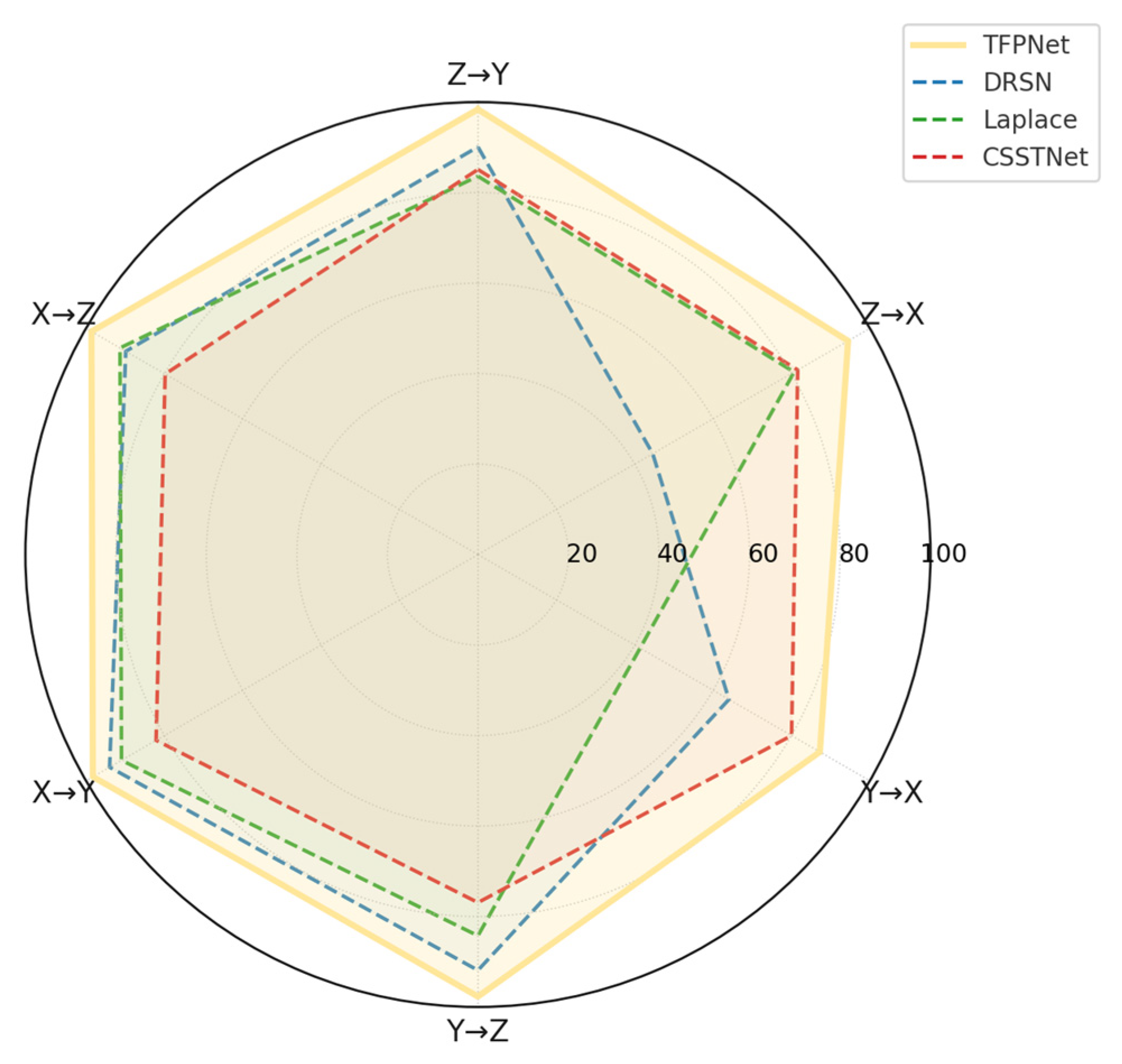
Six migration tasks are constructed to simulate domain shifts across different operating speeds for evaluating the transfer learning performance of the proposed model. As shown in

Table 8. Comparison results of migration task accuracy (%).

Model	Accuracy of Migration Tasks
	Z→Y	Z→X	Y→X	Y→Z	X→Y	X→Z	Average
TFPNet	98.41	94.44	87.24	97.70	98.25	98.62	95.78
DRSN	90.11	44.59	64.04	91.90	93.99	89.86	79.08
Laplace	83.63	80.67	41.38	84.26	90.95	91.33	78.70
CSSTNet	85.11	81.59	80.02	76.92	82.12	79.81	80.93

, TFPNet consistently achieves the best accuracy among all compared methods, with the highest reaching 98.62% (X→Z) and the lowest remaining above 87.24% (Y→X). In particular, for tasks with large speed disparities, such as Z→X and X→Z, the model still maintains high accuracy of 94.44% and 98.62%, respectively. The trend of classification performance across different transfer scenarios is further visualized in Figure 10, supporting the model’s robustness and adaptability to complex domain differences.

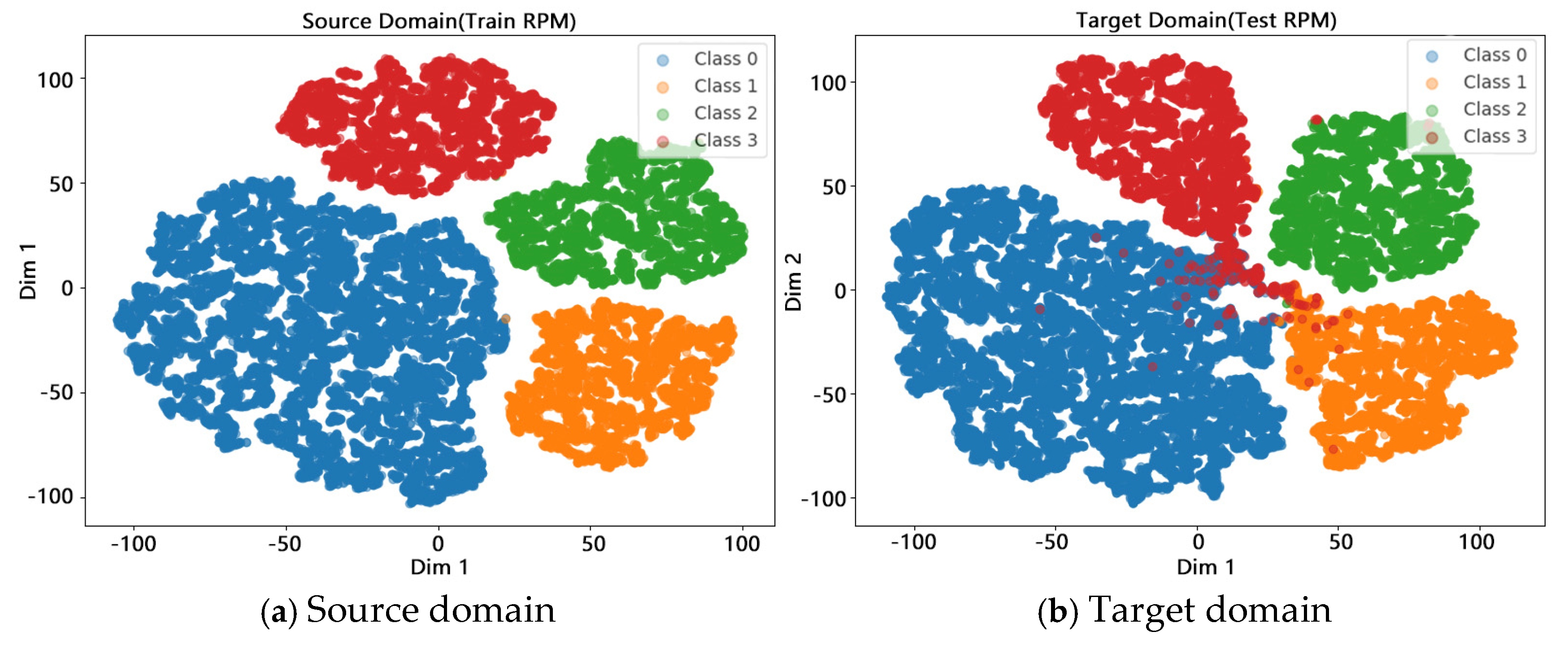
In order to observe the alignment effect of source domain (600 RPM) and target domain (1000 RPM) data with noise environment in the feature space more intuitively, this Section employs t-SNE algorithm for visual dimensionality reduction with SNR = −4 db, as shown in Figure 11. In Figure 11a, the distribution of the four classes of samples in the source domain shows a good clustering structure and is clearly separated from other categories.

Figure 11b shows that the clustering effect of various samples remains good after migration, with tight clustering of each cluster and stable feature distribution. There are a small number of boundary samples in Class 1 and Class 2 that shift towards the Class 0 region, resulting in some features being blurred. However, overall, the alignment effect of the source-target domain features in the latent space is good, which verifies the feature transfer and domain adaptation ability of the TFPNet model under different rotational speed conditions.

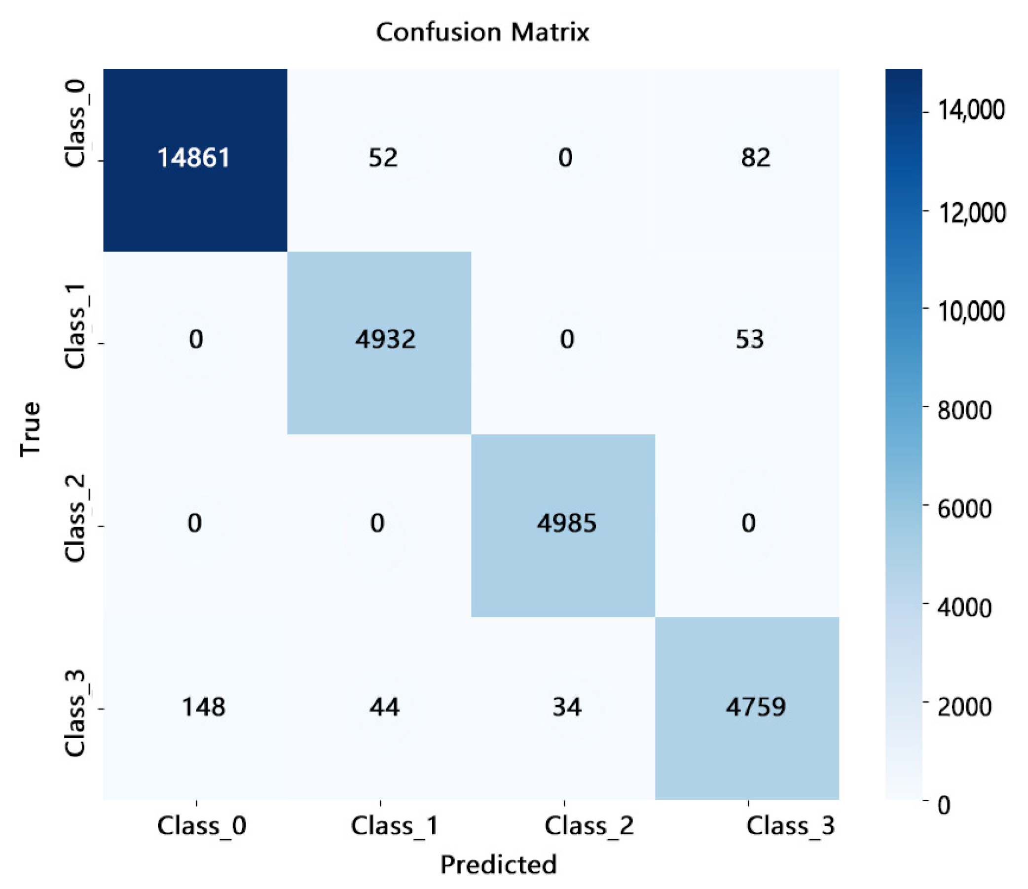
Confusion matrix is illustrated to further analyze the model performance on individual fault types in the target domain, as shown in Figure 12. Class 2 exhibits near-zero misclassification, indicating the model’s strong representational ability for this fault category. This observation is consistent with the clear separation of Class 2 in the t-SNE visualization. In contrast, misclassifications are observed between Class 0 and Class 3, particularly with approximately 2.8% of Class 3 samples being predicted as Class 0 or Class 1. This aligns with the partial overlap of these classes at the boundaries of the feature space in the t-SNE plot. Despite these local misclassifications, the overall diagnostic accuracy remains high, confirming the robustness and generalization capability of the proposed model in cross-condition fault diagnosis tasks.

5. Conclusions

Due to severe equipment wear and electromagnetic interference in ACTs, the equipment status data collected by sensors often contains noise, which affects the performance of equipment fault diagnosis. Therefore, a fault detection and diagnosis framework based on time–frequency domain filters and CNN-KAN is proposed for rolling bearings of equipment in ACTs under a noisy environment, which integrates four parts, including Time-Domain Filter, Frequency-Domain Filter, Physical Feature Extraction, and Classification Module. The proposed model is evaluated by multiple experiments on two public datasets, covering ablation experiments, comparison of results from multiple models, and comparison with the latest literature, and results show that the performance of the proposed model is better than other models, especially the stronger the noise, the better the accuracy, F₁, and FPR performance.

The large-scale equipment in ACTs needs to monitor numerous states, but the current number of state monitoring sensors deployed in the port is insufficient. Therefore, two publicly available datasets are employed for verification. In the future, if real-time production and environmental data can be obtained and utilized, it will greatly improve the accuracy and engineering applicability of fault detection and diagnosis models.