Abstract
Urban traffic signal coordination often prioritizes straight-through traffic, causing inefficiencies at intersections with high left-turn volumes. This study addresses left-turn traffic in path coordination control. First, using an enhanced FVD car-following model with acceleration decay and a minimum-jerk turning trajectory model, speed guidance is provided at intersections. For paths where left turns dominate, the traditional AM-BAND model is modified to maximize the green wave bandwidth for turning traffic and minimize carbon emissions, forming a multi-objective coordination control model with speed guidance. A case study was conducted on a typical path in Shanghai’s Jinqiao area. The results show that the left-turn-optimized model increases the green wave bandwidth by 16.67% over the traditional model, with an additional 9.52% improvement when speed guidance is included. For carbon emissions, the left-turn model reduces emissions by 12.99%, with a further 6.47% reduction under speed guidance. This approach effectively enhances efficiency and sustainability for left-turn-dominated paths, meeting urban commuter demands.
1. Introduction
In urban road networks, peak commuting hour traffic demand accounts for 10% to 12% of the total daily traffic volume (in most cities in China, such as Shanghai). Due to constraints such as urban industrial layout and road network distribution, a significant portion of commuting paths consist of multiple routes rather than a single arterial road. Particularly, left-turn traffic flows within these paths are prone to causing intersection congestion due to factors such as the turning radius and the length of intersections’ widening sections, significantly impacting the smoothness of urban traffic. On the other hand, vehicle speed guidance is a typical application of advanced driver assistance systems (ADASs). By providing real-time speed recommendations, this method enables vehicles to arrive at intersections during green phases, avoiding unnecessary stops. Therefore, considering how to implement speed guidance for left-turn traffic flows in commuting paths can “unblock” these flows, reducing travel time and alleviating network congestion.
Speed guidance is an effective method for improving the capacity of signalized intersections and reducing stop delays. Research on vehicle speed guidance by scholars both domestically and internationally has primarily focused on two aspects: intersection signal coordination and eco-driving. He et al. [1] proposed a multi-stage optimal control model aimed at optimizing vehicle trajectories on signal-controlled arterials by considering vehicle queues and traffic signal states. Peng Chen et al. [2] used a rolling optimization approach based on the spatiotemporal trajectories of vehicles to dynamically adjust the guidance speed for vehicles entering and exiting intersections, with the goal of minimizing energy consumption. However, this method only considered the speed of individual vehicles and lacked consideration of fleet speeds. Liu et al. [3] proposed a speed guidance algorithm in the context of the Internet of Vehicles, aiming to enhance traffic efficiency by optimizing the trajectories and timing of single or multiple vehicles. Ramin Niroumand et al. [4] employed a mixed-integer nonlinear equation to coordinate the control of autonomous and connected vehicles, integrating vehicle trajectories with traffic signal control to improve the efficiency of mixed traffic flows. Jing Binbin et al. [5] innovatively proposed a dual-cycle arterial green wave coordination control strategy, which focused on regulating vehicle acceleration and deceleration behaviors to optimize traffic flow. Xu Liping et al. [6] addressed issues in existing speed guidance models related to vehicle following and scenario division through real-time optimization in a vehicle–road cooperative environment, thereby improving intersection efficiency. Shi Qin et al. [7] adopted a fixed-duration speed guidance strategy targeting intelligent connected vehicle fleets, using Monte Carlo simulations to compare the effects of different guidance distances and durations on reducing fuel consumption and improving travel efficiency. Shi Qiuling et al. [8] optimized vehicle speed trajectories using Dijkstra’s algorithm and proposed a real-time variable speed guidance strategy to reduce energy consumption and improve traffic efficiency under varying traffic volumes.
The existing research on signal coordination control mainly focuses on the integration of speed guidance and signal timing optimization. Biao et al. [9] developed a cooperative optimization strategy that combines signal timing with speed optimization, aiming to simultaneously improve signal timing efficiency and vehicle travel speed. This strategy includes roadside traffic signal optimization and onboard speed control components. Zhang Jingsi et al. [10] constructed a multi-objective optimization model for dual-cycle arterials under speed guidance, with optimization goals including arterial delay, capacity, stop frequency, and minor road delay at dual-cycle intersections. They also proposed a dynamic speed guidance model considering queue dissipation and phase difference for different traffic flow conditions at upstream intersections. Wang Xu [11] aimed to minimize arterial fleet delay while also considering the minimization of fleet emissions as a secondary objective. They built an optimization model for arterial signal coordination control that accounts for fleet emissions and proposed a solution method combining the tolerant hierarchical sequence method with the branch-and-bound method. Deng Mingjun [12], in a vehicle–road cooperative environment, used the Maxband model to construct a multi-objective optimization model for arterial signal coordination, aiming to maximize the green wave bandwidth and minimize arterial vehicle delay, stop frequency, and minor road delay. This study not only obtained global control scheme parameters for coordinated intersections, but also proposed a speed guidance model based on the position of vehicles at intersection approaches and signal states, significantly enhancing the efficiency of arterial coordination control.
Current research on urban path speed guidance predominantly focuses on guiding straight-through traffic flows in the main direction. For left-turn traffic flows, considerations mainly include the impact of left-turn merging and the sequence of phase releases. For example, Xu Jianmin et al. [13] proposed two phase release strategies for left-turn traffic flows at T-intersections and established a green wave coordination control model aimed at maximizing the bidirectional green wave bandwidth. Yang Xiaofang et al. [14] considered the influence of merging left-turn vehicles by determining the passable time for both straight-through and merging left-turn vehicles on arterials, guiding left-turn and straight-through flows to maximize efficiency through arterial coordination control. However, this approach lacks consideration of the merging time of left-turn flows and the issue of vehicle queuing.
In summary, the existing research primarily focuses on speed guidance for straight-through traffic flows, with limited attention paid to left-turn flows, particularly the car-following behavior in speed guidance for left-turning vehicles. Therefore, this study integrates the minimum-jerk theory to plan the internal left-turn trajectories of left-turn traffic flows at intersections, calculates the left-turn time, and considers the impact of acceleration and deceleration attenuation on following vehicles. By providing optimal guidance speeds for following vehicles, a speed guidance model for left-turn vehicles is established, enhancing the accuracy of speed guidance for left-turn flows. Building on this, for paths where left-turn flows dominate between upstream and downstream intersections, a multi-objective coordinated control model considering speed guidance is constructed based on the AM-BAND variable bandwidth model. The optimization objectives include maximizing the green wave bandwidth for turning flows and minimizing paths’ carbon emissions, thereby improving the coordination control capability of paths with left-turn flows.
2. Speed Guidance for Path Traffic Flows
2.1. Basic Assumptions and Research Scope
To simplify the research problem, the proposed model in this study is based on the following basic assumptions:
- All vehicles’ onboard devices can connect with roadside devices and receive real-time data, with negligible communication latency;
- Guided vehicles strictly follow the speed guidance strategy;
- Vehicles do not change lanes after entering the guidance zone.
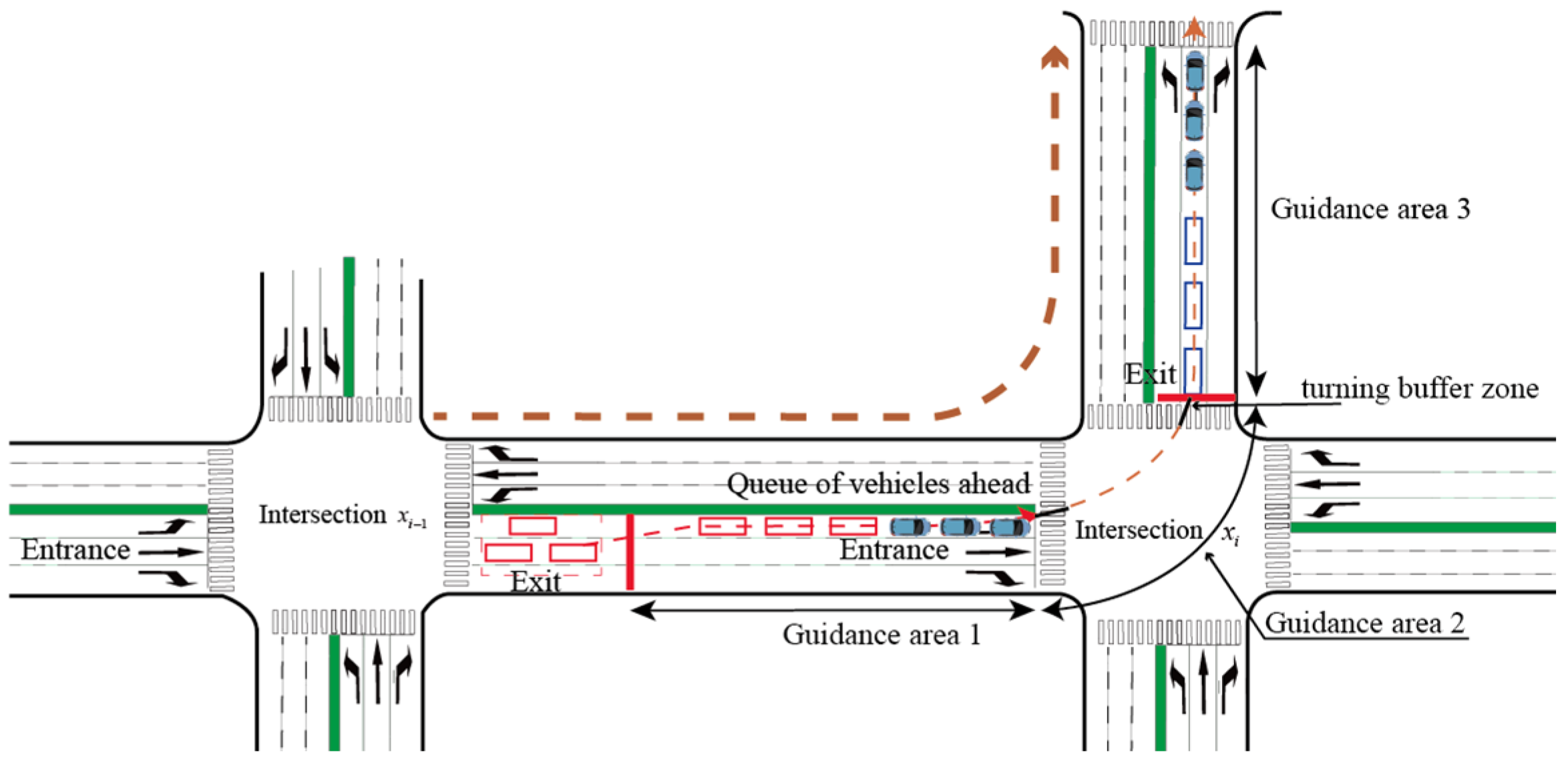
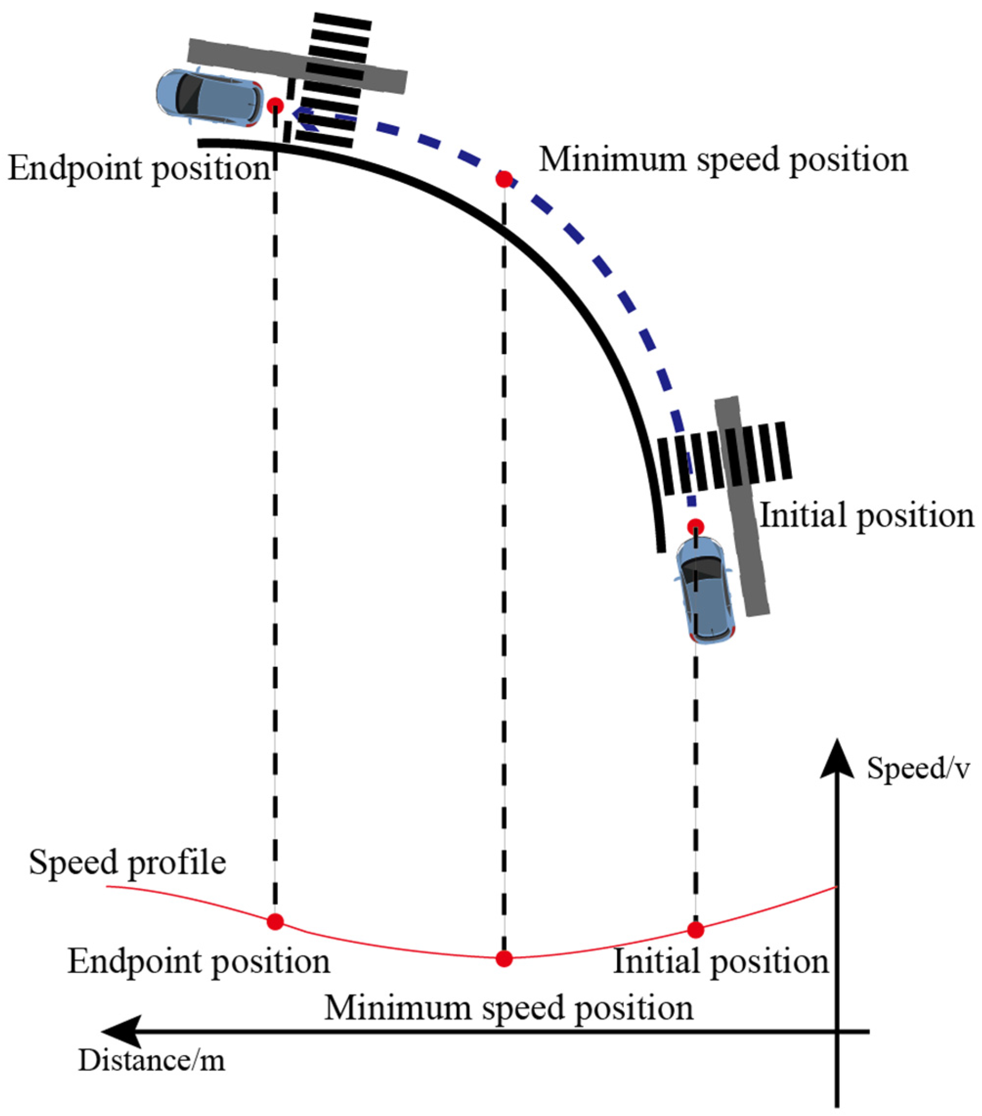
In this study, two adjacent intersections are selected as the research subjects (Figure 1). These two intersections form part of a path, with a focus on the left-turn behavior at these intersections (go straight at the intersection , then turn left at the intersection , and proceed in the direction indicated by the orange dashed arrow in Figure 1), particularly the process from the completion of merging at the intersection to the end of the left-turn queue at the intersection . Vehicles merge at the exit lane of the intersection and, when approaching the entrance lane of the intersection , typically form orderly queues. Therefore, a speed guidance area is established at a certain distance before the entrance lane to ensure that vehicles form a queue and are guided to pass through the left-turn intersection (intersection ) without stopping, proceeding to the next intersection.
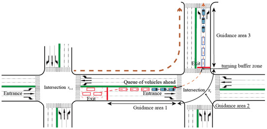
Figure 1.
Speed guidance areas diagram.
The entire path speed guidance model is divided into two stages. The first stage is straight-through speed guidance, where speed guidance is applied on the straight section before the intersection turn. The second stage is turn-phase speed guidance, which includes determining the left-turn guidance speed within the intersection and the straight-through speed guidance after leaving the left-turn intersection and before reaching the next intersection.
2.2. Vehicle Acceleration Decay Car-Following Model
2.2.1. Acceleration Decay Model
This paper focuses on speed guidance for left-turning vehicle platoons. Upon entering the guidance zone, different guidance methods are employed. The acceleration or deceleration of the lead vehicle inevitably influences the speeds of the following vehicles, leading to changes in driving characteristics. Therefore, it is necessary to improve the traditional car-following model under conventional conditions. Drawing on the path loss propagation model, an FVD (Full Velocity Difference) model considering acceleration attenuation is established:
where denotes the attenuation value of the acceleration signal from the leading vehicle to the following vehicle at time , when the distance between the leading and following vehicles is . When the leading vehicle is accelerating, , otherwise, ; denotes the minimum following distance. denotes the acceleration loss exponent factor, which is primarily related to the headway spacing, vehicle type, and spatial traffic environment. This paper mainly selects headway spacing as the characterizing factor. As varies, may take different values to characterize the attenuation of the acceleration signal under different following distances. denotes the random error term.
By substituting into the equation and ignoring the random error term, a simplified attenuation model can be obtained:
2.2.2. FVD Car-Following Model with Left-Turn Acceleration Decay
Based on the acceleration decay model, the Full Velocity Difference (FVD) car-following model is improved to form a vehicle queue with the following vehicles and the leading vehicle guided by the same target speed, allowing the platoon to pass the intersection stop line with minimal or no stopping during the green light. The improved FVD car-following model, which considers acceleration decay and the safe distance between vehicles, is expressed as follows:
where is the updated following acceleration of the n-th vehicle, ; is the driver sensitivity coefficient, with a value of 0.41 ; is the feedback coefficient, with a value of 0.3 ; is the speed optimization function considering safe spacing; is the speed difference between the leading and following vehicles; denotes the safe vehicle spacing; denotes the maximum driving speed; denotes the driver’s reaction time, taken as ; and Lis the length of the leading vehicle.
The impact of acceleration decay on the stability of the FVD car-following model mainly refers to Li Jiachen [15]. Furthermore, in Kesting A [16]’s research, when performing trajectory fitting for different car-following models, it was found that introducing delays had almost no impact on the fitting error. This indicates that even with different model structures, the influence on the macroscopic traffic flow behavior is limited, thereby suggesting that the impact on coordination control differences in the coordinated control system can be considered limited. Therefore, this paper does not compare the modified FVD model with other models, nor does it conduct stability tests on it. In the traditional FVD model, the influence of the turning radius on the sensitivity coefficient and parameters during the actual car-following process of vehicles turning at intersections is not considered. Additionally, during the left-turn car-following process, the turning speed must be optimized and adjusted due to the influence of the turning radius. Vehicles need to decelerate in advance before reaching the intersection to turn at a reasonable speed and then follow the leading vehicle in the corresponding lane. After passing through the intersection, to prevent excessive acceleration, the optimized speed of the turning vehicle should not change abruptly, but should gradually increase while ensuring driving safety and passenger comfort. To ensure that the vehicle does not collide with the leading vehicle and that the turning speed is as close as possible to the optimized speed, considerations of the turning radius and safe spacing are incorporated into the traditional FVD model, resulting in the optimized left-turn FVD model (9):
In the equation, and denote sensitivity coefficients considering the turning radius, with values that vary according to the turning radius; denotes the optimized speed function considering the left-turn radius; denotes the speed optimization coefficient function at different turning positions; denotes the buffer distance for the deceleration of turning vehicles; denotes the position of the stop line; denotes the position of the n-th following vehicle; and denotes the turning coefficient of the vehicle, where a larger indicates a higher turning speed of the vehicle.
For the sensitivity coefficients related to the turning radius, this paper refers to the parameters calibrated by Wei Fulu et al. [17] through iterative calculations using a genetic algorithm, obtaining the final values of the parameters in the model for different turning radii at signalized intersections, shown in Table 1 and Table 2.

Table 1.
Sensitivity coefficients for left turns in the modified FVD car-following model.
Table 2.
Improved FVD car-following model sensitivity and feedback coefficients.
The assumption conditions for parameters k and λ are the asymmetric response assumption and the safety distance correlation assumption: the following vehicle’s driver’s response to the acceleration and deceleration behaviors of the leading vehicle is asymmetric, that is, the sensitivity during deceleration is higher than that during acceleration. Therefore, the model divides the parameters into acceleration sensitivity coefficients and deceleration sensitivity coefficients. This paper mainly adopts the assumption of its deceleration sensitivity coefficients. In addition, the parameter values are related to the safety vehicle distance model, which comprehensively considers factors such as vehicle speed, acceleration, driver reaction time, and vehicle length.
The application scope of parameters k and λ is applicable to the turning and through behaviors of vehicles at urban signalized intersections under sunny conditions, and the vehicle speed during turning should be between 24.5 km/h and 19.5 km/h.
During the guidance process, there is a straight-through car-following process from the speed guidance point to before the stop line and a turning process when entering the intersection. Therefore, the FVD model considering acceleration decay is as follows (Equation (10)):
2.3. Speed Guidance for Left-Turn Commuter Paths
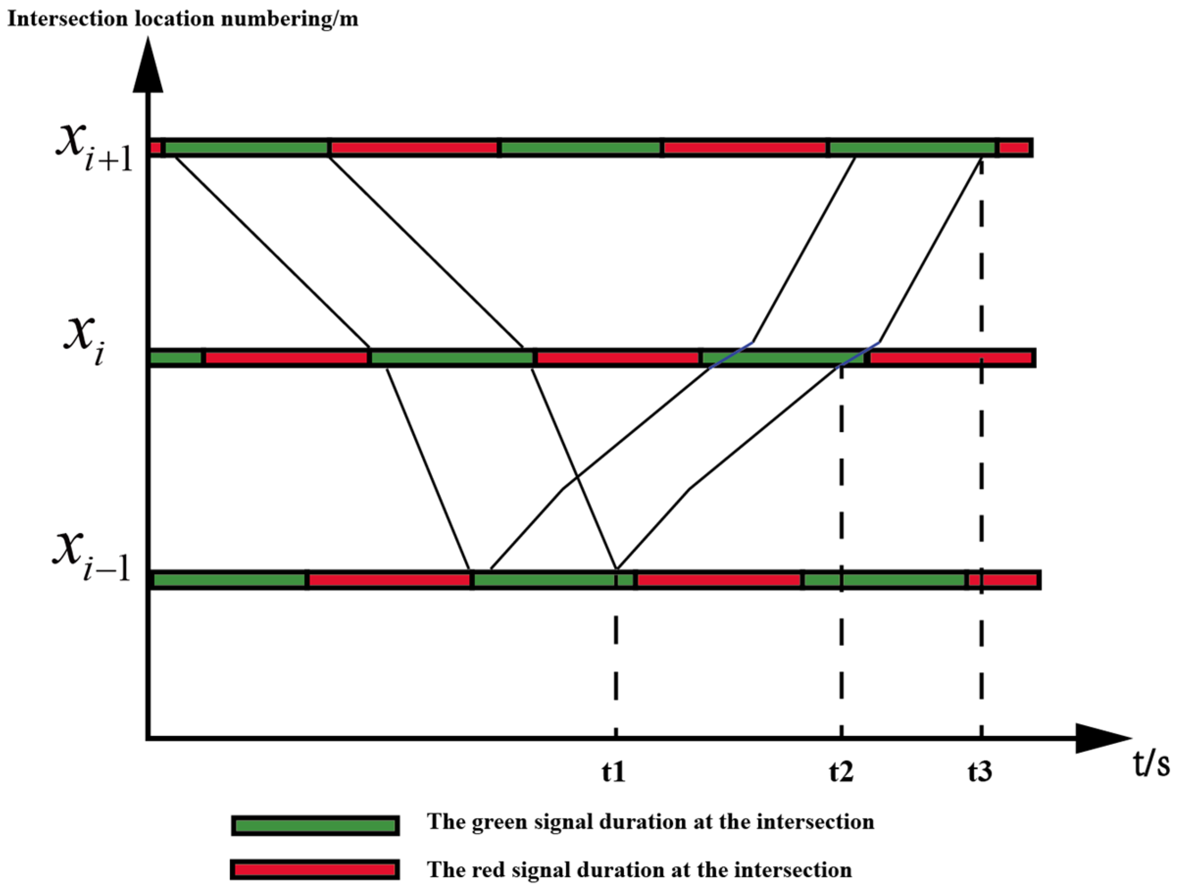
According to the time–distance diagram in Figure 2, the horizontal axis represents the time axis, the vertical axis represents the intersection location, the diagonal line represents the vehicle’s trajectory, while its slope indicates the vehicle speed. Here, t2–t1 denotes the travel time between intersection and intersection ; t3 − t2 denotes the travel time between intersection and intersection ; and the red–green bars in the middle represent the traffic light status at the intersection. Taking the upstream direction as an example, is a left-turn intersection and intersections and are the upstream and downstream straight-through intersections of the left-turn intersection, respectively. The traffic flow passing through the intersection during the green light is divided into two categories: straight-through speed traffic flow at intersections and , and left-turn speed traffic flow at intersection . Clearly, the guidance speed is affected by the intersection phase difference and left-turn turning radius. Therefore, analyzing the relationship between the speed, phase difference, and left-turn turning radius is necessary for establishing the speed guidance model. The speed guidance is divided into two stages: straight-through speed guidance and left-turn speed guidance.

Figure 2.
Time–distance diagram.
The straight-through stage guidance mainly determines the guidance speed for the straight-through lead vehicle based on the vehicle’s arrival time and phase difference. The following vehicles’ following acceleration is determined based on the lead vehicle’s speed using the acceleration decay car-following model. In the left-turn stage, the lead vehicle’s speed is determined by the left-turn lead vehicle’s guidance speed based on the minimum-jerk trajectory planning. Subsequently, the straight-through guidance speed after the left turn is determined based on the phase difference. The following vehicles’ acceleration in the left-turn stage is determined by the car-following model under left-turn speed optimization.
2.3.1. Speed Guidance in the Straight-Through Phase
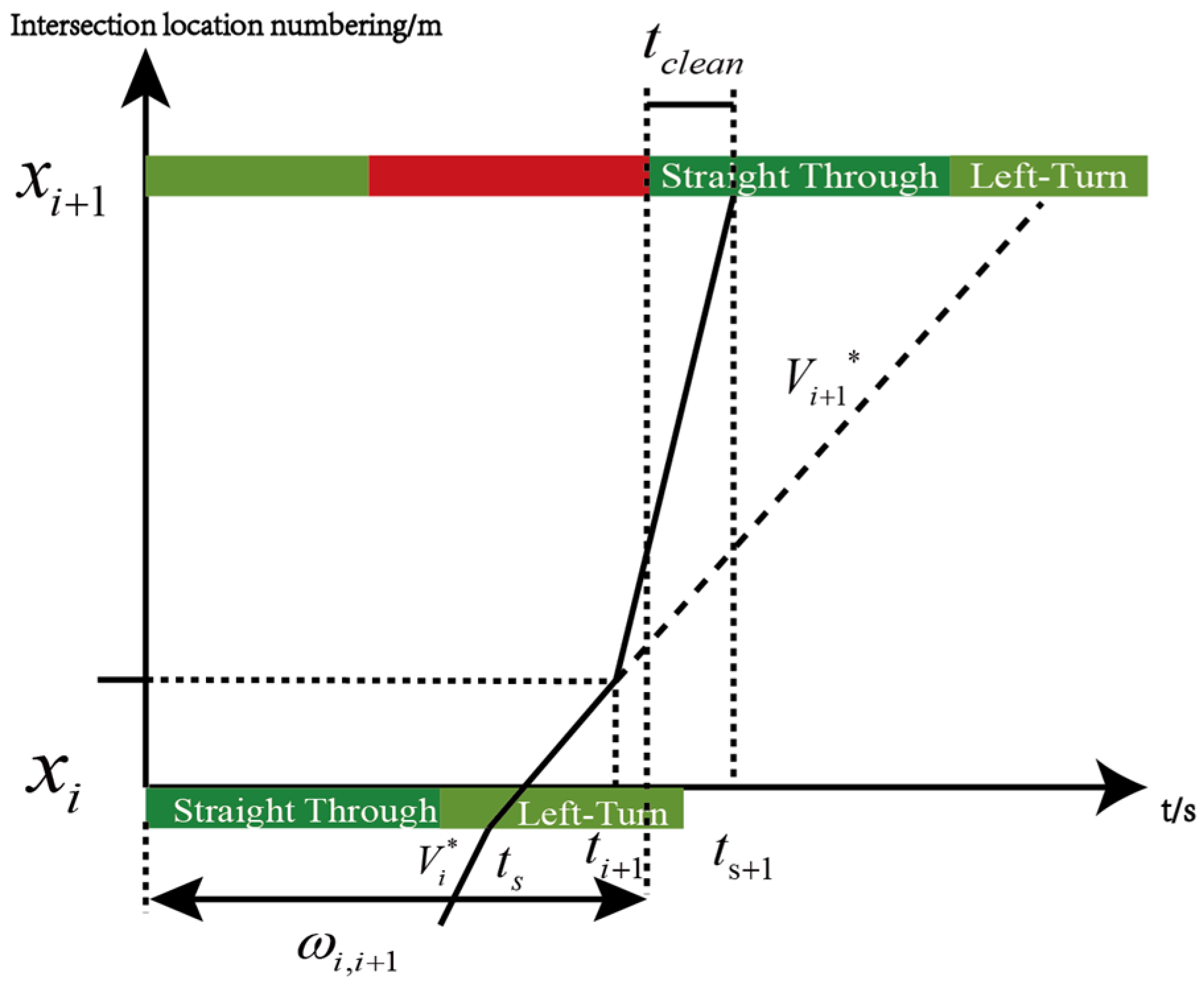
The speed guidance in the straight-through phase is shown in Figure 3 (the diagonal line drawn with a dashed line represents the time to reach the next intersection at the original speed, while the diagonal line drawn with a solid line represents the time to reach the intersection at the guided speed). The guided vehicle exits from intersection , and since a left turn is required at intersection , if the vehicle travels at the initial speed, it will arrive during the straight-through green light. Therefore, after entering the guidance area, deceleration guidance is needed, and the guidance speed at this time is .
where denotes the length of the guidance zone; denotes the phase difference between intersections and in the coordination direction; denotes the straight-through green time; denotes the queue clearance time; and denotes the time for the vehicle to reach the speed guidance zone.
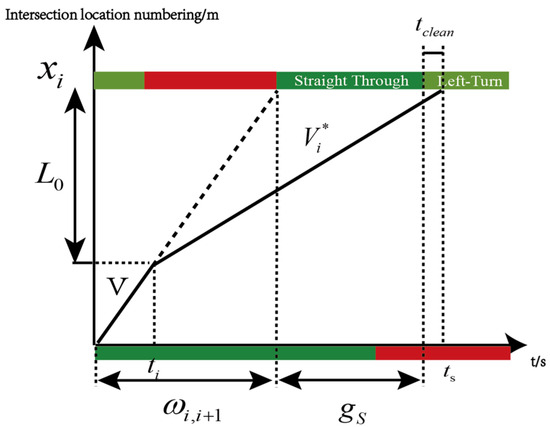
Figure 3.
Speed guidance in the through phase.
The following vehicle’s acceleration is given using the following:
where denotes the driver sensitivity coefficient, with a value of 0.41 ; denotes the feedback coefficient, with a value of 0.3 .
2.3.2. Speed Guidance in the Left-Turn Phase
- Speed guidance at left-turn intersections
The left-turn trajectory planning model studied in this paper is based on the minimum-jerk principle [18]. This method is primarily used to describe the inertial motion of objects in a two-dimensional plane. Flash and Hogan demonstrated that the smoothness of inertial movements (such as reaching, writing, and drawing tasks) can be represented by an acceleration function. To ensure smooth turning, the trajectory is formulated by minimizing the objective cost function within a specified time , the sum of the squared accelerations along the movement direction from a given initial position to the target position. The function is expressed as follows:
where denotes the vector sum of the smooth movement of the end effector from one position to another; denotes the motion time from the starting position to the target position; denotes the x-coordinate of the object’s position at time ; and denotes the y-coordinate of the object’s position at time .
For convenience in calculation, the solution to the objective cost function is represented by two fifth-order polynomials of time:
where and () denote the constant coefficients.
Equations (14) and (15) contain 12 constant coefficients, which indicates that there are 12 unknowns. Therefore, solving these equations requires 12 boundary conditions. The vehicle’s initial and target positions (the coordinates of and ), velocity vectors, and acceleration vectors (the components of and ) can provide these 12 boundary conditions. The coordinates of the initial and target positions of the vehicle’s trajectory can be obtained from the intersection location and its surrounding geometric data. The vehicle’s velocity and acceleration at the entry and exit points depend on the speed characteristics when entering and exiting.
Vehicles on commuting routes often appear in the form of a convoy, and determining the guide speed of the lead vehicle is crucial for determining the convoy’s speed. This paper applies the minimum-jerk theory to plan the trajectory of the lead vehicle in the left-turn traffic flow, thereby determining the guide speed of the lead vehicle.
Traditional trajectory models use the starting and target positions, velocities, accelerations, and the motion time () between these positions as trajectory information, and it is explained that the trajectory of turning vehicles under free-flow conditions can be described using the minimum-jerk principle. Although the applicability of the minimum-jerk principle to turning vehicles has been proven [19], it does not take into account the influence of intersection geometry. Furthermore, this model requires the input of which is information that cannot be obtained. Therefore, this paper does not choose to use the motion time from the starting position to the target position, but instead uses the position and velocity information of intermediate points to estimate the left-turn trajectory. By combining Equations (14) and (15), the unknowns can be estimated, providing the left-turn movement time within the intersection for the speed guidance model, thereby improving the accuracy of speed guidance for the left-turn traffic flow.
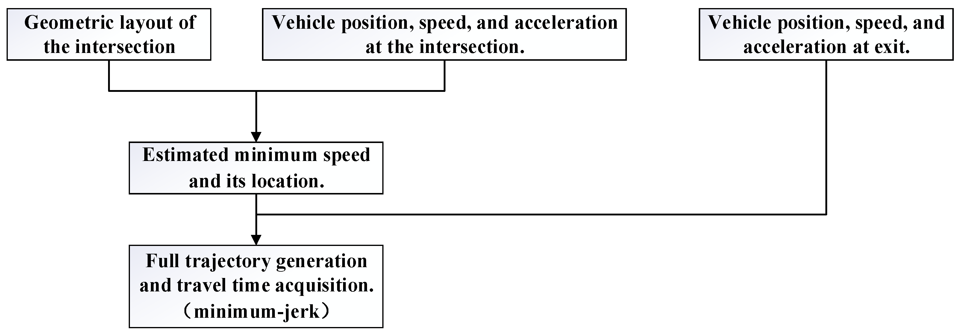
The position information on intermediate points in the left-turn trajectory (minimum speed and the location of minimum speed) is estimated using the model proposed by Wolfermann et al. The specific structure of the left-turn trajectory planning model is shown in Figure 4. The input variables include the vehicle type and the geometric state of the intersection (intersection turning angle, curb radius, and lateral exit distance, with each parameter defined as shown in Figure 5). The conditions for the lead vehicle when entering and exiting the intersection (position, speed, and acceleration) are also considered. The minimum speed and the location of the minimum speed are then selected from the probability model of the normal distribution estimated by Wolfermann.
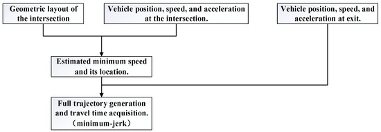
Figure 4.
Left-turn trajectory planning model.
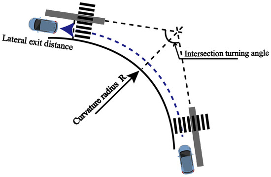
Figure 5.
Definition of parameters in the intersection model.
By combining the minimum-jerk theory with the velocity prediction model proposed by Wolfermann, the corresponding synchronization equations can be obtained. The specific relationship between position and velocity is shown in Figure 6. It can be seen that the speed of the lead vehicle in a left turn decreases from the initial position until it reaches the minimum speed, and then gradually increases to reach the corresponding target speed. Therefore, selecting three points—the initial position, the minimum speed position, and the target position—for predicting the turning trajectory will better align with the actual situation:
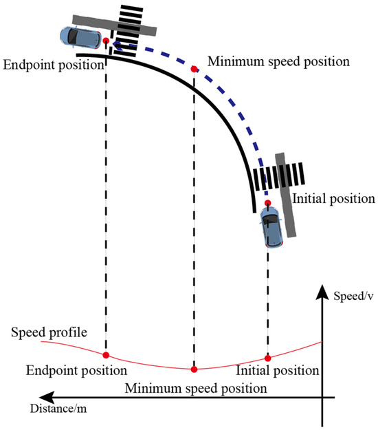
Figure 6.
Position and velocity correspondence of the left-turn lead vehicle’s driving path.
The initial position of the trajectory is defined as follows:
where , and denote the starting point position, velocity, and acceleration of the turning vehicle, respectively, all of which are known. For convenience in calculation, the starting point position is set as (0, 0).
According to the minimum-jerk theory, the target position of the trajectory can be defined as follows:
where , , and denote the position, velocity, and acceleration of the left-turn lead vehicle at the known target position, respectively.
Similarly, the minimum speed and the position of the minimum speed can be defined as follows:
where , and denote the position, velocity, and acceleration of the left-turn lead vehicle at the minimum speed. These values can be estimated using Wolfermann’s model, where and follow a Gaussian distribution. Based on the distribution values, and can be randomly selected and substituted into Equation (18) for calculation.
Wolfermann’s model estimates the minimum speed and the position of the minimum speed for turning vehicles under ideal or free-flow conditions based on the historical data of left-turn vehicles. It then transforms these estimates into a functional model that takes into account the entry speed and the geometric characteristics of the intersection. Table 3 lists the parameters of the minimum speed () and the position of the minimum speed () models. The representations of and are modeled using normal distributions, with the mean () and standard deviation () modeled as functions of the entry speed and intersection geometric characteristics. The definitions of the model parameters are shown in Figure 5.
Table 3.
Normal distribution model for minimum speed and minimum speed position of turning vehicles.
Since and are still unknown, but the vehicle is at the minimum speed at this point, we can assume . By solving the system of equations formed by Equations (16)–(18), we can obtain the turning movement time for the turning vehicle.
The turning vehicle trajectory derived from the minimum-jerk theory takes into account the left-turn safe speed. Based on this, the guide speed of the vehicle within the intersection is obtained. The calculation model for the lead vehicle’s guide speed is as follows:
Under weather conditions such as rainy days, snowy days, and freezing days, the road surface will become wet and slippery due to moisture, water accumulation, snow accumulation, ice, or covering with pollutants, resulting in abrupt changes in the road surface friction coefficient, which will have adverse effects on road traffic and driving safety. Therefore, this study introduces the road surface wet and slippery friction coefficient in the determination of the left-turn safe speed, and obtains the safe guiding speed for the head vehicle to turn left.
Among them, the wet and slippery friction coefficient of the road surface is determined according to the friction coefficient range of different road surface conditions proposed by Li Changcheng et al. [20]. The specific values of the wet and slippery friction coefficient of the road surface are shown in the Table 4.
Table 4.
The range of wet–slippery friction coefficients for different road surface conditions.
At this point, the acceleration of the following vehicle can be calculated using the following method:
where is the driver sensitivity coefficient; is the feedback coefficient. Determine based on Table 2.
- 2.
- Straight-through stage speed guidance after left-turn completion
The vehicle needs to make a left turn and then continue straight through the intersection . If the vehicle travels at the left-turn guide speed , it will not be able to arrive at the next intersection when the green light turns on. Therefore, the vehicle needs to travel at a speed until the next green light phase starts, shown in Figure 7. The guide formula for this is as follows:
where denotes the time to enter the intersection guide zone; denotes the phase difference between the coordinated directions of intersection and intersection.
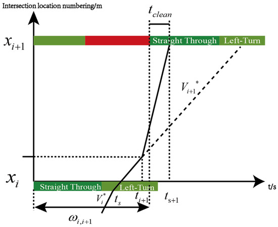
Figure 7.
Left-turn stage speed guidance.
At this point, the acceleration of the following vehicle can be calculated using Equation (22):
where is the driver sensitivity coefficient, with a value of 0.41 ; is the feedback coefficient, with a value of 0.3 .
2.3.3. Speed Transition Between Through and Left-Turn Phases
To ensure that the speed and acceleration transitions between the through phase and left-turn phase comply with physical authenticity and numerical stability, this paper introduces a weighted interpolation smoothing function to construct a continuously differentiable transition model. This model prevents abrupt changes in vehicle speed, thereby improving the simulation accuracy and control effect of the model.
Suppose the vehicle leaves the through phase at time and enters the left-turn phase at time , with the intermediate transition time being .
In the transition interval, the vehicle speed can be expressed as follows:
- The transition speed from the through phase to the left-turn phase:
- 2.
- The transition speed from the left-turn phase to the through phase:
3. Multi-Objective Optimization for Left-Turn Path Coordination Control Under Speed Guidance
To achieve the optimal state of the guidance model, this paper uses the AM-BAND green wave bandwidth model and the carbon emission model as optimization objectives for multi-objective optimization. The goal is to maximize the green wave bandwidth in the direction of path coordination control while minimizing carbon emissions. This ensures that, under the maximum traffic capacity, vehicle travel is greener and has lower carbon emissions, reducing energy consumption.
3.1. Green Wave Bandwidth Model
The AM-BAND model [21] removes the symmetrical constraint of the green wave bandwidth while adding a constraint on the left–right bandwidth ratio, allowing for different bandwidths between intersections. Its objective function is as follows:
where B denotes the weighted sum of the bandwidths for both the up and down directions, and i is the intersection number. is the weight value of the green wave bandwidth for the up (or down) direction on the road segment between intersections , denotes the actual traffic volume in the up (or down) direction on the road segment, and denotes the saturated traffic volume in the up (or down) direction on the road segment. The exponent p can take values of 0, 1, or 2. denotes the green wave bandwidth from intersection to , in which , .
Due to the imbalance in the traffic volume between upstream and downstream on the commuting path, the parameter is set to ensure balance.
where denotes the bandwidth demand ratio between the downlink and uplink directions, which is typically the ratio of the traffic flow in the downlink direction to the traffic flow in the uplink direction.
To determine the upper and lower bounds for each intersection cycle:
where and are the upper and lower limits of the signal cycle, respectively.
By setting interference constraints, the green wave bandwidth in the up and down directions is ensured not to overlap with the red light signal timing, thereby reducing the stoppages and delays caused by red light signals:
where denotes the time difference between the centerline of the green wave bandwidth in the coordinated direction (up or down) at intersection and the edge of the adjacent red light on the left (or right) side. is the queue clearance time in the coordinated direction (up or down) at intersection . denotes the red light time in the coordinated direction (up or down) at intersection .
To prevent the progression band component from becoming too large or too small and thereby maintain the balance of the progression band:
The cycle constraint:
where denotes the travel time for a vehicle from intersection to intersection ; denotes the 0–1 variable used to determine the coordination direction’s straight-through and left-turn-phase sequence. is the duration of the left-turn green light in the up (or down) direction at intersection ; denotes the multiple of cycle, .
The speed constraint:
in which denotes the distance from intersection to intersection in the up (or down) direction. denotes the minimum and maximum vehicle speeds, respectively, on the road segment between intersection and intersection in the up (or down) direction. denotes the minimum and maximum allowed speed variations, respectively, between adjacent road segments in the up (or down) direction between intersections.
3.2. Carbon Emissions Model
To achieve greener and lower-carbon travel, this paper designs a carbon emission model to minimize the total carbon emissions of vehicles passing through multiple intersections. The speed control performance index for each segment is evaluated based on the cost function L to calculate the carbon emission rate:
where denotes the weight coefficient for carbon emissions. denotes the weight deviation coefficient for the target speed. denotes the weight coefficient for the braking deviation. It can be initially set as , and then optimized and adjusted later. denotes the guidance speed for different phases (). FR denotes the instantaneous carbon emission rate of the vehicle, and its calculation method is as follows:
denotes the braking force of the vehicle, and its calculation method is as follows:
where denotes the mass of the vehicle. denotes the acceleration or deceleration of the vehicle.
To achieve speed guidance, certain constraints need to be added to control vehicle movement. In this study, the speed guidance model is ensured to function reasonably by setting speed constraints, acceleration and deceleration constraints, and a minimum safe following distance:
Speed Limit:
Acceleration and deceleration constraints are implemented to ensure that vehicles approach the target speed as smoothly as possible while maintaining a safe distance from the preceding vehicle. The constraints are expressed as follows:
The minimum safe distance between a vehicle and the preceding vehicle is constrained as a function of the vehicle’s speed:
where denotes the position of the leading vehicle and denotes the position of the guided vehicle. denotes the “static gap” parameter, which determines the minimum stopping distance required for a vehicle; denotes the “dynamic gap” parameter, which accounts for the additional time gap needed as the speed increases.
4. Case Analysis
To validate the effectiveness of the multi-objective optimization model proposed in this paper, three consecutive intersections in the Pudong New Area of Shanghai, namely Yanggao Zhong Road—Jinqiao Road, Jinqiao Road—Xin Jinqiao Road, and Xin Jinqiao Road—Jin Cang Road, are selected for simulation verification, show in the Figure 8. The distances between the adjacent intersections are 386 m and 349 m, respectively. The intersection layout is shown in Figure 9. Among these, the Jinqiao Road—Xin Jinqiao Road intersection is a left-turn intersection, with a left-turn ratio of 35%, which is suitable for simulation analysis. The signal timing plans for each intersection and the surveyed peak traffic volumes are presented in Table 5 and Table 6.
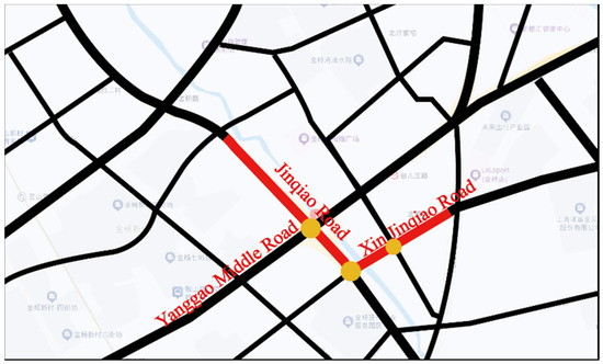
Figure 8.
Geographic location map of coordinated intersections.
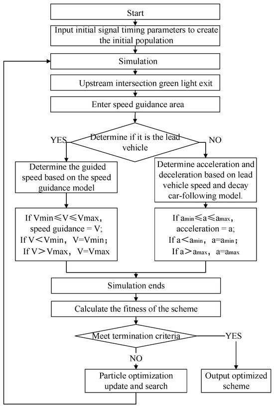
Figure 9.
Model solution and simulation flowchart.
Table 5.
Current signal timing schemes for each intersection.
Table 6.
Traffic survey results of each intersection.
The following are the experimental steps for the entire case analysis:
- Solution of Case Coordination Control Scheme: According to the surveyed data, they are substituted into the speed guidance coordination control model established in this paper for a solution to obtain the operation scheme of speed guidance coordination control. The specific steps are shown in Section 4.1.
- Simulation Verification: A VISSIM simulation platform is built, simulation parameters are set, and the effect of the speed guidance coordination control scheme implemented on the coordination path is verified. The specific steps are shown in Section 4.2.
- Result Analysis: Data analysis and comparison are conducted on the experimental data obtained after simulation. The specific steps are shown in Section 4.3.
Green Time: The duration during which the traffic light shows green, during which vehicles in the corresponding direction are allowed to pass.
Red Time: The duration during which the traffic light shows red, during which vehicles in the corresponding direction are prohibited from passing.
Yellow Time: A short transitional period when the traffic light shows yellow, which occurs after the green light ends and before the red light starts.
All-Red Time: A short period when traffic lights in all directions show red simultaneously, usually occurring during the gap of phase switching.
EW-TH represents the east–west through-traffic flow.
EW-LT represents the east–west left-turn traffic flow.
NS-TH represents the north–south through-traffic flow.
NS-LT represents the north–south left-turn traffic f low.
Vehicles are classified according to the turning left behavior, going straight behavior, and turning right behavior that they are prepared to take when entering the intersection.
4.1. Solution Approach
The multi-objective coordination control scheme proposed in this paper is applied to optimize the signal timing plans of the intersection. The particle swarm optimization (PSO) method is used to calculate the multi-objective function with a maximum iteration number n = 100, population size m = 200, and inertia weight of 0.5, and both learning factors and are set to 1. Subsequently, the intersection is simulated in VISSIM based on the current signal timing plan. Then, VISSIM simulations are conducted for both the left-turn coordination control model without speed guidance and the left-turn coordination control model with speed guidance. The solution steps and simulation verification process are shown in the flowchart.
During the optimization process, the survey data was processed to obtain the input values of various parameters, as shown in Table 7.
Table 7.
Model input parameter values.
Based on the characteristics of urban traffic flow and the actual observed data, the speed range of the road section is set to between 40 km/h and 55 km/, so , . In addition, the speed variation between adjacent road sections should not be too large. Therefore, the speed range is set to and the values of the upper and lower green wave bandwidth, road section travel time, phase difference between intersections, and total cycle are solved and shown in Table 8.
Table 8.
Model calculation results.
4.2. Simulation Parameter Settings
This study establishes a VISSIM simulation platform to validate the optimization effectiveness of the coordinated control scheme. The specific simulation parameter configurations are as follows:
- (1)
- Road geometric parameters: The basic path parameters are set according to the number of lanes, lane width, and intersection layout obtained through field surveys, measurements, and statistics.
- (2)
- The traffic flow composition parameter settings are shown in Table 9.
Table 9. Traffic flow composition parameters.
- (3)
- The simulation operation parameter settings are shown in Table 10.
Table 10. The simulation operation parameters.
4.3. Results Analysis
After calculating the cycle duration based on the AM-BAND model, the signal timing for each intersection is adjusted. The yellow light time and all-red time for each phase are set to 3 s and 2 s, respectively. A comparison is made between the original timing scheme and the multi-objective optimization model’s timing scheme without speed guidance. The comparison results of each objective value before and after optimization are shown in the Table 11.
Table 11.
Signal timing models before and after optimization for each intersection.
Using VISSIM for simulation, the simulation parameters are set as follows: the simulation period is 3600 s, the simulation step size is 1 s, and the random seed is set to 50. Considering the instability during the initial phase of the simulation, the first 300 s are treated as a warm-up period. The simulation output data from 300 to 3600 s is used for evaluation. The evaluation results for the main intersections are shown in the Table 12.
Table 12.
Simulation results for main intersections under different schemes.
By analyzing the evaluation indicators for the main intersections, it can be seen that, from an overall optimization perspective, both the no speed guidance model and the left-turn coordination control model under speed guidance show some improvement compared to the traditional coordination control model. Compared to the traditional coordination control model, the no speed guidance model reduces the average vehicle delay by 6.82%, queue length by 3.44%, and average number of stops by 0.09%. Furthermore, with the introduction of speed guidance, the model further reduces the average vehicle delay, queue length, and number of stops by 16.91%, 8.59%, and 13.84%, respectively. However, from the perspective of individual intersections, the no speed guidance multi-objective coordination optimization model shows an increase in delay, queue length, and number of stops at the left-turn coordination intersection (Jinqiao Road—Xin Jinqiao Road). This may be due to the coordinated left-turn green light time, which causes delays and stops in other directions.
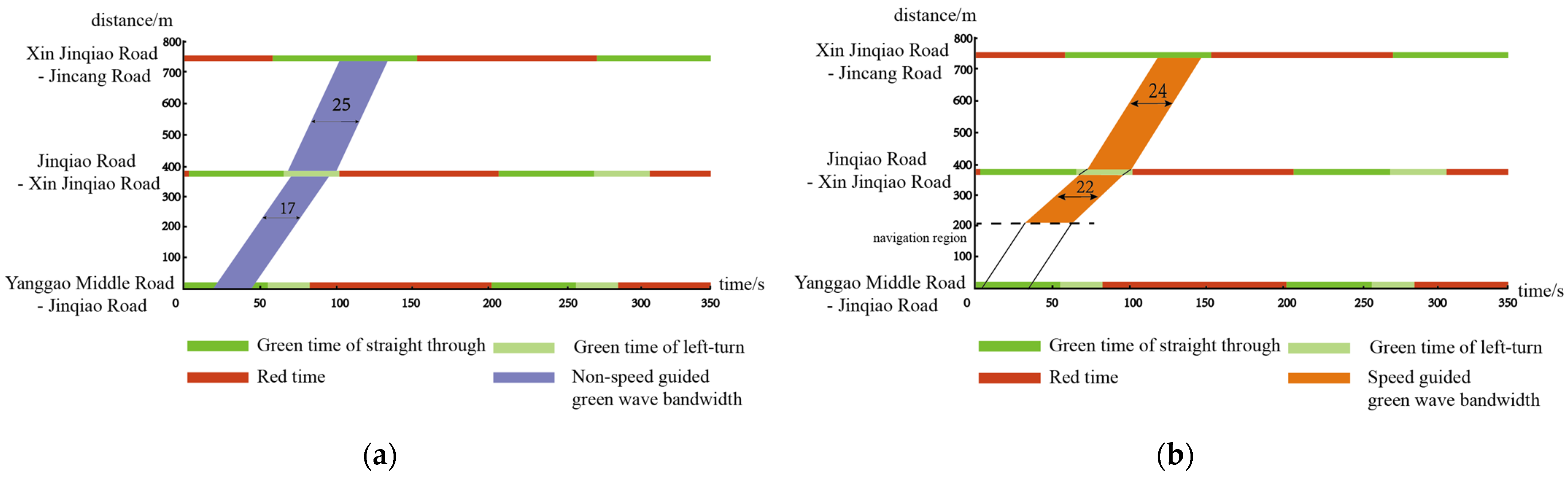
To further analyze the optimization effect of the left-turn coordination path under different schemes, the path simulation results were evaluated, and the green wave time–distance diagram is shown in the Figure 10. The speeds for each stage under left-turn speed guidance are as follows: pre-left-turn straight-phase speed 11.3 m/s → left-turn-phase speed 10.05 m/s → post-left-turn straight-phase speed 13.4 m/s. The left-turn-phase speed (10.05 m/s) is influenced by the left-turn acceleration decay and the turning radius, and it is lower than the minimum speed constraint. The evaluation results for the path are shown in the Table 13 and Table 14.

Figure 10.
(a) Non-speed guidance green wave bandwidth spatiotemporal diagram; (b) speed guidance-based spatiotemporal diagram of green wave bandwidth.
Table 13.
Left-turn coordination control path simulation results.
Table 14.
Comparison of path optimization results for each model.
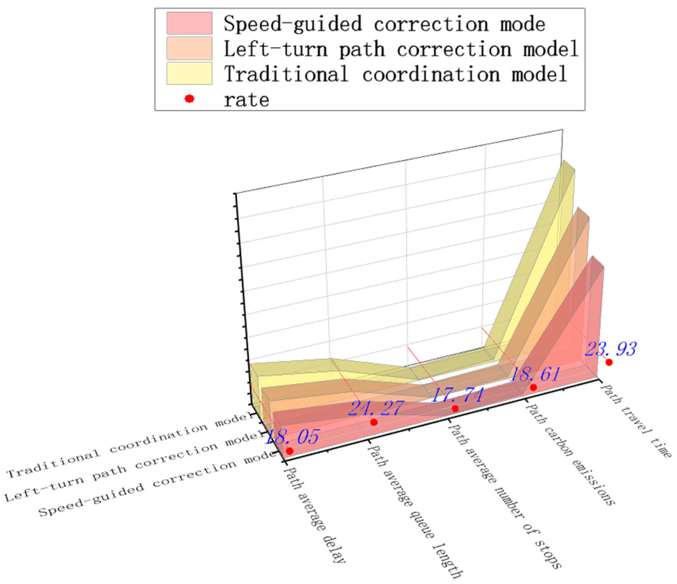
From the perspective of the green wave bandwidth, the path coordination correction model considering left turns increased the green wave bandwidth by 16.67% compared to the traditional coordination model (hereafter referred to as the “correction model”). Furthermore, with the introduction of speed guidance for left turns, the green wave bandwidth increased by another 9.52%. The increase in the green wave bandwidth effectively shortened vehicles’ travel time and the average delay per vehicle. Compared to the traditional model, the correction model reduced the travel time by 6.49% and the average delay per vehicle by 6.57%. With the further addition of speed guidance, the travel time was reduced by 18.65% and the average delay per vehicle was reduced by 12.77%. The result is shown in the Figure 11.
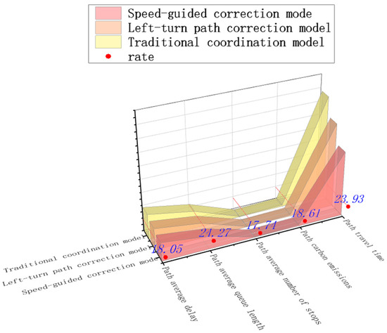
Figure 11.
Optimization results of each model.
From the perspective of carbon emissions, the correction model can effectively reduce carbon emissions. Compared to the traditional coordination model, its emissions were reduced by 12.99%. Further consideration of speed guidance for left turns results in an additional reduction of 6.47% in carbon emissions. The decrease in carbon emissions is mainly due to the reduction in the vehicle queue length and the number of stops along the path. Compared to the traditional model, the correction model reduced the queue length by 9.78% and the number of stops by 4.84%. With the further addition of speed guidance, the queue length was reduced by 16.06% and the number of stops was reduced by 13.56%. The result is shown in the Figure 11.
In summary, the left-turn coordination control model with speed guidance proposed in this paper can provide accurate driving speeds for left-turning vehicles, effectively improving the commuting efficiency of the left-turn path.
5. Conclusions
This study proposes a multi-objective optimization model for coordinated left-turn path control under speed guidance to achieve the coordinated management of and speed guidance for left-turning traffic, which can be applied to the coordinated induction control of urban commuter traffic, with the main contributions as follows:
- (1)
- By integrating acceleration/deceleration characteristics and turning radius effects into the traditional FVD model, we developed an acceleration attenuation car-following model for left-turning vehicles approaching intersections;
- (2)
- Additionally, by incorporating the minimum-jerk principle and the trajectory characteristics of vehicles at left-turn intersections, a speed guidance strategy was proposed for vehicles on paths that include left-turn directions;
- (3)
- By integrating left-turn speed guidance with a multi-objective optimization approach, a multi-objective optimization model for the coordinated control of left-turn paths under speed guidance was proposed. The model aims to maximize the total intersection bandwidth and minimize the carbon emissions of path vehicles while simultaneously optimizing vehicle guidance speed and intersection signal timing. This achieves the coordinated control and optimization of left-turn paths;
- (4)
- Considering the multidimensional characteristics of the model’s decision variables, a simulation platform was built using VISSIM. Taking three consecutive intersections in the Jinse Central Ring area of Pudong New District, Shanghai, as examples, the model was validated through simulation. The results show that compared to the traditional coordinated control model, the left-turn coordinated control model with speed guidance increases the total green wave bandwidth by 27.78% and reduces carbon emissions by 18.61%. Compared to the multi-objective optimization model without speed guidance, the total green wave bandwidth increases by 9.52%, while carbon emissions decrease by 6.47%.
However, the current model does not incorporate signal-phase sequence optimization, instead relying on the phase sequences designed for through-traffic coordination to guide left-turn speed. This limitation compromises the effectiveness of the coordinated control and speed guidance model. Therefore, developing a left-turn speed guidance coordination control model with phase sequence optimization will be a key focus for future research.
Although this paper constructs an FVD vehicle-following model considering acceleration decay during left turns, the current verification mainly relies on the simulation platform (VISSIM). The model parameters depend on empirical assumptions, where the relationship between the sensitivity coefficients (k, λ) and turning radius is determined based on literature calibration and empirical formulas, lacking dynamic calibration and comparison with field data. Additionally, there is a lack of real vehicle data verification: parameters such as the assumed vehicle behavior, reaction time, and car-following behavior are all idealized settings, and error evaluation and parameter regression analysis have not been conducted using real fleet-following data.
Future field testing plans will focus on the practicality and accuracy of the model. It is planned to select 3 to 5 representative urban intersections for on-site testing, mainly including typical roads with high through- and left-turn traffic flows.
Author Contributions
Conceptualization, J.Y.; methodology, X.Z.; software, X.Z.; validation, X.Z. and C.Y.; formal analysis, X.Z.; investigation, X.Z. and C.Y.; resources, X.Z.; data curation, X.Z.; writing—original draft preparation, X.Z.; writing—review and editing, J.Y.; visualization, C.Y.; supervision, J.Y.; project administration, J.Y.; funding acquisition, J.Y. All authors have read and agreed to the published version of the manuscript.
Funding
This study was funded by the MOE (Ministry of Education in China), Project of Humanities and Social Sciences (22YJAZH131) “Research on mechanism of route coordinated control of commuter traffic at the urban road network in the environment of big data”.
Institutional Review Board Statement
Not applicable.
Informed Consent Statement
Not applicable.
Data Availability Statement
The data that support the findings of this study are available from the corresponding author, upon reasonable request.
Conflicts of Interest
The authors declare no conflict of interest.
References
- He, X.; Liu, H.X.; Liu, X. Optimal vehicle speed trajectory on a signalized arterial with consideration of queue. Transp. Res. Part C Emerg. Technol. 2015, 61, 106–120. [Google Scholar] [CrossRef]
- Chen, P.; Yan, C.; Sun, J.; Wang, Y.; Chen, S.; Li, K. Dynamic Eco-Driving Speed Guidance at Signalized Intersections: Multivehicle Driving Simulator Based Experimental Study. J. Adv. Transp. 2018, 2018, 6031764. [Google Scholar] [CrossRef]
- Liu, S.; Zhang, W.; Wu, X.; Feng, S.; Pei, X.; Yao, D. A simulation system and speed guidance algorithms for intersection traffic control using connected vehicle technology. Tsinghua Sci. Technol. 2019, 24, 160–170. [Google Scholar] [CrossRef]
- Niroumand, R.; Tajalli, M.; Hajibabai, L.; Hajbabaie, A. Joint optimization of vehicle-group trajectory and signal timing: Introducing the white phase for mixed-autonomy traffic stream. Transp. Res. Part C Emerg. Technol. 2020, 116, 102659. [Google Scholar] [CrossRef]
- Jing, B.B.; Lu, K.; Yan, X.W.; Wu, H.X.; Jian, M. A dual-cycle arterial green wave coordination control method based on speed guidance under vehicle-road cooperation. J. South China Univ. Technol. (Nat. Sci. Ed.) 2016, 44, 147–154. [Google Scholar]
- Xu, L.; Deng, M. Speed guidance method for signalized intersections based on vehicle-road cooperative environment. J. Transp. Inf. Saf. 2021, 39, 78–86. [Google Scholar]
- Shi, Q.; Chen, H.; Chen, Y. Research on speed guidance strategy for intelligent connected vehicle platoons at signalized intersections. J. Chongqing Jiaotong Univ. (Nat. Sci.) 2021, 40, 47–53. [Google Scholar]
- Shi, Q.; Qiu, Z.; He, S. Vehicle energy consumption optimization method based on speed guidance in a connected environment. J. Transp. Inf. Saf. 2023, 41, 138–146. [Google Scholar]
- Xu, B.; Ban, X.J.; Bian, Y.; Li, W.; Wang, J.; Li, S.E.; Li, K. Cooperative Method of Traffic Signal Optimization and Speed Control of Connected Vehicles at Isolated Intersections. IEEE Trans. Intell. Transp. Syst. 2019, 20, 1390–1403. [Google Scholar] [CrossRef]
- Zhang, J.; Li, Z.; Xing, G. Multi-objective optimization of dual-cycle arterial signal coordination control considering dynamic vehicle speed. J. Transp. Inf. Saf. 2021, 39, 60–67. [Google Scholar]
- Wang, X. Research on Optimization of Urban Arterial Signal Coordination Control Considering Vehicle Platoon Exhaust Emissions. Master’s Thesis, Beijing Jiaotong University, Beijing, China, 2017. [Google Scholar]
- Deng, M.; Hu, Y.; Li, X.; Xu, L. Arterial coordination optimization method based on speed guidance and actuated control. J. Syst. Simul. 2024, 36, 1309–1321. [Google Scholar]
- Xu, J.; Xiao, Y.; Jing, B.; Li, K. Green wave coordination control model for T-shaped intersections on arterial roads. Highw. Eng. 2018, 43, 78–81+133. [Google Scholar]
- Yang, X.; Li, T. Optimization of arterial coordination control and speed guidance considering left-turn merging. Control Theory Appl. 2023, 40, 1595–1601. [Google Scholar]
- Li, J. Modeling and Simulation of Connected Vehicle Car-Following with Acceleration Decay Under Unreliable Communication. Master’s Thesis, Beijing Jiaotong University, Beijing, China, 2023. [Google Scholar]
- Kesting, A.; Treiber, M. Calibrating Car-Following Models using Trajectory Data: Methodological Study. Transp. Res. Rec. J. Transp. Res. Board 2008, 2088, 148–156. [Google Scholar] [CrossRef]
- Wei, F.; Liu, P.; Chen, L.; Guo, Y.; Cai, Z. Modeling Car-Following Behavior of Left-Turning Vehicles at Signalized Intersections. Sci. Technol. Eng. 2020, 20, 7493–7498. [Google Scholar]
- Dias, C.; Iryo-Asano, M.; Abdullah, M.; Oguchi, T.; Alhajyaseen, W. Modeling Trajectories and Trajectory Variation of Turning Vehicles at Signalized Intersections. IEEE Access 2020, 8, 109821–109834. [Google Scholar] [CrossRef]
- Dias, C.; Iryo-Asano, M.; Oguchi, T. Predicting Optimal Trajectory of Left-Turning Vehicle at Signalized Intersection. Transp. Res. Procedia 2017, 21, 240–250. [Google Scholar] [CrossRef]
- Li, C.; Liu, X.; Rong, J. Development of Pavement Slipperiness Index and Its Application in Traffic Operation Management. J. Highw. Transp. Res. Dev. 2010, 27, 132–136+142. [Google Scholar]
- Zhang, C.; Xie, Y.; Gartner, N.H.; Stamatiadis, C.; Arsava, T. AM-Band: An Asymmetrical Multi-Band model for arterial traffic signal coordination. Transp. Res. Part C Emerg. Technol. 2015, 58, 515–531. [Google Scholar] [CrossRef]


Disclaimer/Publisher’s Note: The statements, opinions and data contained in all publications are solely those of the individual author(s) and contributor(s) and not of MDPI and/or the editor(s). MDPI and/or the editor(s) disclaim responsibility for any injury to people or property resulting from any ideas, methods, instructions or products referred to in the content. |
© 2025 by the authors. Licensee MDPI, Basel, Switzerland. This article is an open access article distributed under the terms and conditions of the Creative Commons Attribution (CC BY) license (https://creativecommons.org/licenses/by/4.0/).