Abstract
Our society is facing serious challenges from global warming and environmental degradation. Scientists have identified carbon dioxide as one of the causes. Our society is embracing carbon offset as a way to field the challenges. The purpose of carbon offset is trying to cancel out the large amounts of carbon dioxide by investing in projects that reduce or remove emissions elsewhere. Examples of carbon offset projects are planting trees, renewable energy projects, and capturing methane from landfills or farms. Not all carbon offset projects are equally effective. In stock markets, investors eagerly pursue carbon offset. Namely, investors favor carbon offset in addition to risk and return when investing. Therefore, investors supervise risk, return, and carbon offset. Investors’ pursuits raise the question of how to model carbon offset for investments. The traditional answer is to adopt carbon offset screening and engineer portfolios by stocks with good carbon offset ratings. However, Nobel Laureate Markowitz emphasizes portfolio selection rather than stock selection. Moreover, carbon offset is composed of multiple components, ranging from business, social, economic, and environmental aspects. This multifaceted nature requires more advanced models than carbon offset screening and portfolio selection. Within this context, we systematically formulate multiple-objective portfolio selection models that include carbon offset. Firstly, we extend portfolio selection and treat carbon offset as a whole. Secondly, we separate carbon offsets into different components and build models to monitor each component. Thirdly, we innovate a model to monitor each component’s expectation and mitigate each component’s risk. Lastly, we optimize the series of models and prove the models’ properties in theorems. Mathematically, this paper makes theoretical contributions to multiple-objective optimization, particularly by proving the consistency of efficient solutions during objective classification and model evolution, describing the structure of properly efficient sets for multiple quadratic objectives, and elucidating the optimization’s sensitivity analyses. Moreover, by coordinating the abstract objective function, our formulation is generalizable. Overall, this paper’s contribution is to model carbon offset investments through multiple-objective portfolio selection. This paper’s methodology is multiple-objective optimization. This paper’s achievements are to provide investors with greater precision and effectiveness than carbon offset screening and portfolio selection through engineering means and to mathematically prove the properties of the model.
Keywords:
decision making; multiple-objective optimization; portfolio selection; multiple-objective portfolio selection; carbon offset; risks MSC:
90C29; 91G10; 91G30
1. Introduction
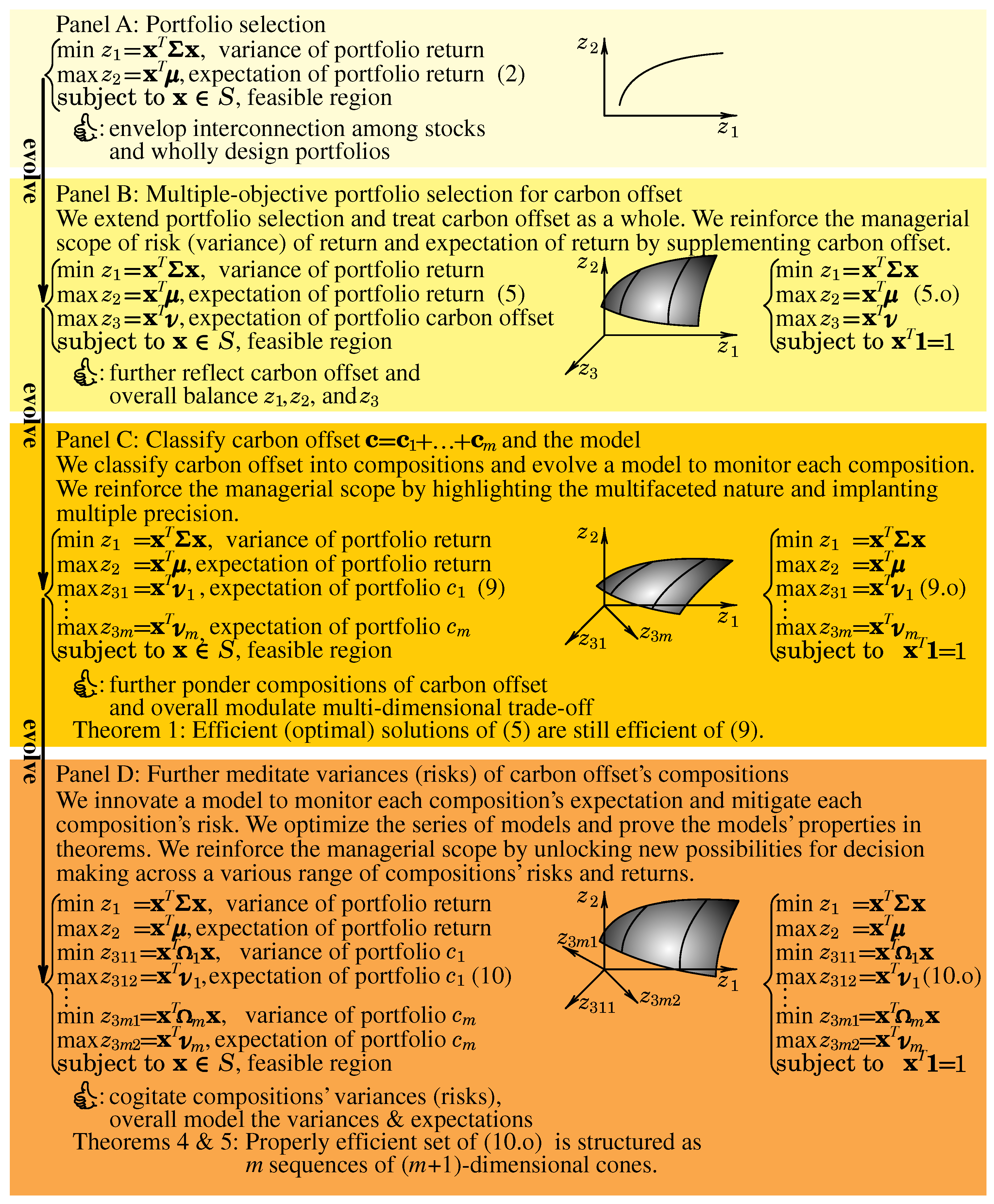
Figure 1 presents a “graphical abstract”, which is a visual summary of the main findings. It starts with Markowitz’s classical portfolio selection model. Then, this model is improved by adding several constraints and objectives that are connected with several carbon offset projects.
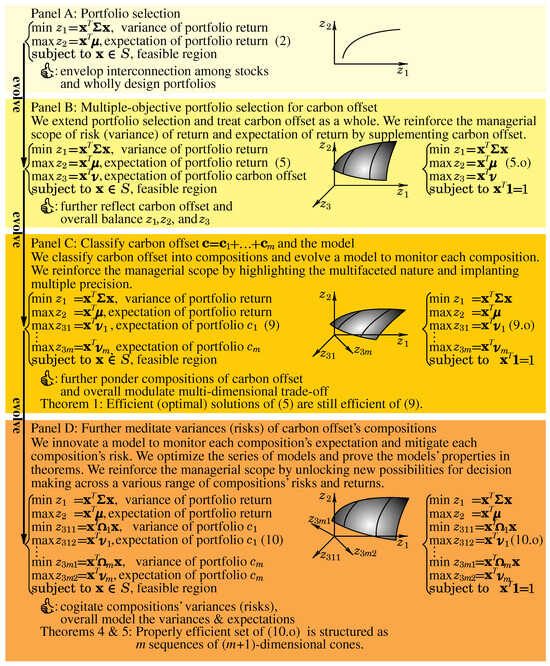
Figure 1.
Graphical abstract: It vertically contains four panels and horizontally contains three parts. We will elaborate on this in the Introduction.
The graphical summary consists of four vertical panels with progressively different shades, representing research progress, as follows:
- Panel A: portfolio selection;
- Panel B: multiple-objective portfolio selection for carbon offset;
- Panel C: classify carbon offset and the model; and
- Panel D: further meditate variances (risks) of carbon offset’s compositions.
The graphical abstract horizontally contains three parts as follows:
- Formulate and evolve (for the models and model evolution);
- Envisage (for the figures); and
- Optimize.
We will elaborate the graphical abstract in the following sections. We will explicitly refer to its stuffs by stating that, for instance, “Particularly in the “Formulate and evolve” part of Panel A of Figure 1, we depict Markowitz’s emphasis”.
1.1. Carbon Offset
Our society is facing serious challenges from global warming and environmental degradation. Scientists have identified carbon dioxide as one of the causes. Our society is embracing carbon offset to field the challenges.
Carbon offset refers to a way of compensating for carbon dioxide emissions—for example, from flying, driving, or manufacturing—by supporting projects that reduce or remove carbon dioxide elsewhere. In simple terms, we emit carbon dioxide in one place and pay to reduce or remove carbon dioxide somewhere else. Examples of carbon offset projects are planting trees, renewable energy projects, capturing methane from landfills or farms, improving energy efficiency in homes and businesses, helping individuals or companies cancel out their carbon footprint, and moving toward being carbon neutral (net zero emissions). As an important remark, not all carbon offset projects are equally effective. Some projects may be poorly managed or fail to deliver real emission reductions. Carbon offset should not replace efforts to reduce emissions at the source. Carbon offset is best used as a last step, not the first.
Researchers are actively investigating carbon offset. Huber et al. [1] analyzed the quality of carbon offset and contemplated the quality criteria for carbon offset. de Mello [2] surveyed voluntary carbon offset programs in aviation. Wei et al. [3] explored the research advancement of carbon offset by a bibliometric measure. Hyams and Fawcett [4] exposed the ethical basis for carbon offset and assessed empirical disagreements. González-Ramírez et al. [5] reviewed the design and implementation of carbon offset in agriculture. Lovell [6] overviewed the governance of carbon offset markets and commenced implications for governance structures.
1.2. The Urgency to Engineer Carbon Offset Investments by Multiple-Objective Portfolio Selection in Stock Markets
In stock markets, investors eagerly pursue carbon offset in investments1. The pursuit raises the question how to model carbon offset for investments.
The traditional answer is to adopt carbon offset screening and build portfolios by stocks with good carbon offset ratings. However, Markowitz [7] (p. 3) emphasized portfolio selection rather than stock selection, because portfolio selection and its extensions envelop the interconnection among stocks and wholly design portfolios, while stock selection does not. Particularly in the “Formulate and evolve” part of Panel A of Figure 1, we depict Markowitz’s emphasis.
Moreover, carbon offset is composed of multiple compositions including business, social, economic, and environmental aspects. This multifaceted nature requires more advanced models than carbon offset screening and portfolio selection.
Within this context, we systematically formulate carbon offset investments by multiple-objective portfolio selection. Firstly, we treat carbon offset as a whole and extend portfolio selection. Secondly, we classify carbon offset into compositions and evolve a model to monitor each composition. Thirdly, we innovate a model to monitor each composition’s expectation and mitigate each composition’s risk. Lastly, we optimize the series of models and prove the models’ properties in theorems.
1.3. Portfolio Selection as the Birth of Modern Finance
Portfolio selection is universally recognized as the birth of modern finance (as acclaimed by Rubinstein [8] (p. 1041)). Markowitz [9] presumed the vector of the returns of n stocks as (as a random vector). For a portfolio weight vector , Markowitz [9] calculated the portfolio return r (as a random variable) as follows:
For notations, normal symbols (e.g., r) denote scalars. Bold-face symbols (e.g., or ) denote vectors or matrices. Please note the difference between r (portfolio return as a scalar) and (stock returns as a vector). We introduce numerous symbols and will list the symbols in the Appendix.
Markowitz [7] (p. 6) accentuated both risk and return. Markowitz [9] (p. 83) originated portfolio selection as the following two-objective optimization2:
where is the covariance matrix of . is a vector of the expectations of stock returns (i.e., . A portfolio is fixed by its weight vector . measures the variance of r and thus indicates risk. measures the expectation of r and thus indicates return. is a feasible region.
(2) is a model of two-objective optimization, and investors simultaneously minimize the variance of portfolio return and maximize the expectation of portfolio return. We will review multiple-objective optimization in Section 2. In contrast, ordinary optimization optimizes only one objective function. The optimal result of (2) in space is called an efficient frontier. Particularly in the “Formulate and evolve” part of Panel A of Figure 1, we depict (2). Particularly in the “Envisage” part of Panel A of Figure 1, we depict an efficient frontier.
1.4. The Rise of Multiple-Objective Portfolio Selection as Extensions of Portfolio Selection
Markowitz [11] (pp. 471 and 476) realized extra objectives after his feat (2). So did Sharpe [12]. Markowitz [13] analyzed short-run portfolio variance and long-run portfolio variance. Fama [14] (pp. 445–447) and Cochrane [15] (pp. 1081–1082) used multiple factors for asset pricing models. Harvey and Siddique [16] considered skewness. Lo et al. [17] inspected liquidity. Pedersen et al. [18] treated ESG. Chow [19] studied tracking errors.
Ehrgott et al. [20], Steuer et al. [21], Dorfleitner et al. [22], Hirschberger et al. [23], Utz et al. [24], Qi et al. [25], Qi and Steuer [26], and Utz and Steuer [27] extended (2) and proposed multiple-objective portfolio selection as follows:
where are vectors of the expectations of general stock objectives (e.g., carbon offset). measure the expectations of general portfolio objectives.
Spronk and Hallerbach [28], Bana e Costa and Soares [29], Steuer and Na [30], Zopounidis et al. [31], Aouni et al. [32], and La Torre et al. [33] surveyed the area.
1.5. Theoretical Originality and Practical Contribution
1.5.1. Overall Originality and Contribution
Mathematically, this paper makes theoretical contributions to multiple-objective optimization, particularly by proving the consistency of efficient solutions during objective classification and model evolution, describing the structure of properly efficient sets for multiple quadratic objectives, and elucidating the optimization’s sensitivity analyses. Practically, this paper enriches investments for carbon offset. “Systematically” in the title epitomizes integrally formulating, classifying, evolving, and optimizing a series of models. We crystalize the originality and contribution in the following sections.
1.5.2. Formulating
The carbon offset of a corporation typically changes from year to year and thus acts as a random variable. The carbon offsets of n corporations or stocks also change from year to year and thus act as a random vector. We denote the vector of carbon offsets of the n stocks as (as an vector). For a portfolio weight vector (as an vector), we follow (1) and calculate the portfolio carbon offset c (as a random variable) as follows3:
For example, for stocks, we presume with entries as follows:
For , we compute portfolio carbon offset as follows:
We extend the classical portfolio selection model that is model (2) by proposing a multi-objective model with three objective functions: minimize the variance of the portfolio return, maximize the expected portfolio return and maximize the expected portfolio carbon offset return.
where is a vector of the expectations of stock carbon offsets (i.e., . measures the expectation of c. Steuer et al. [21] (pp. 302–303) justified (5). Particularly in the “Formulate and evolve” part of Panel B of Figure 1, we depict (5).
The optimal result of (5) in space extends into a surface (from an efficient frontier as depicted in the “Envisage” part of Panel A of Figure 1). Particularly in the “Envisage” part of Panel B of Figure 1, we depict such a surface. The surface acts as a panorama of the optimal variance of portfolio return (), expectation of portfolio return (), and expectation of portfolio carbon offset (). Investors further reflect carbon offset and overall balance , , and on the surface. Particularly in the “Formulate and evolve” part of Panel B of Figure 1, we depict the advantage.
1.5.3. Classifying
Carbon offset is composed of multiple compositions (e.g., carbon dioxide control and pollutant control) including business, social, economic, and environmental aspects. We acknowledge the multifaceted nature of these compositions and formulate to control each composition. We further presume that carbon offset is composed of m compositions as follows:
In Section 1.5.2, we denote the vector of carbon offset of the n stocks as (as an vector). Here, still of the n stocks, is an vector, and is an vector. We will illustrate in (8).
After presuming the n stocks’ carbon offset compositions, we compute a portfolio’s carbon offset compositions.
- In (4), for the vector of carbon offsets of the n stocks as (as an vector) and a portfolio weight vector (as an vector), we calculate the portfolio carbon offset c (as a scalar).
- Similarly, for the vector of carbon offset’s first compositions of the n stocks as (as an vector) and a portfolio weight vector (as an vector), we follow (4) and calculate the portfolio (as a scalar) as follows:
For example, for stocks, we simply presume that carbon offset is composed of carbon dioxide control and pollutant control alone as follows:
With a portfolio weight vector , we total the portfolio carbon dioxide control and portfolio pollutant control as follows:
By (6) and (7), we refine (5), classify carbon offset into the compositions, control each composition, and instigate the following model:
where … are vectors of the expectations of stock … (i.e., , …, ). By (9), investors simultaneously minimize the variance of portfolio return, maximize the expectation of portfolio return, maximize the expectation of portfolio , and maximize the expectation of portfolio . To maintain consistency of symbol usage, we deploy symbols … (instead of …). Steuer et al. [21] (pp. 302–303) justified (9). Particularly in the “Formulate and evolve” part of Panel C of Figure 1, we depict (9).
The optimal result of (9) in space again extends into a surface (from a surface as depicted in the “Envisage” part of Panel B of Figure 1). Particularly in the “Envisage” part of Panel C of Figure 1, we depict such a surface. Our depiction is hypothetical because we engage in -dimensional space, which resists visualization. The surface acts as a panorama of the optimal . Investors further ponder the compositions of carbon offset and overall modulate the -dimensional trade-off on the surface. Particularly in the “Formulate and evolve” part of Panel C of Figure 1, we depict the advantage.
1.5.4. Evolving
Furthermore, we reinforce (9) and evolve the following model:
where … are covariance matrices of … of (6), respectively. By (10), investors simultaneously minimize the variance of portfolio return, maximize the expectation of portfolio return, minimize the variance of portfolio , maximize the expectation of portfolio , minimize the variance of portfolio , and maximize the expectation of portfolio . Qi and Steuer [34] (pp. 1579–1581) justified (10). Particularly in the “Formulate and evolve” part of Panel D of Figure 1, we depict (10).
The optimal result of (10) in space further extends into a surface (from a surface as depicted in the “Envisage” part of Panel C of Figure 1). Particularly in the “Envisage” part of Panel D of Figure 1, we depict such a surface. Our depiction is hypothetical because we engage in -dimensional space, which resists visualization. The surface acts as a panorama of the optimal . Investors cogitate the compositions’ variances (risks) and overall model the pairs of variances and expectations on the surface. Particularly in the “Formulate and evolve” part of Panel D of Figure 1, we depict the advantage.
1.5.5. Optimizing
Even (5) alone is complex. There does not exist public domain software despite promising algorithms. (9) and (10) are much more complex than (5)5. We operationalize (5), (9), and (10) by simplifying as and functioning the following models:
where is the vector with all entries equal to one.
Particularly in the “Optimize” parts of Panels B, C, and D of Figure 1, we depict (5.o), (9.o), and (10.o), respectively.
1.6. Paper Structure
The rest of this paper is organized as follows: We review portfolio selection and multiple-objective optimization in Section 2. We explicate (5), (9), and (10) and prove the consistency of efficient solutions from (5) to (9) in Section 3. We optimize (5.o), (9.o), and (10.o) and prove the structure of the properly efficient set of (10.o) in Section 4. We illustrate in Section 5. We discuss and conclude in Section 6. We list major symbols in Appendix A.
2. Theoretical Background: Multiple-Objective Optimization and Portfolio Optimization
In this section, we review multiple-objective optimization, multiple-objective portfolio optimization, and investments in carbon offset.
2.1. Multiple-Objective Optimization
Scholars (e.g., Steuer [10]) formalized multiple-objective optimization as follows:
where is a decision vector in decision space. k is the number of objectives. are objective functions. is a criterion vector in criterion space. is a feasible region in decision space. is the feasible region in criterion space. Scientists launch the following definitions:
Definition 1.
For and , that dominates is defined as with at least one strict inequality.
Definition 2.
That is nondominated is defined as that there does not exist a such that dominates . Then, if is an inverse image of (i.e., ), is efficient.
Definition 3.
That is properly efficient is defined as that is efficient and there exists a scalar such that for each , for some such that whenever and . Then, if is the criterion vector of , is properly nondominated.
One purpose of multiple-objective optimization is to ascertain the following:
- Set of efficient decision vectors as an efficient set (denoted as E);
- Set of nondominated criterion vectors as a nondominated set (denoted as N);
- Set of properly efficient decision vectors as a properly efficient set; and
- Set of properly nondominated criterion vectors as a properly nondominated set.
For terminologies, Markowitz [9] specified the optimal result of (2) in space as an efficient frontier. Contrarily, we respect Definition 2, reserve “nondominated” for criterion space and “efficient” for decision space, and specify the result as a nondominated set.
To resolve (11), researchers (e.g., Steuer [10] (pp. 202–205)) often harnessed e-constraint methods as follows:
where … are the parameters. (12) is an ordinary one-objective optimization. Researchers often presume a set of …, solve (12) with the set of …, and presume that the optimal decision vectors of (12) are as efficient as those of (11). However, Steuer [10] (p. 203) warned that e-constraint methods are ad hoc and can actually locate inefficient decision vectors of (11).
To resolve (11), researchers (e.g., Steuer [10] (pp. 165–168)) also often harnessed weighted-sums methods as follows:
where , …, but are the parameters. Researchers often presume a set of …, crack (13) with the set of …, and presume the optimal decision vectors of (13) as efficient of (11). However, Qi [35] (pp. 1683–1685) argued that presuming an appropriate set of … is tricky, but Qi [35] (pp. 1683–1685) experimented merely with the optimization for (2).
2.2. Multiple-Objective Portfolio Optimization
2.2.1. Analytical Methods
Sharpe [36] (pp. 59–62) and Merton [37] contemplated
They analytically derived the efficient set. “Analytical” means closed-form formulae. By analyticity, the computational complexity of Sharpe [36] (pp. 59–62) and Merton [37] was very low. Sharpe [38] anchored his capital asset pricing model on (14). However, Merton [37] and Sharpe [38] did not ponder the general feasible region S of (2) and thus sacrificed generality for analyticity. Huang and Litzenberger [39] (p. 60) endorsed (14) for its analyticity and empirical implications.
Qi et al. [25] extended (14), inserted one linear objective function, and also analytically derived the efficient set. However, Qi et al. [25] did not ponder the general feasible region S of (2) and thus sacrificed generality for analyticity. Qi and Steuer [26] extended the research of Qi et al. [25], inserted more linear objective functions and equality constraints, and also analytically derived the efficient set. Qi and Steuer [34] extended the research of Qi and Steuer [26], inserted more quadratic objective functions, and also analytically derived the properly efficient set. Although Qi and Steuer [26] and Qi and Steuer [34] admitted more equality constraints than Qi et al. [25], Qi and Steuer [26] and Qi and Steuer [34] were still confined to the feasible regions formed by equality constraints only. By analyticity, the computational complexity of Qi et al. [25], Qi and Steuer [26], and Qi and Steuer [34] was very low.
2.2.2. Repetitive Quadratic Programming
Scholars (e.g., Bodie et al. [40] (pp. 230–242)) employed e-constraint methods or weighted-sums methods to (11) and obtained discrete approximation of the nondominated set of (11). Because the scholars repetitively solve quadratic programming problems with established software (e.g., Matlab), the complexity was medium.
2.2.3. Parametric Quadratic Programming
To crack (2), Markowitz [41] and Markowitz and Todd [42] employed parametric quadratic programming and gained the full and precise efficient set6. For general three-objective portfolio selection, Hirschberger et al. [23] also employed parametric quadratic programming and gained the full and precise efficient set. Goh and Yang [44], Jayasekara et al. [45], and Jayasekara et al. [46] also designed parametric quadratic programming algorithms.
Markowitz [41], Markowitz and Todd [42], and Hirschberger et al. [23] exploited the properties of the efficient set (e.g., the efficient set’s connectedness) and started the algorithms with a linear programming problem; the complexity of the algorithms was relatively low. However, Markowitz [41], Markowitz and Todd [42], and Hirschberger et al. [23] operated advanced theory of parametric optimization, so the algorithms were elusive.
Unfortunately, there does not exist public domain software for general multiple-objective portfolio selection, so investors still cannot execute it. To the best of our knowledge, even for merely three-objective portfolio selection, only Hirschberger et al. [23] coded the algorithm, but the code is still private.
2.2.4. Heuristic Methods
Heuristic methods can handle additional nonlinear formulations and thus become important provisional tools. For instance, Deb [47] exhibited evolutionary algorithms. The complexity of evolutionary algorithms can be maximally medium.
2.2.5. Other Latest Methods
Additionally, scientists are advancing other latest methods. For instance, Goli and Tirkolaee [48] promisingly designed a closed-loop supply chain network, accelerated the Benders decomposition algorithm and optimized product portfolio design models but did not generalize for more objective models. Tirkolaee [49] scrutinized novel possibilistic multi-objective mixed-integer linear programming models for sustainable and reliable waste management system design and performed sensitivity analyses but did not prove mathematical properties in theorems. Biswas et al. [50] meditated robust mathematical models for resource allocation and logistics for COVID-19 and hosted a group of late optimization techniques but did not prove mathematical properties in theorems.
2.3. Investments for Carbon Offset
To the best of our knowledge, there exists a limited amount of research for investments in carbon offset. Lou et al. [51] sampled 534 carbon offset projects and identified corporate motivations for carbon offset investments but did not prescribe models for a mass of investors. Lee [52] determined the optimum for investing in carbon emissions reduction by EOQ models and compared regulations for corporate total cost and carbon footprint but did not prescribe models for a mass of investors. Ngilangwa [53] explored the motivation for corporations to invest in carbon offset and contended compliance to the environmental regulations as the major motivation but did not prescribe models for a mass of investors.
3. Formulation and Evolution
3.1. Further Justifying and Illuminating (5)
For portfolio selection (2) and multiple-objective portfolio selection (5) (as an extension), we illuminate the feasible regions, efficient sets, nondominated sets, and advantage of (5) in Figure 2.
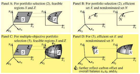
In Panel A of Figure 2, we depict the feasible regions S and Z (as reviewed in Section 2) of (2) as shaded regions. Our depiction of S is hypothetical because we engage in n-dimensional space , which resists visualization. Portfolio selection (2) maps S to Z. We depict and .
In Panel B of Figure 2, we depict the efficient set E and nondominated set N of (2). (2) maps E to N. We depict .
In Panel C of Figure 2, we depict the S and Z of (5) as shaded regions. (5) maps S to Z. We depict and . The feasible regions S of (2) and (5) are identical. The Z of (5) extends from a two-dimensional set into a three-dimensional set, because investors integrally reflect the variance of portfolio return, expectation of portfolio return, and expectation of portfolio carbon offset. Contrarily, the investors of (2) simultaneously consider merely the variance of portfolio return and expectation of portfolio return.
In Panel D of Figure 2, we depict the E and N of (5). (5) maps E to N. We depict . The N of (5) extends from a two-dimensional set into a three-dimensional set. The N acts as a panorama of the optimal variance of portfolio return, expectation of portfolio return, and expectation of portfolio carbon offset. Investors thus fully envisage the trade-offs and enjoy the freedom of choosing preferred portfolios on N.
3.2. Proving the Consistency of Efficient Solutions from (5) to (9)
We deliberate the connection between (5) and (9) by proving the consistency of efficient solutions in the following lemma and theorem:
Theorem 1.
Proof.
For any efficient of (5), suppose that is not efficient for (9). Then, by Definition 2, there exists with the following relationship:
Because (19) and (20) all carry ≥, we add (19) and (20) and obtain as follows:
(5) and (9) possess identical S values. By (17), (18), (22), and (21), we infer that is not efficient for (5) because is more efficient than .
However, the inference contradicts the supposition. Therefore, the supposition is incorrect. Namely, is efficient for (9). Theorem 1 is proved. □
4. Optimization
4.1. Graphically Comparing Portfolio Optimization Methods
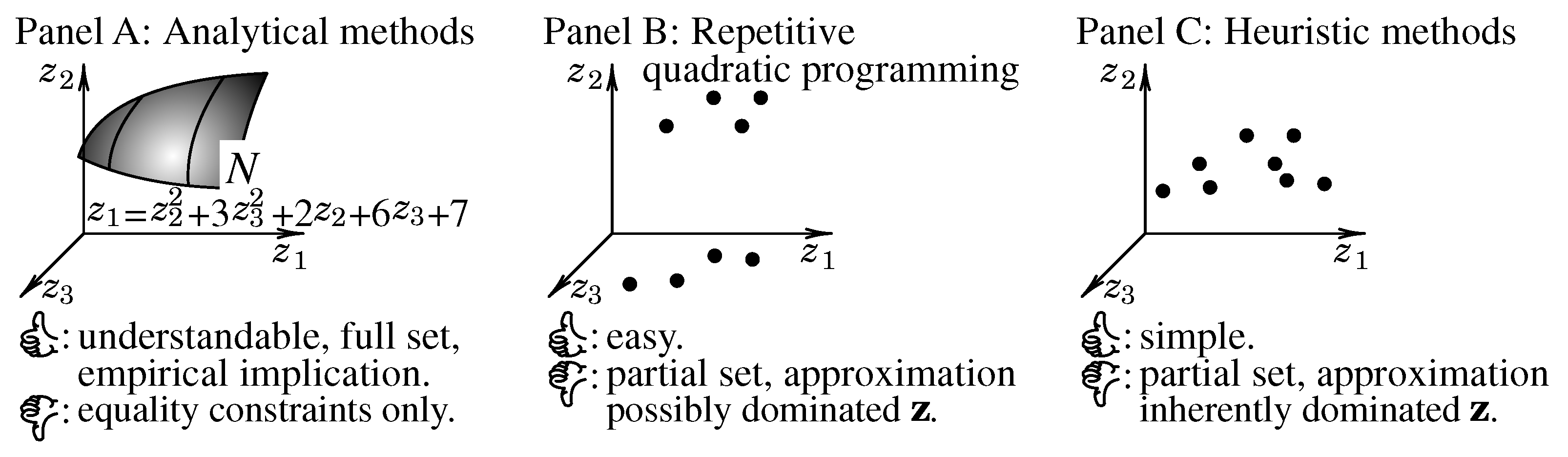
In Figure 3, we graphically compare optimization methods for (5.o), (9.o), and (10.o). Because public domain software for parametric quadratic programming does not exist, we exclude it for the comparison.
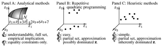
Figure 3.
Comparing portfolio optimization methods for (5.o), (9.o), and (10.o).
By analytical methods, Merton [37], Qi et al. [25], and Qi and Steuer [26] derived full nondominated sets. Moreover, the scholars prove the sets’ parabolic structure and paraboloidal structure, respectively. For instance, we depict a paraboloid in Panel A of Figure 3. Additionally, the scholars manipulate just calculus and linear algebra, so analytical methods are understandable. However, the disadvantage is that the scholars are confined to equality constraints only.
Repetitive quadratic programming is easy to execute. However, it renders only partial nondominated sets by discrete approximation. More importantly, it can render dominated criterion vectors (as depicted in Panel B of Figure 3).
Heuristic methods are simple to implement and can handle complex models. However, they inherently render dominated criterion vectors (as depicted in Panel C of Figure 3). Moreover, they also suffer from the disadvantage of repetitive quadratic programming.
4.2. Optimizing (5.o)
We inherit the following assumptions from Qi et al. [25]:
Assumption 1.
Σ is positive definite and thus invertible.
Assumption 2.
μ, ν, and 1 of (5.o) are linearly independent.
Geometrically, (23) is a two-dimensional translated cone. Namely, the cone is generated by and at the origin of and translated by . Moreover, the cone is closed because of and of (23). Mathematically, Qi et al. [25] (p. 171) proved the linear independence of and and structure of (23) in the following theorem:
Theorem 2.
The efficient set of (5.o) is structured as a two-dimensional cone.
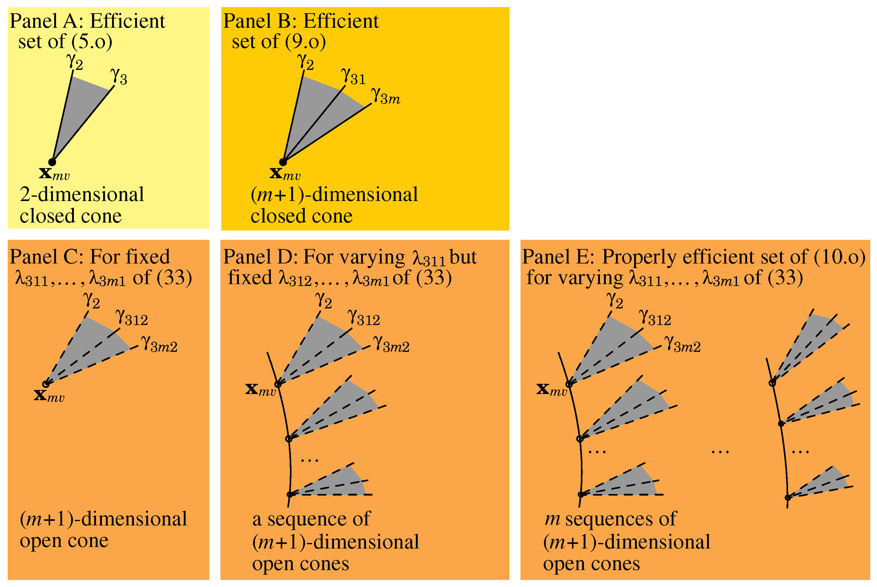
In Panel A of Figure 4, we show such a cone.
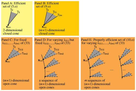
Figure 4.
The structure of the efficient sets of (5) and (9.o) and properly efficient of (10.o).
4.3. Optimizing (9.o)
We inherit the following assumption from Qi and Steuer [26].
Assumption 3.
μ, , …, , and are linearly independent.
By Qi and Steuer [26], we express the efficient set of (9.o) as follows:
where
Geometrically, (27) is an -dimensional translated cone. Namely, the cone is generated by , , …, at the origin of and translated by . Moreover, the cone is closed because of and … of (27). Mathematically, Qi and Steuer [26] (p. 532) proved the linear independence of , , …, and structure of (27) in the following theorem:
Theorem 3.
The efficient set of (9.o) is structured as an -dimensional cone.
In Panel B of Figure 4, we show such a cone.
4.4. Optimizing (10.o)
We inherit the following assumption from Qi and Steuer [34]:
Assumption 4.
… are positive definite and thus invertible.
By Qi and Steuer [34], we express the properly efficient set of (10.o) as follows:
where
Qi and Steuer [34] (p. 1582) proved of (33) as positive definite and thus invertible. Therefore, exists.
Geometrically, for fixed … of (33), (32) is a translated cone. Namely, the cone is generated by , , … at the origin of and translated by . Moreover, the cone is open because of and … of (32). Mathematically, we prove the cone as -dimensional in the following theorem and corollary:
Theorem 4.
Proof.
Suppose that there exist such that
where is the vector with all entries equal to zero. We substitute (35)–(37) into (38) and rearrange as follows:
By Assumption 3 and the existence of of (33), we premultiply , , …, , and by , and the products , , …, , and are also linearly independent as follows:
Proof.
The cone (32) is generated by , , …. , , … are linearly independent, so the cone is -dimensional. Corollary 1 is proved. □
In Panel C of Figure 4, we depict such a cone. We further reveal the structure of the properly efficient set of (10.o) in the following theorem:
Theorem 5.
For varying but fixed … of (33), (33) and (32) determine a sequence of -dimensional cones. For varying but fixed … of (33), (33) and (32) determine a sequence of -dimensional cones. Broadly, for varying … of (33), (33) and (32) determine m sequences of -dimensional cones. The m sequences of -dimensional cones describe the structure of the properly efficient set of (10.o).
Proof.
In Panel D of Figure 4, we depict a sequence of -dimensional cones for varying but fixed …. In Panel E, we depict m sequences of -dimensional cones for varying ….
4.5. Sensitivity Analyses
For the special case of … of (33), we deduce as follows:
The properly efficient set of (10.o) can subsume the efficient sets of (5.o) and (9.o). Therefore, we perform sensitivity analyses for only (10.o) as general cases.
For (10.o), the constraint is definitive, while the parameters (i.e., , , …, , , , …, ) can be indefinitive as follows:
We prove the following theorem for the sensitivity of (10.o). The theorem also holds for (5.o) and (9.o).
Theorem 6.
For (32), , , , …, are all nonlinearly sensitive with respect to Σ, , …, . Therefore, the sensitivity to Σ, , …, can be substantial. In contrast, is linearly sensitive with respect to μ. Therefore, the sensitivity to μ can be mild. is linearly sensitive with respect to . Therefore, the sensitivity to can be mild. …. is linearly sensitive with respect to . Therefore, the sensitivity to can be mild.
Proof.
, , …, all affect of (33). , , , …, all contain and thus are all nonlinearly sensitive with respect to , , …, . Because , , …, of (41) all can approach the status of singularity, while can vary dramatically. Therefore, the sensitivity to , , …, can be substantial.
of (35) contains and and thus is linearly sensitive with respect to . Therefore, the sensitivity to can be mild.
of (36) contains and and thus is linearly sensitive with respect to . Therefore, the sensitivity to can be mild.
of (37) contains and and thus is linearly sensitive with respect to . Therefore, the sensitivity to can be mild.
Theorem 6 is proved. □
5. Illustration
For four stocks, we simply adopt (8) and assume m = 2 compositions of carbon offset. We report the following parameters:
For (10.o), we would rather not report the computation of its properly efficient set, because we need to fix specific values for and .
6. Discussion
6.1. Practical, Theoretical, and Managerial Implications
Practically, this paper enriches investments for carbon offset. Investors can apply this paper, because investors can request some historical return and carbon offset data and readily channel the analyticity (as exhibited in Section 4). Classic finance organizations (e.g., Yahoo Finance) tender historical return data. Several carbon offset organizations (e.g., OPIS, a Dow Jones company) tender reports with data, and investors can design and extract carbon offset variables from the reports8. Academically, scholars (e.g., Bolton and Kacperczyk [54] and Yan et al. [55]) evaluated carbon offset and analyzed its effects.
Theoretically, this paper makes theoretical contributions for multiple-objective optimization, particularly by proving the consistency of efficient solutions during objective classification and model evolution, describing the structure of properly efficient sets for multiple quadratic objectives, and elucidating the optimization’s sensitivity analyses.
Managerially, this paper embraces data-driven modeling and evolves a series of models. Firstly, we extend portfolio selection and treat carbon offset as a whole. Therefore, we reinforce the managerial scope of risk (variance) of return and expectation of return by supplementing carbon offset. Secondly, we comprehend the various nature (e.g., business, social, economic, and environmental nature) of carbon offset, classify carbon offset into multiple compositions, and implant models for each composition. Therefore, we reinforce the managerial scope by highlighting the multifaceted nature and implanting multiple precision. Lastly, we evolve a model to monitor each composition’s risk (variance). Therefore, we reinforce the managerial scope by unlocking new possibilities for decision making across a various range of compositions’ risks and returns.
6.2. Generality of the Formulation
This paper’s formulation is general. Firstly, we regulate abstract compositions in (6) (instead of concrete and fixed compositions). Secondly, instead of concrete and fixed objective functions, we anchor the objective functions on the abstract compositions (e.g., in (9)). Lastly, even the orientation for carbon offset is exemplary. Namely, we can replace carbon offset by ESG, and the formulation and theorems (e.g., (9) and (10) and Theorems 4 and 5) still hold.
6.3. Future Directions
Overall, this paper’s contributions are to model carbon offset investments by multiple-objective portfolio selection. Mathematically, this paper makes theoretical contributions for multiple-objective optimization, particularly by proving the consistency of efficient solutions during objective classification and model evolution, describing the structure of properly efficient sets for multiple quadratic objectives, and elucidating the optimization’s sensitivity analyses.
Meanwhile, one crucial issue is that this paper lacks empirical testing using real market or carbon offset data. The use of real data could provide practical applicability. Therefore, we envision the following future directions: Firstly, we will dissect the limited research for rating carbon offset, design rating schemes, and tentatively rate component stocks of Dow Jones Industrial Average. To the best of our knowledge, such a rating is barely provided. Then, we maneuver this paper’s models and perform empirical testing.
Secondly, investors analytically foster the efficient sets and nondominated sets of (9), and (10). The nondominated sets are in high-dimensional spaces and reject visualization. Then, how do scholars advance algorithms to incorporate investors’ preferences and pin-point investors’ final portfolios?
Future work could focus on algorithm development, real-world testing, and user-oriented toolkits to bridge this gap.
Researchers are enriching multiple-objective optimization and arming carbon offset investors with systematic formulation.
Author Contributions
Conceptualization, L.L.; methodology, L.L.; software, L.L.; validation, Y.Q.; formal analysis, Y.Q.; investigation, L.L.; resources, Y.Q.; data curation, Y.Q.; writing—original draft preparation, L.L. and Y.Q.; visualization, Y.Q.; supervision, L.L.; project administration, L.L. All authors have read and agreed to the published version of the manuscript.
Funding
This research received no external funding.
Data Availability Statement
Data are available in a publicly accessible repository. The original data presented in the study are openly available in Mendeley Data at: https://data.mendeley.com/datasets/66dy7vnhpj/1 (accessed on 28 May 2025).
Acknowledgments
We would very much like to thank three anonymous referees for their highly constructive comments.
Conflicts of Interest
The authors declare no conflicts of interest.
Appendix A. Lists of Major Symbols and Meanings
Appendix A.1. English Symbols
- 1.
- is a vector, denotes the vector with all entries equal to one, and is introduced in (5.o).
- 2.
- is a vector, denotes the vector of carbon offset of the n stocks, and is introduced in (4).
- 3.
- c is a scalar, denotes the portfolio carbon offset, and is introduced in (4).
- 4.
- … are vectors, denote the vector of carbon offset’s first composition of the n stocks …the vector of carbon offset’s last composition of the n stocks, and are introduced in (6).
- 5.
- … are scalars, denote portfolio …portfolio , and are introduced in (7).
- 6.
- E is set, denotes the set of efficient decision vectors as efficient set, and is introduced in Section 2.1.
- 7.
- are scalars, denote objective functions, and are introduced in (11).
- 8.
- k is a scalar, denotes the number of objectives, and is introduced in (11).
- 9.
- N is set, denotes the set of nondominated criterion vectors as nondominated set, and is introduced in Section 2.1.
- 10.
- n is a scalar, denotes the number of stocks, and is introduced in Section 1.3.
- 11.
- is a random vector, denotes the return vector of n stocks, and is introduced in Section 1.3.
- 12.
- r is a random variable (random scalar), denotes portfolio return, and is introduced in (1).
- 13.
- 14.
- is an vector, denotes a portfolio weight vector, and is introduced in Section 1.3.
- 15.
- is a vector and is introduced in (24).
- 16.
- Z is a set, denotes the feasible region in criterion space, and is introduced in (11).
- 17.
- is a vector, denotes a criterion vector, and is introduced in (11).
- 18.
- is a scalar, denotes the variance of r, and is introduced in (2).
- 19.
- is a scalar, denotes the expectation of r, and is introduced in (2).
- 20.
- are scalars, denote the expectations of general portfolio objectives, and are introduced in (3).
- 21.
- … are scalars, denote the expectation of portfolio …the expectation of portfolio , and are introduced in (9).
- 22.
- … are scalars, denote the variance of portfolio …variance of portfolio , and are introduced in (10).
- 23.
- … are scalars, denote the expectation of portfolio …expectation of portfolio , and are introduced in (10).
Appendix A.2. Greek Symbols
- 1.
- is a vector and is introduced in (25).
- 2.
- is a vector and is introduced in (26).
- 3.
- is a vector and is introduced in (30).
- 4.
- is a vector and is introduced in (31).
- 5.
- is a vector and is introduced in (36).
- 6.
- is a vector and is introduced in (37).
- 7.
- is an vector, denotes the expectations of stock returns (i.e., , and is introduced in (2).
- 8.
- are vectors, denote vectors of the expectations of general stock objectives, and are introduced in (3).
- 9.
- is a vector, denotes the expectations of stock carbon offsets, and is introduced in (5).
- 10.
- … are vectors, denote the expectations of stock …, and are introduced in (9).
- 11.
- … are matrices, denote the covariance matrices of …, and are introduced in (10).
- 12.
- is an matrix, denotes the covariance matrix of , and is introduced in (2).
- 13.
- is a vector and is introduced in (33).
Notes
| 1 | Morgan Stanley predicts that voluntary carbon offset markets will advance from $2 billion in 2020 to $250 billion in 2050. Data source: “Where the Carbon Offset Market Is Poised to Surge”, Morgan Stanley. https://www.morganstanley.com/ideas/carbon-offset-market-growth (accessed on 1 March 2025). |
| 2 | Steuer [10] illuminated multiple-objective optimization. |
| 3 | Please note the difference between c (portfolio carbon offset as a scalar) and (stock carbon offsets as a vector). |
| 4 | Please note the difference between (portfolio level as a scalar) and (stock level as a vector). |
| 5 | We fantasize full and precise optimization (rather than partial and heuristic optimization) and will compare optimization methods in Section 4. |
| 6 | Pistikopoulos et al. [43] (pp. 6–7) defined parametric programming as optimization with parameters, while ordinary optimization (e.g., quadratic programming) carries no parameters. |
| 7 | By Assumption 1, we deduce , and is well-defined. |
| 8 | Data source: “Global Carbon Offsets Report”, OPIS, a Dow Jones company. https://www.opisnet.com/product/pricing/spot/carbon-offsets-report/ (accessed on 4 March 2025) |
References
- Huber, E.; Bach, V.; Finkbeiner, M. A qualitative meta-analysis of carbon offset quality criteria. J. Environ. Manag. 2024, 352, 119983. [Google Scholar] [CrossRef] [PubMed]
- de Mello, F.P. Voluntary carbon offset programs in aviation: A systematic literature review. Transp. Policy 2024, 147, 158–168. [Google Scholar] [CrossRef]
- Wei, J.; Zhao, K.; Zhang, L.; Yang, R.; Wang, M. Exploring development and evolutionary trends in carbon offset research: A bibliometric perspective. Environ. Sci. Pollut. 2021, 28, 18850–18869. [Google Scholar] [CrossRef] [PubMed]
- Hyams, K.; Fawcett, T. The ethics of carbon offsetting. WIREs Clim. Chang. 2013, 4, 91–98. [Google Scholar] [CrossRef]
- González-Ramírez, J.; Kling, C.L.; Valcu, A. An overview of carbon offsets from agriculture. Annu. Rev. Resour. Econ. 2012, 4, 145–160. [Google Scholar] [CrossRef]
- Lovell, H.C. Governing the carbon offset market. WIREs Clim. Chang. 2010, 1, 353–362. [Google Scholar] [CrossRef]
- Markowitz, H.M. Portfolio Selection: Efficient Diversification in Investments, 1st ed.; John Wiley & Sons: New York, NY, USA, 1959. [Google Scholar]
- Rubinstein, M. Markowitz’s “portfolio selection”: A fifty-year retrospective. J. Financ. 2002, 57, 1041–1045. [Google Scholar] [CrossRef]
- Markowitz, H.M. Portfolio Selection. J. Financ. 1952, 7, 77–91. [Google Scholar]
- Steuer, R.E. Multiple Criteria Optimization: Theory, Computation, and Application; John Wiley & Sons: New York, NY, USA, 1986. [Google Scholar]
- Markowitz, H.M. Foundations of portfolio selection. J. Financ. 1991, 46, 469–477. [Google Scholar] [CrossRef]
- Sharpe, W.F. Optimal Portfolios without Bounds on Holdings. Ph.D. Thesis, Graduate School of Business, Stanford University, Stanford, CA, USA, 2001. Available online: https://web.stanford.edu/~wfsharpe/mia/opt/mia_opt2.htm (accessed on 28 May 2025).
- Markowitz, H.M. How to represent mark-to-market possibilities with the general portfolio selection model. J. Portf. Manag. 2013, 39, 1–3. [Google Scholar] [CrossRef]
- Fama, E.F. Multifactor portfolio efficiency and multifactor asset pricing. J. Financ. Quant. Anal. 1996, 31, 441–465. [Google Scholar] [CrossRef]
- Cochrane, J.H. Presidential address: Discount rates. J. Financ. 2011, 66, 1047–1108. [Google Scholar] [CrossRef]
- Harvey, C.R.; Siddique, A. Conditional skewness in asset pricing tests. J. Financ. 2000, 55, 1263–1296. [Google Scholar] [CrossRef]
- Lo, A.W.; Petrov, C.; Wierzbicki, M. It’s 11pm—Do you know where your liquidity is? The mean-variance-liquidity frontier. J. Invest. Manag. 2003, 1, 55–93. [Google Scholar]
- Pedersen, L.H.; Fitzgibbons, S.; Pomorski, L. Responsible investing: The ESG-efficient frontier. J. Financ. Econ. 2021, 142, 572–597. [Google Scholar] [CrossRef]
- Chow, G. Portfolio selection based on return, risk, and relative performance. Financ. Anal. J. 1995, 51, 54–60. [Google Scholar] [CrossRef]
- Ehrgott, M.; Klamroth, K.; Schwehm, C. An MCDM Approach to Portfolio Optimization. Eur. J. Oper. Res. 2004, 155, 752–770. [Google Scholar] [CrossRef]
- Steuer, R.E.; Qi, Y.; Hirschberger, M. Suitable-portfolio investors, nondominated frontier sensitivity, and the effect of multiple objectives on standard portfolio selection. Ann. Oper. Res. 2007, 152, 297–317. [Google Scholar] [CrossRef]
- Dorfleitner, G.; Leidl, M.; Reeder, J. Theory of social returns in portfolio choice with application to microfinance. J. Asset Manag. 2012, 13, 384–400. [Google Scholar] [CrossRef]
- Hirschberger, M.; Steuer, R.E.; Utz, S.; Wimmer, M.; Qi, Y. Computing the nondominated surface in tri-criterion portfolio selection. Oper. Res. 2013, 61, 169–183. [Google Scholar] [CrossRef]
- Utz, S.; Wimmer, M.; Steuer, R.E. Tri-criterion modeling for constructing more-sustainable mutual funds. Eur. J. Oper. Res. 2015, 246, 331–338. [Google Scholar] [CrossRef]
- Qi, Y.; Steuer, R.E.; Wimmer, M. An analytical derivation of the efficient surface in portfolio selection with three criteria. Ann. Oper. Res. 2017, 251, 161–177. [Google Scholar] [CrossRef]
- Qi, Y.; Steuer, R.E. On the analytical derivation of efficient sets in quad-and-higher criterion portfolio selection. Ann. Oper. Res. 2020, 293, 521–538. [Google Scholar] [CrossRef]
- Utz, S.; Steuer, R.E. Empirical analysis of the trade-offs among risk, return, and climate risk in multi-criteria portfolio optimization. Ann. Oper. Res. 2024, Epub ahead of printing. [Google Scholar] [CrossRef]
- Spronk, J.; Hallerbach, W.G. Financial modelling: Where to go? With an illustration for portfolio management. Eur. J. Oper. Res. 1997, 99, 113–127. [Google Scholar] [CrossRef]
- Bana e Costa, C.A.; Soares, J.O. Multicriteria approaches for portfolio selection: An overview. Rev. Financ. Mark. 2001, 4, 19–26. [Google Scholar]
- Steuer, R.E.; Na, P. Multiple criteria decision making combined with finance: A categorized bibliography. Eur. J. Oper. Res. 2003, 150, 496–515. [Google Scholar] [CrossRef]
- Zopounidis, C.; Galariotis, E.; Doumpos, M.; Sarri, S.; Andriosopoulos, K. Multiple criteria decision aiding for finance: An updated bibliographic survey. Eur. J. Oper. Res. 2015, 247, 339–348. [Google Scholar] [CrossRef]
- Aouni, B.; Doumpos, M.; Pérez-Gladish, B.; Steuer, R.E. On the increasing importance of multiple criteria decision aid methods for portfolio selection. J. Oper. Res. Soc. 2018, 69, 1525–1542. [Google Scholar] [CrossRef]
- La Torre, D.; Boubaker, S.; Pérez-Gladish, B.; Zopounidis, C. Preface to the special issue on multidimensional finance, insurance, and investment. Int. Trans. Oper. Res. 2023, 30, 2137–2138. [Google Scholar] [CrossRef]
- Qi, Y.; Steuer, R.E. An analytical derivation of properly efficient sets in multi-objective portfolio selection. Ann. Oper. Res. 2025, 346, 1573–1595. [Google Scholar] [CrossRef]
- Qi, Y. Parametrically computing efficient frontiers of portfolio selection and reporting and utilizing the piecewise-segment structure. J. Oper. Res. Soc. 2020, 71, 1675–1690. [Google Scholar] [CrossRef]
- Sharpe, W.F. Portfolio Theory and Capital Markets, 1st ed.; McGraw-Hill: New York, NY, USA, 1970. [Google Scholar]
- Merton, R.C. An analytical derivation of the efficient portfolio frontier. J. Financ. Quant. Anal. 1972, 7, 1851–1872. [Google Scholar] [CrossRef]
- Sharpe, W.F. Capital asset prices: A theory of market equilibrium. J. Financ. 1964, 19, 425–442. [Google Scholar]
- Huang, C.; Litzenberger, R.H. Foundations for Financial Economics; Prentice Hall: Englewood Cliffs, NJ, USA, 1988. [Google Scholar]
- Bodie, Z.; Kane, A.; Marcus, A.J. Investments, 12th ed.; McGraw-Hill Education: New York, NY, USA, 2021. [Google Scholar]
- Markowitz, H.M. The optimization of a quadratic function subject to linear constraints. Nav. Res. Logist. Q. 1956, 3, 111–133. [Google Scholar] [CrossRef]
- Markowitz, H.M.; Todd, G.P. Mean-Variance Analysis in Portfolio Choice and Capital Markets; Frank J. Fabozzi Associates: New Hope, PA, USA, 2000. [Google Scholar]
- Pistikopoulos, E.N.; Diangelakis, N.A.; Oberdieck, R. Multi-parametric Optimization and Control, 1st ed.; John Wiley & Sons: Hoboken, NJ, USA, 2021. [Google Scholar]
- Goh, C.; Yang, X. Analytic efficient solution set for multi-criteria quadratic programs. Eur. J. Oper. Res. 1996, 92, 166–181. [Google Scholar] [CrossRef]
- Jayasekara, P.L.; Adelgren, N.; Wiecek, M.M. On convex multiobjective programs with application to portfolio optimization. J.-Multi-Criteria Decis. Anal. 2019, 27, 189–202. [Google Scholar] [CrossRef]
- Jayasekara, P.L.; Pangia, A.C.; Wiecek, M.M. On solving parametric multiobjective quadratic programs with parameters in general locations. Ann. Oper. Res. 2023, 320, 123–172. [Google Scholar] [CrossRef]
- Deb, K. Multi-Objective Optimization Using Evolutionary Algorithms; John Wiley & Sons: New York, NY, USA, 2001. [Google Scholar]
- Goli, A.; Tirkolaee, E.B. Designing a portfolio-based closed-loop supply chain network for dairy products with a financial approach: Accelerated Benders decomposition algorithm. Comput. Oper. Res. 2023, 155, 106244. [Google Scholar] [CrossRef]
- Tirkolaee, E.B. Circular–sustainable–reliable waste management system design: A Possibilistic multi-objective mixed-integer linear programming model. Systems 2024, 12, 435. [Google Scholar] [CrossRef]
- Biswas, S.; Belamkar, P.; Sarma, D.; Tirkolaee, E.B.; Bera, U.K. A multi-objective optimization approach for resource allocation and transportation planning in institutional quarantine centres. Ann. Oper. Res. 2025, 346, 781–825. [Google Scholar] [CrossRef]
- Lou, J.; Hultman, N.; Patwardhan, A.; Mintzer, I. Corporate motivations and co-benefit valuation in private climate finance investments through voluntary carbon markets. NPJ Clim. Action 2023, 2, 32. [Google Scholar] [CrossRef]
- Lee, J. Investing in carbon emissions reduction in the EOQ model. J. Oper. Res. Soc. 2020, 71, 1289–1300. [Google Scholar] [CrossRef]
- Ngilangwa, B.N. Factors contributing an organization to invest in carbon offset projects. Int. J. Manag. Soc. Sci. 2015, 3, 56–71. [Google Scholar]
- Bolton, P.; Kacperczyk, M. Do investors care about carbon risk? J. Financ. Econ. 2021, 142, 517–549. [Google Scholar] [CrossRef]
- Yan, H.; Li, X.; Huang, Y.; Li, Y. The impact of the consistency of carbon performance and carbon information disclosure on enterprise value. Financ. Res. Lett. 2020, 37, 101680. [Google Scholar] [CrossRef]

Disclaimer/Publisher’s Note: The statements, opinions and data contained in all publications are solely those of the individual author(s) and contributor(s) and not of MDPI and/or the editor(s). MDPI and/or the editor(s) disclaim responsibility for any injury to people or property resulting from any ideas, methods, instructions or products referred to in the content. |
© 2025 by the authors. Licensee MDPI, Basel, Switzerland. This article is an open access article distributed under the terms and conditions of the Creative Commons Attribution (CC BY) license (https://creativecommons.org/licenses/by/4.0/).