Article

Optimizing and Visualizing Drone Station Sites for Cultural Heritage Protection and Research Using Genetic Algorithms

1
Research Institute for Knowledge Content Development & Technology, Konkuk University, Chungju 27478, Republic of Korea
2
Department of Library & Information Science, Konkuk University, Chungju 27478, Republic of Korea
*
Author to whom correspondence should be addressed.
Systems 2025, 13(6), 435; https://doi.org/10.3390/systems13060435
Submission received: 10 April 2025 / Revised: 28 May 2025 / Accepted: 29 May 2025 / Published: 4 June 2025

Abstract

(1) Background: Cultural heritage plays a vital role in shaping collective identity and supporting tourism, yet it faces increasing threats from natural and human-induced disasters. As a response, digital technologies—especially drone-based monitoring systems—are being explored for disaster prevention. This study examines whether a Genetic Algorithm can effectively optimize the placement of drone stations for the economic protection of cultural heritage. (2) Method: A simulation was conducted in a 2500 km2 virtual space divided into 25 km2 grid units, each assigned a random land price. Drone stations have an operational radius of 40 km. GA optimization uses a fitness function based on the ratio of cultural artifacts covered to installation cost. To prevent premature convergence, multi-point crossover and roulette wheel selection are employed. Key GA parameters were fine-tuned through repeated simulations. (3) Results: The optimal parameter set—population size of 300, mutation rate of 0.2, mutation strength of ±5 km, and crossover ratio of 0.3—balances exploration and convergence. The results show convergence toward low-cost, high-coverage locations without premature stagnation. Visualization clearly illustrates the optimization process. (4) Conclusions: GA proves effective for economically optimizing drone station placement. Though virtual, this method offers practical implications for real-world cultural heritage protection strategies.

1. Introduction

1.1. Research Background

Cultural heritage is not merely a legacy of the past but plays a vital role in the socio-economic and cultural spheres. It is essential for maintaining the identity and historical continuity of a nation or region and serves to transmit historical value to future generations. Furthermore, cultural heritage contributes to local economic revitalization through its integration with the tourism industry, and related industries and research activities can generate significant economic value.
However, the preservation of cultural heritage is becoming increasingly challenging due to the rise in natural disasters caused by climate change, urban development, and anthropogenic damage. In response, various technologies have been introduced to effectively prevent disasters—both natural and human-induced—affecting cultural properties. In particular, the recent deployment of digital technologies in the form of “disaster prevention IoT systems” in the field of cultural heritage protection and research has gained traction. Within this context, the use of drones and drone stations—already proven effective in the field of disaster prevention [1]—has emerged as a promising system for monitoring and safeguarding cultural assets.
Reflecting this trend, the Cultural Heritage Administration of Korea issued a public call in 2022 for projects to establish drone stations for disaster prevention. The county of Haman was selected for this initiative and has since commenced operations. Furthermore, Haman has announced plans to expand its drone-based disaster prevention system to additional historic sites within the county [2]. (Prior to this, in 2021, Buan-gun (a county-level administrative unit in Korea) also announced a plan to invest approximately KRW 150 million to establish a system for 24 h monitoring and disaster prevention of cultural heritage using drones [3]. However, for reasons that remain unclear, Buan’s drone station construction project appears to have not yet been completed.) This case exemplifies the practical potential of drone technology for cultural heritage protection.
Drone stations, meanwhile, serve not only protective purposes but also function as infrastructure for academic research. As technologies such as drone-based 3D mapping, aerial photography, and hyperspectral imaging play increasingly significant roles in cultural heritage studies [4], the construction of medium- to large-scale drone stations and their strategic placement could greatly enhance the effectiveness and scale of research outcomes.
Nevertheless, current discussions surrounding drone stations have largely focused on the construction of small-scale facilities, thereby neglecting considerations of site selection—particularly in terms of economic optimization. In response, this study aims to explore economically optimal locations for mid-sized or larger drone stations using a Genetic Algorithm (GA), and to examine the practical applicability of this approach through visualization of the optimization process.

1.2. Working Definition of “Drone Station”

Before proceeding further, it is necessary to clarify the scope of the term “drone station” as it is used in this study. Currently, no clear and standardized academic definitions exist for the term itself or for closely related concepts such as drone port, drone hub, and drone base. Therefore, this paper adopts a working definition of the term “drone station” for the purpose of analysis.
In general, a drone station refers to a base facility where drones can take off, land, recharge, be stored, or undergo maintenance—typically describing small- to medium-scale automated drone operation systems. However, in this study, the term refers to mid-sized or larger facilities capable of serving both cultural heritage protection and research purposes (To date, there appears to be no widely accepted typology or clearly established definitions distinguishing the scales of drone infrastructure such as drone stations or drone ports. Small-scale drone stations operating only one or two drones require minimal space. In contrast, mid- to large-scale drone stations or drone ports—typically operating five or more drones—may require a dedicated site that includes drone takeoff and landing zones, charging and maintenance areas, control and monitoring facilities, drone storage and standby space, as well as access and security infrastructure. In such cases, the required area may amount to approximately 330 square meters). This definition includes central hubs that manage and operate multiple drones and require dedicated land area. At the same time, the scale of these facilities is envisioned as smaller than that of full-fledged drone ports, which are akin to airports, handling the takeoff and landing of large drones as well as logistics and transportation functions.

1.3. Literature Review

Academic discussions on the use of drones for the protection and study of cultural heritage have been continuously evolving [5,6]. In particular, wooden cultural properties are not only highly vulnerable to fire but are often located in mountainous areas where constant surveillance is difficult and firefighting activities are limited. As such, disaster prevention strategies tailored to these environments are essential. In these contexts, drones can serve as an effective means of disaster management in areas with high fire risk or limited accessibility. Drones also play a critical role in the constant monitoring required to prevent the illegal export or theft of cultural assets.
Beyond disaster prevention and security, drones have also proven useful in academic research on cultural heritage. For example, they are employed in predictive maintenance by collecting relevant data, and in capturing and surveying cultural sites to construct detailed 3D mappings and reconstructions, which significantly enhance the restoration of archeological sites [7]. These technologies help detect environmental changes around heritage sites and enable pre-assessments of environmental impacts prior to excavation, thereby contributing to site preservation [8]. Additionally, in the case of large stone structures, drone-based hyperspectral 3D imaging is instrumental in monitoring upper structures that are otherwise difficult to inspect with the naked eye [9].
However, existing studies tend to focus primarily on the application of drones within the framework of physical and computational systems for cultural heritage management or treat them merely as components of such systems [10,11,12]. In contrast, discussions on the economic optimization of site selection for drone stations remain relatively underexplored. This appears to stem from the prevailing assumption that drone stations require little space and are generally designed for small-scale operations involving only one or two drones.
GA, first developed in the late 1960s by John Holland, belongs to the broader class of evolutionary algorithms [13,14,15] and continue to evolve (In addition to GA, evolutionary algorithms also include Evolution Strategies and Genetic Programming—the latter originally developed by [16]. However, in contemporary usage, the term “evolutionary algorithm” generally refers to GA and Evolution Strategies (ES) in particular. Among these, GA is widely regarded as the most commonly used model within the broader class of evolutionary algorithms [17]). As with other evolutionary algorithms recognized as methods for “approximate solutions to optimization problems” [18], GA is widely applied in optimization contexts.
Traditionally, economic optimization has relied on differential calculus, (non-)linear programming ((N)LP), and more recently, reinforcement learning based on artificial neural networks. Compared to these conventional approaches, GA offers several distinct advantages: (a) Unlike gradient descent methods that require the objective function to be continuous and differentiable, GA can be applied even when the objective function is discontinuous or non-differentiable [13]. Given that many real-world problems fall into this category, this trait significantly enhances the applicability of GA in practical optimization scenarios. (b) Linear and nonlinear programming are limited to objective functions and constraints that meet specific conditions (e.g., linearity or convexity), whereas GA can accommodate complex constraints through mechanisms such as penalty functions. Thus, GA is suitable for problems with nontrivial constraint structures. (c) Traditional methods like differential calculus, dynamic programming, and linear programming often require prior knowledge of the problem’s mathematical structure. In contrast, GA performs optimization based solely on input–output values without needing to understand the internal structure of the objective function—a feature known as “black-box optimization.” (d) While reinforcement learning based on neural networks tends to have a slower exploration speed due to long training times and offers limited interpretability in the decision-making process, GA typically provides faster search performance and allows for more transparent, visually interpretable optimization processes.
Optimization studies utilizing GA have long been conducted in various domains. For instance, Stewart et al. [19] used GA to generate land-use plans in the Netherlands that could reconcile competing objectives. Jaramillo et al. [20] applied a GA to various facility location problems in logistics—such as fixed-cost facility siting, coverage, and competitive location—to minimize costs or maximize coverage. Xie et al. [21] aimed to optimize the placement of weather and environmental monitoring drone stations in urban areas using GA to improve the predictive accuracy of atmospheric models. Altiparmak et al. [22] employed GA to optimize supply chain networks under the dual objectives of minimizing total cost and maximizing service levels, using Pareto-based fitness measures to identify multiple optimal configurations. Recent studies on site selection optimization have increasingly adopted hybrid frameworks that integrate Geographic Information Systems (GIS) with multi-criteria decision-making (MCDM) methods. For example, Bi et al. [23] proposed a GIS–FAHP–MABAC-based model for the strategic expansion of electric vehicle charging stations, aiming to incorporate a wide range of socio-environmental and infrastructural factors.
In contrast to such approaches, which target complex real-world decision environments and emphasize comprehensiveness in criteria selection, the present study adopts a deliberately simplified model structure. Rather than prioritizing empirical realism, we focus on isolating and visualizing the internal dynamics of economic optimization using a GA. This approach allows for a transparent examination of the algorithm’s behavior under controlled conditions, offering insights that may otherwise be obscured in highly parameterized models.
Furthermore, to the best of our knowledge, no previous study has applied a GA to determine the economically optimal locations of drone stations specifically designed for the protection and research of cultural heritage—particularly those of medium or larger scale that require dedicated land areas. This paper, therefore, seeks to demonstrate the potential of GA in this domain by leveraging their strong capacity for visualization. This, in turn, constitutes the study’s original academic contribution.

1.4. Assumptions and Research Questions

Since no medium- or large-scale drone stations for the protection and research of cultural heritage currently exist in South Korea, it is not feasible to conduct this study using a specific real-world case. Instead, this paper proposes a hypothetical spatial environment in which artifacts are randomly distributed and treats it as the target of optimization (Of course, a more fundamental question may be raised: Is it truly necessary to establish larger, centralized drone stations that go beyond small-scale, locally managed facilities? When drone stations are operated in a dispersed and independent manner, inconsistencies in preservation and management practices may arise due to variations in budget, technological infrastructure, and expertise across different regions. Moreover, researchers may be required to visit multiple institutions or locations to collect cultural heritage data, or such data (e.g., 3D scans, documentation, preservation status records) may not be stored in a standardized format—both of which contribute to inefficiencies in research and analytical processes). At the same time, to ensure the applicability of a GA to real-world cases in the future, the constructed problem setting incorporates a degree of realism. The assumed problem scenario is as follows:
A virtual square area measuring 50 km by 50 km is envisioned—totaling 2500 km2. This area is divided into individual grids measuring 5 km by 5 km, resulting in 100 grid cells in total. Each of these grid cells is assigned a randomly generated land price ranging from KRW 5 million to KRW 50 million. In other words, every 25 km2 grid is assumed to have a distinct land price. For the sake of simplicity, it is assumed that land prices are uniform within each 25 km2 cell. This study considers land price as the sole component of drone station installation and operational costs. Some may question whether KRW 5 million is a plausible price for an area as large as 25 km2. However, the assumed drone station in this study occupies approximately 330 m2, and it is reasonable to assign a land price between KRW 5 million and 50 million to such a parcel. This is especially plausible given that many cultural heritage sites requiring drone surveillance are often located in mountainous or remote areas where land prices are typically lower.
The decision to divide the area into 25 km2 grids is based on two considerations: (1) in real-world conditions, land prices do not tend to fluctuate drastically across adjacent regions, and (2) using smaller grid sizes would significantly increase the computational burden of the analysis.
Within this virtual space of 2500 km2, artifacts are randomly distributed, and their total number is set to 200. If the number of artifacts is too small, their density becomes low, and candidate solutions in the algorithm may tend to converge solely toward areas with the lowest land prices. In such cases, the optimization may disproportionately favor inexpensive land regardless of artifact distribution. Conversely, increasing the number of artifacts raises the likelihood of forming high-density clusters. In turn, even land with higher prices may yield higher fitness scores due to artifact concentration, which helps prevent the algorithm from converging solely based on cost minimization.
In each execution of the GA, the locations of artifacts and land prices remain fixed across generations. Although these values can be altered in subsequent runs of the algorithm, they are held constant within each individual run.
An additional constraint must be introduced concerning the drone’s operational range. This study assumes an effective communication and operational range of 20 km for each drone station. While certain long-range drones (such as military-grade models) may achieve ranges of several hundred kilometers, most commercial and research drones still operate within a 15–30 km range. Based on this assumption, each drone station would have a circular coverage area with a 20 km radius. Consequently, the coverage area for evaluating candidate locations can be conceptualized as a circle with a 40 km diameter.
Based on the assumptions above, this study raises the following three research questions:
Research Question 1: In a virtual space of 2500 km2 where 200 artifacts are randomly distributed, can a GA effectively identify an economically optimal location for a single drone station, based on the randomly assigned land prices of each grid cell?
Research Question 2: How can the optimization process be visualized, and what kinds of intuitive insights does this visualization provide for interpreting the optimization outcomes?
Research Question 3: When conducting GA-based optimization within a virtual site environment, what criteria should guide the setting of key parameters, and how do different combinations of these parameters affect optimization performance by balancing exploration and convergence?

2. Methods

2.1. Genetic Algorithm as an Optimization Method and Its Application

2.1.1. General Procedure of Simulation and Optimization Using Genetic Algorithm

A GA is a population-based search method for performing global optimization. It explores a wide solution space by evaluating multiple candidate solutions simultaneously—unlike conventional optimization techniques such as gradient-based methods, which typically search along a single trajectory. GA is particularly effective in dealing with discontinuous or nonlinear problem spaces, where traditional methods often fail.
The optimization process of a GA is inspired by the principles of biological evolution—namely, natural selection and genetic mutation. It generally follows the steps outlined below.
A. Initialization of the Population: The GA begins by randomly generating a set of individuals (chromosomes) to form the initial population. Each individual represents a potential solution, and the population as a whole can be seen as a collection of candidate solutions. These individuals evolve over successive generations through genetic operations, gradually improving in quality. Each individual is composed of genes, which may be encoded in various forms such as binary strings, real numbers, or tree structures. For instance, a binary-encoded individual might appear as (1, 0, 1, 0), with each digit representing a gene.
B. Fitness Evaluation and Selection: In the fitness evaluation stage, each individual is assessed for its ability to solve the given problem, and a fitness score is assigned accordingly. Higher fitness values indicate better solution quality. This process is analogous to environmental selection in natural evolution: the fitness function, or objective function, plays the role of the “environment” by evaluating each individual’s performance. Based on these evaluations, individuals with higher fitness scores are preferentially selected to form the next generation. Various selection methods may be employed, including elite selection, roulette wheel selection, rank-based selection, and tournament selection.
C. Crossover: In the crossover stage, the genetic material of two individuals is combined to produce offspring. Several crossover techniques are commonly used, including one-point crossover, multi-point crossover, and uniform crossover. Crossover operations serve to preserve beneficial traits from parent individuals while generating new combinations that enhance the diversity of the search space.
D. Mutation: The mutation stage introduces random changes to an individual’s genetic makeup by altering specific gene values or inserting entirely new ones. This helps maintain genetic diversity within the population, preventing premature convergence to local optima and enabling a more thorough exploration of the solution space.
E. Termination Condition: If the termination condition is not satisfied after mutation, the algorithm returns to the fitness evaluation and proceeds through the selection, crossover, and mutation steps again. This cycle repeats until a specified condition is met—such as reaching a maximum number of generations, exceeding a predefined fitness threshold, or achieving a low level of diversity in the population. Once a termination condition is fulfilled, the algorithm ends and outputs the optimal solution found.

2.1.2. Decision Variables, Objective Function, and Constraints

Although a GA differs in structure and mechanics from traditional optimization methods such as linear programming, it similarly requires the definition of decision variables, an objective function, and constraints (see Park and Kim [24]).
A. Decision Variables: In a GA, decision variables are represented by individuals within the population. These individuals serve as potential candidates for optimal solutions and are the targets of crossover and mutation operations. If the decision variables are poorly defined, the search space may be inadequately constructed, which can hinder effective exploration. Therefore, how individuals are structured should be determined before the initialization phase.
B. Objective Function: The objective function defines, in mathematical terms, the goal of the optimization process. It is directly used during the fitness evaluation stage and is typically framed as either a minimization or maximization problem. The decision variables must align with the objective function—one might say that, through successive generations, the variables “adapt” to the objective function. Consequently, a poorly defined objective function could mislead the optimization process. If the idea of adaptation is central to a GA, then defining the objective function is equivalent to establishing the “environment” to which the individuals must adapt.
C. Constraints: Constraints serve to eliminate unrealistic solutions, thereby ensuring the feasibility of candidate solutions. Because a GA does not inherently account for constraints, additional mechanisms must be implemented. One common approach involves penalty functions that reduce the fitness scores of infeasible solutions. Alternatively, constraints can be strictly enforced by excluding infeasible individuals or by modifying them through mutation so that violations are structurally prevented.
In the following section, we explain how these components of the GA—its procedural mechanics, decision variables, objective function, and constraints—are applied to the specific problem scenario described earlier.

2.2. Application to the Problem Setting

2.2.1. Chromosome Representation—Decision Variables

As discussed earlier, an individual in a GA corresponds to a chromosome. In this study, each individual—or chromosome—represents the coordinate of a candidate location where a drone station could be installed. Assuming a two-dimensional coordinate system R 2, the chromosome is expressed as a vector of the following form:
Chromosome = (x, y)
Here, x denotes the x-coordinate of the individual (i.e., the drone station’s location), and y denotes the y-coordinate. In the present study, due to the simplicity of the assumed problem setting, the chromosome takes the form of a relatively short vector. However, in more complex problem scenarios, chromosomes can often take the form of significantly longer vectors.
In this study, the initial population consists of 300 individuals. That is, 300 candidate coordinates for potential drone station locations are randomly generated at the outset. The rationale for choosing 300 individuals will be explained in a later section.

2.2.2. Constraints

The constraint condition in this study is that the drone station must not be placed outside the designated area; it must be located within the boundaries of the map. As noted above, x represents the x-coordinate of an individual (i.e., the drone station’s location), and in accordance with the assumed setting, its value must fall within the range of 0 to 50 km. Similarly, y, which represents the y-coordinate, must also lie between 0 and 50 km. Thus, based on the problem assumptions, the horizontal (width) and vertical (height) limits of the spatial map are defined as follows:
x ∈ [0,50], y ∈ [0,50]
In other words, the values of (x, y) must not fall outside the range [0, 50]. As shown in the Supplementary Materials, this constraint is implemented in the simulation using the np.clip() function.

2.2.3. Fitness Function—Objective Function

In this study, economic optimization refers to the problem of identifying a location from which the maximum number of artifacts can be monitored at the lowest possible cost. This can be interpreted from two complementary perspectives. The first perspective is that of minimizing the cost of monitoring artifacts. In this case, the objective is to find a location where the land price is lowest relative to the number of artifacts that can be monitored from that position—that is, to identify the point at which each artifact can be monitored and protected at the lowest cost. In short, the problem becomes one of locating a site where the land price is low but the number of artifacts within coverage is high. The second perspective focuses on maximizing monitoring efficiency relative to cost. Here, the goal is to identify the location where the number of artifacts covered per unit land price is maximized. In this case, the optimization seeks to identify the location with the highest cost-efficiency ratio in terms of coverage. In reality, these two perspectives—minimizing the cost per artifact and maximizing the number of artifacts per unit cost—are functionally equivalent. They are simply two alternative expressions of the same fundamental optimization problem and, in mathematical terms, represent the same objective function (duality).
In line with this logic, the goal of optimization is to find locations where the number of artifacts covered by a drone station is maximized, while the land price (installation cost) is minimized. A fitness function that balances maximum coverage with minimal cost can thus be simply defined as follows:
Fitness = N u m b e r   o f   a r t i f a c t s   c o v e r e d I n s t a l l a t i o n   c o s t   o f   t h e   d r o n e   s t a t i o n
Accordingly, the fitness function in this study is designed to favor locations that maximize the number of artifacts covered while minimizing the land price. It is formally expressed as follows:
f ( chromosome ) = N u m b e r   o f   a r t i f a c t s   c o v e r e d L a n d   C o s t =   N c o v e r e d ( x , y ) l a n d _ c o s t ( x , y )
N-Covered(x,y)
The function N-covered(x, y) is defined as follows:
N - covered ( x ,   y ) =   i = 1 200 1   ( | c h r o m o s o m e a r t i f a c t   i | 20 )
The meaning of each term is as follows:
i: Index of each artifact. Since the simulation assumes a total of 200 artifacts, the index ranges from 1 to 200.
artifacti = (ai,x, ai,y): The coordinates (x, y) of the i-th artifact.
||chromosome − artifacti ||: The Euclidean distance between the individual (chromosome) and the artifact.
1 (||chromosome − artifacti || ≤ 20): An indicator function that returns 1 if the distance is less than or equal to 20 km (i.e., the artifact is covered by the drone station), and 0 otherwise. This reflects the assumption that each drone station has a 20 km coverage radius.
Land_Cost(x,y)
This denotes the land price of the region where the drone station (i.e., the chromosome) is located, based on the predefined 5 km × 5 km grid. The unit is in KRW (Korean Won). As of March 2025, USD 1 is approximately equivalent to KRW 1450. As will be discussed later, the conversion from coordinate values to grid indices is carried out using the following operations:
grid _ x = x 5 ,   grid _ y = y 5

2.2.4. Selection

As mentioned earlier in the section on fitness evaluation and selection, various methods such as elitist selection, roulette wheel selection, rank-based selection, and tournament selection are commonly used. Among these, tournament selection is one of the most intuitive methods: a few individuals are randomly selected from the population, and the one with the highest fitness among them is chosen as the winner and passed on to the next generation as a parent. Here, it is not individual genes from the top-ranking individuals that are passed on, but the entire individual itself. The number of individuals drawn for each tournament can be adjusted, effectively controlling the intensity of the competition. Drawing more individuals results in stronger convergence (favoring high-fitness individuals), while selecting fewer helps to preserve diversity.
Elitist selection automatically retains the top-performing individuals in the next generation. Although this is useful for preserving high-quality solutions, it also leads to a rapid decline in population diversity and increases the risk of premature convergence, which may hinder adequate exploration. Rank-based selection assigns selection probabilities based on the ranking of individuals rather than their raw fitness scores. This method reduces the impact of large fitness disparities by normalizing them through ranks, but it may result in slower convergence and higher computational resource usage. While this is not particularly problematic for small populations, it becomes more significant as the population size increases. Roulette wheel selection ensures that individuals with higher fitness have a greater chance of being selected, thereby reducing the risk of becoming trapped in local optima and increasing the likelihood of reaching a global optimum. Moreover, even low-fitness individuals can occasionally be selected, which helps to maintain diversity. While it is often noted that roulette wheel selection may allow high-fitness individuals to dominate the selection process—especially when fitness disparities are large—this risk is not unique to roulette selection but shared, to varying degrees, by all selection methods (To mitigate the problem of excessive differences in fitness scores, techniques such as log scaling or fitness sharing (where the fitness of individuals similar to others is reduced) may be used. However, this study does not implement such techniques).
Given that this study deals with a relatively small population under a simple selection context, it emphasizes preventing rapid loss of diversity caused by early dominance of specific individuals or genes, ensuring sufficient exploration to avoid premature convergence. Therefore, rather than focusing on convergence speed or computational efficiency, the study prioritizes diversity preservation. Among the available methods, rank-based selection or roulette wheel selection are deemed suitable for these goals. Accordingly, this study adopts roulette wheel selection.

2.2.5. Crossover and Offspring Generation

In a GA, arithmetic crossover (also known as blending crossover) is often used for recombination. This method randomly selects two parent individuals and assigns the average of their gene values to the offspring. Arithmetic crossover enables smooth exploration—offspring do not deviate to extreme positions—but it also tends to reduce the distance between individuals and preserve specific gene blocks, potentially leading to overly rapid convergence. This, in turn, results in decreased population diversity, and as generations progress, all individuals may begin to cluster in similar positions, increasing the risk of being trapped in a local optimum.
To mitigate these issues, this study employs multi-point crossover. Unlike single-point crossover, where genetic information is exchanged at one crossover point, multi-point crossover uses multiple crossover points to generate more diverse gene combinations. In this study, this is implemented by inheriting the x-coordinate from one parent and the y-coordinate from the other, effectively generating new candidate locations by recombining selected parent coordinates. Because it creates more varied combinations through multiple crossover points, multi-point crossover broadens the search space, improving exploratory performance and reducing the tendency to over-concentrate on specific regions.
The crossover rate refers to the proportion of the population that undergoes crossover operations. If the rate is too low, not enough variation is introduced into high-ranking genes, and the algorithm may fail to explore the solution space adequately. Conversely, if the crossover rate is too high, good genetic material from the previous generation may be lost, requiring more time to rediscover optimal solutions [24].
In this study, roulette wheel selection is used to select 150 parent individuals, corresponding to 50% of the total population of 300. Thus, the crossover rate is 50%, meaning that half of the population participates in mating.
Multi-point crossover is then applied to the selected parents to generate 150 new offspring, replacing 50% of the population each generation. This approach implements a half-replacement strategy, balancing the need to maintain diversity across generations with the requirement to converge toward high-fitness solutions.

2.2.6. Mutation

Mutation refers to randomly altering the values of genes within an individual. In the context of this study, this means randomly modifying the x- or y-coordinate of an individual. The mutation rate determines the probability that any given individual will undergo mutation, and this probability is applied individually to each member of the population. In this study, the mutation rate is set at 20%, meaning that an average of 60 individuals per generation are expected to undergo mutation.
In addition, when mutation occurs, the individual’s (x, y) coordinates are randomly adjusted within a ±5 km range, allowing individuals to move beyond their current grid cell. The rationale for setting the mutation intensity in this manner will be discussed later.

2.2.7. Termination Condition

As discussed earlier, termination conditions for a GA may include exceeding a specified number of generations, surpassing a fitness threshold, or observing a significant reduction in population diversity.
However, since land prices in this simulation are randomly assigned, it is difficult to define a consistent fitness threshold. Therefore, this study adopts a generation-based termination condition: the algorithm is set to terminate after 80 generations.

2.3. Visualization Strategy

As mentioned earlier, one of the strengths of a GA is its ability to provide intuitive understanding of the optimization process through visualization. To illustrate how candidate solutions (i.e., drone station locations) converge toward an optimum over successive generations, this study visualizes the positions of individuals on a map every five generations. Artifact locations are represented as red squares, and candidate drone station locations (i.e., individuals) are marked with light-blue Xs. The best-performing individual (i.e., the most optimal candidate site) is marked with a black X to distinguish it from the rest.
Coverage areas for general candidate drone stations are visualized as green dashed circles with a 20 km radius, while the coverage of the best-performing individual is shown as a black dashed circle. Each map also displays the installation cost of the best-performing individual, its fitness value, and the average fitness value of all individuals in that generation.
Land prices are visualized in shades of gray: darker shades indicate higher prices, and lighter shades indicate lower ones. Since land prices are assigned to each grid, the map shows 25 km2 cells shaded in different tones of gray. A legend indicating the relationship between shading intensity and land price is included on the right side of each map.
In addition to the maps, a graph titled “Graph of Fitness Change with Increasing Generations” is included. The x-axis represents generations, and the y-axis shows fitness values. Three lines are plotted: the best individual’s fitness is represented by a solid red line, the average fitness of all individuals by a dashed blue line, and the lowest fitness by a dashed green line.
Because convergence can result in multiple individuals clustering at the same location, it is necessary to visualize density. To reflect overlapping individuals, we apply scatter (..., alpha = 0.4)—so that a single light-blue X indicates one individual, but the color darkens as more Xs overlap due to alpha blending. Furthermore, in addition to this visual representation, the number of overlapping positions (i.e., coordinates with multiple individuals) is also output as a numerical value labeled “overlapped positions”, enabling indirect quantification of convergence density.

2.4. Parameter Tuning Procedure

GA belongs to the broader class of soft computing techniques, which also includes fuzzy logic, cellular automata, and neural networks. Although each of these technologies was proposed earlier, they were not grouped under a unified framework called “soft computing” until the 1990s [25]. This classification emerged from the recognition that conventional “hard computing”—which is procedure-centered and often fails under complexity and uncertainty—was inadequate for modeling dynamic and variable processes [17].
Soft computing methods share a common feature: they are fundamentally biomimetic in nature. For example, cellular automata mimic biological cells, neural networks are inspired by the human brain, and GA is modeled on evolutionary principles. Rather than aiming for exact numerical solutions through analytical methods, soft computing focuses on obtaining efficient and robust approximate solutions. In other words, it seeks “good enough” solutions from a technical or engineering perspective, rather than mathematically optimal ones [26].
While soft computing can still perform well in domains amenable to traditional mathematical analysis, its distinctive strength lies in solving problems too complex for conventional approaches. Like other soft computing methods, GA is valued for its robustness and broad applicability across diverse problem domains, especially due to its ability to produce high-quality solutions without relying on strict assumptions [13]. Among search algorithms, GA is particularly notable for its dual utility in both optimization and design tasks across various disciplines [27].
This generality stems from the fact that a GA is not a fixed algorithm that can be applied off-the-shelf; rather, its effective use requires researchers to tailor parameters to the specifics of the problem at hand. Population size, crossover rate, mutation rate, and the rate of new individual generation must all be carefully set according to the research context.
To ensure that a GA could solve the drone station site selection problem both reliably and efficiently, this study conducted a parameter tuning process before running the final simulation. The parameters subject to tuning were population size, mutation rate, mutation intensity, and crossover rate.
These parameters critically affect the balance between exploration (searching broadly) and exploitation (refining good solutions). For each parameter, experiments were conducted by holding all other variables at reasonable default values while varying the selected parameter. Each setting was tested through 50 independent simulations. The primary evaluation metric was the average fitness of the best-performing individual, allowing for meaningful comparisons across parameter combinations. Mutation intensity was tested at ±5 km, ±10 km, and ±20 km. Mutation rate was incrementally adjusted from 5% to 30%. Population sizes ranged from 200 to 500, and crossover rates were tested from 0.3 to 0.6.
Based on these experiments, the following parameter combination was adopted for the final simulation:
Population size = 300, mutation rate = 0.2, mutation intensity = ±5 km, crossover rate = 0.3
This combination of (hyper-)parameters was not chosen solely to maximize fitness, but rather to maintain genetic diversity and prevent premature convergence. The following section will present simulation results that support this configuration.

3. Results

3.1. Optimization Results: Identifying the Economically Optimal Location Using a Genetic Algorithm

Based on the previously defined problem scenario, the GA was implemented with a strong emphasis on visualization. In the original version of this experiment, the simulation was executed without fixing the random seed—allowing for full stochasticity in artifact placement, land price assignment, and initial population generation. However, to enhance reproducibility and to align with the revised parameter tuning and sensitivity analyses (Section 3.4 and Section 3.5), the main simulation presented here was re-executed under a controlled random environment by fixing the random seed using np.random.seed(42) and random.seed(42). Apart from this seed fixation, all other components of the simulation remain identical to those used in the original formulation. The simulation yielded the following results, including spatial visualizations in map form.
Figure 1 shows the evolution of fitness values across 80 generations. The red line, indicating the best individual’s fitness, plateaued at 0.16. This plateau represents not stagnation but convergence: the algorithm repeatedly identifies the same optimal coordinate despite ongoing mutation and recombination. Meanwhile, the blue dashed line representing average fitness rose dramatically until generation 10 and then fluctuated around a slightly lower level (0.12), indicating sustained evolutionary improvement among the population as a whole.
The green dotted line, indicating the worst-performing individual in each generation, remained low throughout—averaging below 0.02. The gap between best and worst fitness (approx. 8 times) highlights the wide variance in candidate quality and reaffirms the effectiveness of selection and mutation processes in navigating a rugged fitness landscape.
In the initial state (Generation 0, Figure 2), 300 individuals were uniformly scattered across the map with no overlapping positions. The average fitness was just 0.0396, indicating poor overall performance due to high costs and/or low artifact coverage. Still, one individual happened to fall near a high-coverage, low-cost region, achieving a fitness of 0.1613. This early emergence of a strong candidate underscores the importance of maintaining population diversity from the outset—an effect enhanced by the relatively large population size (n = 300) selected during parameter tuning.
Figure 3 (Generation 10) marks the onset of significant evolutionary movement. The average fitness more than tripled to 0.1222, and overlapping positions began to appear, indicating localized convergence around high-performing areas. The best fitness remained at 0.1613, the same as in Generation 0, but the concentration of individuals near high-efficiency regions increased, suggesting that selection pressure was effectively guiding the population. Coverage patterns (green circles) started forming clusters around artifact-dense zones, indicating that recombination mechanisms were favoring spatially advantageous regions.
Moreover, coverage patterns (green dashed circles) began coalescing around artifact-dense zones, suggesting that selection and crossover mechanisms were effectively guiding the population toward strategic targets.
In Figure 4 (Generation 25), individuals increasingly concentrated in the north-central region of the map, with 37 overlapping positions. The best fitness rose slightly to 0.1649, and the average fitness reached 0.1205. Although the best fitness did not change drastically, the increasing number of overlapping individuals suggests structural convergence—that is, multiple independent lineages converging on the same solution. This is a strong signal that the discovered configuration may represent a stable, near-optimal solution under evolutionary dynamics. In other words, multiple evolutionary paths consistently lead to the same solution, validating its reliability under mutation and selection dynamics.
Figure 5 (Generation 30) shows further densification within the convergence region. The best fitness remained at 0.1649, while the average fitness increased to 0.1230. Though the best fitness stagnated, this plateau reflects the successful preservation of optimal traits under continued mutation and recombination. Many individuals clustered around the same optimal grid cells, and the coverage zones (green) became more refined and less redundant—indicating improved spatial efficiency in covering artifacts.
In Generation 40 (Figure 6), convergence became even more pronounced, with 45 overlapping individuals at the same coordinates. The best fitness stayed at 0.1649, and the average fitness held at 0.1237. This high redundancy is not a flaw but rather a sign of robustness: the algorithm maintained a stable cluster of optimal solutions resilient to random perturbations. The visual density of candidate circles and their coverage demonstrates continued reinforcement of high-performing traits.
The average fitness at this point peaked at 0.1341, suggesting that not only were high-quality individuals being retained, but mid-level candidates were being consistently improved through recombination and selection.
Finally, Figure 7 (Generation 75) confirms the long-term stability of the GA under the chosen parameters. The best fitness increased slightly to 0.1649, and the average fitness improved to 0.1284. Overlapping positions persisted at a high level (40+), and the population remained tightly clustered within the optimal zone. Despite ongoing mutation, no better individuals emerged, suggesting that the global optimum had been reached and effectively fixed in the population’s genetic landscape.
In support of these findings, additional population-level metrics were calculated to further evaluate the structural convergence of the GA. Figure 8 presents the change in the Diversity Index over generations. After an initial sharp decline, the index stabilized below 4.0, reaching 3.54 at the final generation, indicating a reduced but non-zero level of population diversity even after convergence.
Figure 9 shows the evolution of Shannon Entropy, which similarly decreased from an initial value above 6.0 to 1.48 by Generation 79. This sustained entropy level suggests that while the population became more homogeneous, some degree of genetic variance was preserved, likely due to ongoing mutation.
Together, these indicators complement the spatial visualizations and fitness trends, quantitatively confirming that the GA achieved convergence in both performance and population structure.

3.2. Visualization of Optimization Process

One of the distinguishing features of this study is the use of sequential visualizations to interpret the behavior of the GA over time. Rather than treating visualizations as merely illustrative, this section treats them as analytical tools that reveal the internal structure and convergence dynamics of the optimization process. By mapping candidate distributions, coverage overlaps, and land price gradients, the GA’s performance becomes intelligible not only in numerical terms but also in spatial and interpretive dimensions.
Figure 2, Figure 3, Figure 4, Figure 5, Figure 6 and Figure 7 present the spatial evolution of the population across six selected generations. In each figure, individual candidates are shown as light-blue Xs, while the best-performing individual in that generation is marked by a black X. The 20 km coverage zones are visualized as green circles, with the best candidate’s coverage outlined in black. The background land grid visualizes land prices, with lighter cells denoting lower costs and darker shades indicating more expensive areas.
In Generation 0 (Figure 2), individuals are uniformly scattered across the map with no sign of clustering. Coverage zones are disorganized and heavily overlapping, especially in artifact-sparse and high-cost zones. Yet, a standout candidate appears early in a low-cost, artifact-rich area, as reflected by the black X surrounded by light-gray grid cells and dense red artifact dots. This “lucky initialization” serves as a visual anchor for interpreting the algorithm’s subsequent search trajectory.
By Generation 10 (Figure 3), directional movement emerges. A visible arc of green coverage zones begins to form in the eastern-central area, where land prices are moderate and artifacts are relatively dense. Although individuals are still somewhat dispersed, distinct groupings begin to appear—particularly around lower-cost zones, with visibly clearer spacing between green circles. Overlaps among candidates become more frequent, as evidenced by denser blue X clusters and darker intensities, signaling early-stage convergence toward promising regions.
In Generation 25 (Figure 4), visual convergence sharpens. Candidates concentrate heavily in the northeast-central quadrant, with over 35 overlapping individuals at shared coordinates. The cluster of green circles becomes more compact and orderly, surrounding an area of consistently bright land cells and red artifact markers. Compared to earlier generations, the visual noise of coverage redundancy is reduced, replaced by structured, circular formations around a high-performing zone. The convergence appears not only numerically but geometrically.
Generation 30 (Figure 5) reinforces this structure. The majority of candidates now orbit a common center, and the overlapping blue Xs form a clearly visible cluster—tightened further compared to Generation 25. Although the best fitness does not improve, average fitness increases, reflected visually in the growing density of coverage around the same few grid cells. The green circles align efficiently with artifact clusters, and coverage redundancy is minimized, revealing the algorithm’s increasing spatial discipline.
The visual at Generation 40 (Figure 6) portrays near-total convergence. A large number of candidates (over 40) now occupy nearly identical positions, and the cluster has stabilized within a clearly defined grid cell. The black-outlined best candidate is now enveloped by a high-density set of overlapping green circles, creating a dominant focal point. Even as mutation continues, the candidates remain visually fixed on this optimal site. The uniformity of the coverage zones and their non-overlapping configuration reflect an efficient balance between maximal artifact inclusion and cost minimization.
Figure 7 (Generation 75) confirms the durability of this spatial configuration. The same convergence zone remains intact, with blue Xs densely packed around the northeast quadrant. The best candidate continues to reside in the same optimal region, and the entire population remains clustered nearby. No new exploratory clusters emerge, and the visual uniformity of the green coverage circles suggests that the population has collectively locked onto a global optimum. Despite ongoing mutation, the structural formation remains unchanged, demonstrating robustness under evolutionary pressures1.
The clarity and stability of the spatial patterns lend further credence to the algorithm’s reliability and interpretability in spatial decision-making and form a strong basis for the performance and policy discussion in Section 4.

3.3. Comparing Competence of GA with Random Placement as Baseline

To assess the added value of the GA, we conducted a comparative benchmark experiment using random placement (RP) as a baseline. All simulations were carried out in a 50 km × 50 km virtual grid composed of 100 candidate locations spaced at 5 km intervals. In each trial, 200 artifacts were randomly distributed across the region, and grid-level land prices were drawn from a uniform distribution between 500 and 5000 units. The coverage radius for each drone station was fixed at 20 km.
Both the GA and RP strategies were applied to the same environment in each of the 100 trials to ensure a fair comparison. The GA was configured with a population size of 300, a crossover rate of 0.3, a mutation rate of 0.2, and a mutation range of ±5 km, and was executed for 80 generations per trial. The fitness function was defined as the number of artifacts covered divided by the associated land cost.
The results clearly demonstrate the superiority of the GA. The mean best fitness achieved by the GA across the 100 trials was 0.1767 (SD = 0.0099), compared to 0.0378 (SD = 0.0334) for RP—a performance improvement of approximately 700.15%. A two-sample t-test confirmed that this difference is statistically significant (t = 39.62, p < 0.00001). As shown in Figure 10, the boxplot visualizes both the consistency and magnitude of the GA’s advantage over RP across diverse spatial configurations.

3.4. Results of Parameter Tuning Process

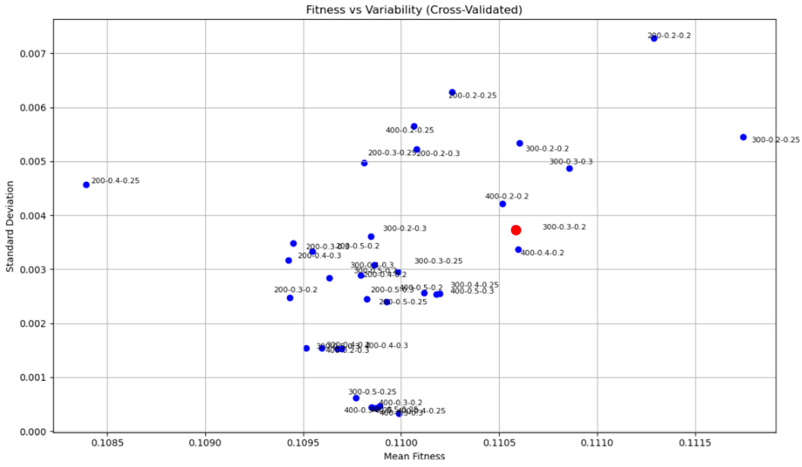
3.4.1. Descriptive Analysis of Parameter Combinations: Mean and Variability of Fitness

To provide a baseline assessment of the parameter space, we performed 50 repeated runs for each of the 36 combinations of population size, mutation rate, and crossover rate. In each run, the artifact distribution and land price grid were held constant to isolate the effects of the algorithmic parameters. For each combination, the mean and standard deviation of the best fitness values were calculated.
The results are visualized in Figure 11 as a scatter plot, with the x-axis representing the average fitness and the y-axis representing standard deviation. This plot helps identify parameter settings that balance both high performance and stability. Rather than using confidence intervals—which assume normality and independence—we report standard deviations as a more transparent indicator of outcome variability under randomized but fixed simulation conditions.
Table 1 provides the underlying numerical values for each of the 36 parameter configurations, listing the mean and standard deviation of the best fitness values obtained over 50 independent runs. Together, Table 1 offer complementary views of performance stability across the explored parameter space.
This approach provides a quantifiable measure of uncertainty without introducing confidence intervals, which may be misleading given the randomized nature of artifact placement in each simulation. By fixing spatial conditions during this phase of parameter tuning, we isolate algorithmic sensitivity from environmental noise.

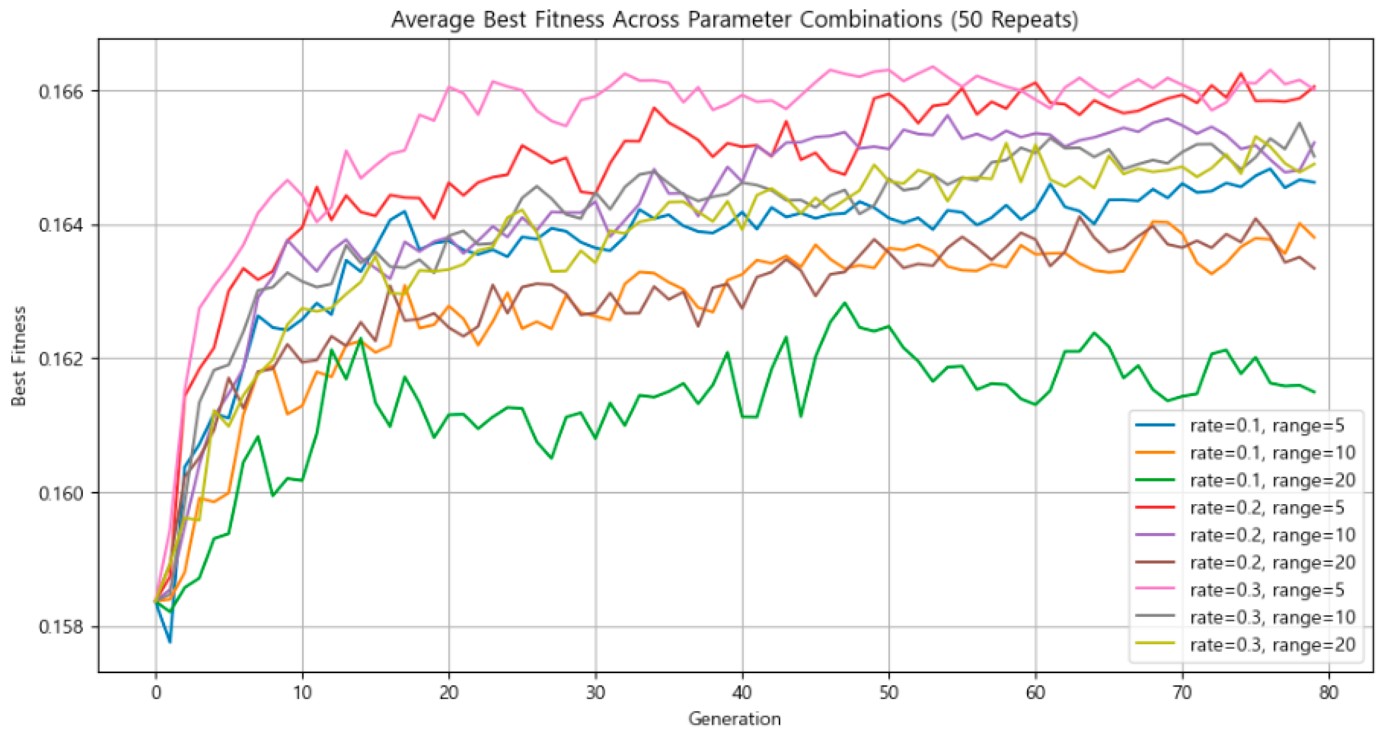
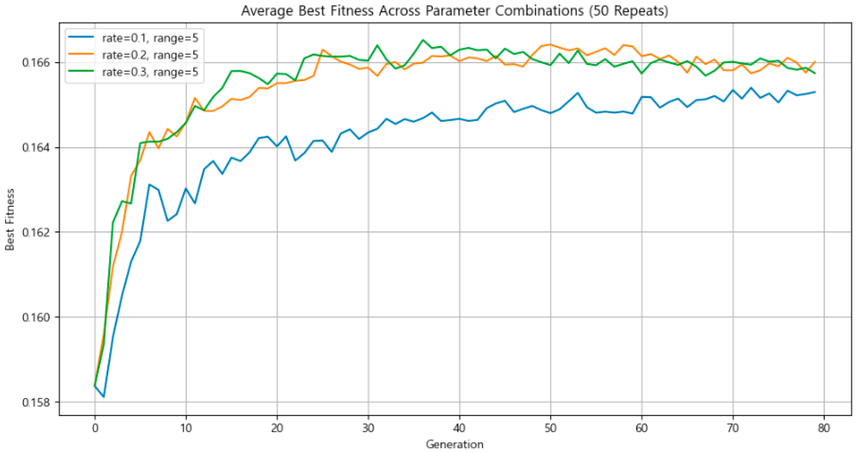
3.4.2. Mutation Intensity and Mutation Rate

To determine appropriate values for the mutation rate and mutation intensity, the number of artifacts was fixed and the population size was set to 300. Simulations were run under various conditions: mutation rates of 10%, 20%, and 30%, and mutation intensity of ±5 km, ±10 km, and ±20 km. Each condition was repeated 50 times, and for each run, the fitness value of the best-performing individual was recorded. (A crossover rate was fixed at 0.3.) The average of these fitness values was then compared across all conditions.
Figure 12 shows the results for the average fitness of the best-performing individuals at each mutation intensity. Across all experimental conditions, a mutation intensity of ±5 km consistently yielded the highest average fitness.
As seen in Figure 12, the optimal mutation intensity for solution quality was ±5 km. Therefore, with the population size fixed at 300 and the mutation intensity set to ±5 km, a second round of experiments was conducted by varying only the mutation rate: 10%, 20%, and 30%.
Based on overall trends, a mutation rate of 20% and 30% appeared to offer a reasonable balance of stability and solution quality. Accordingly, the mutation rate was set to 0.2 for the main simulation (see Figure 13).

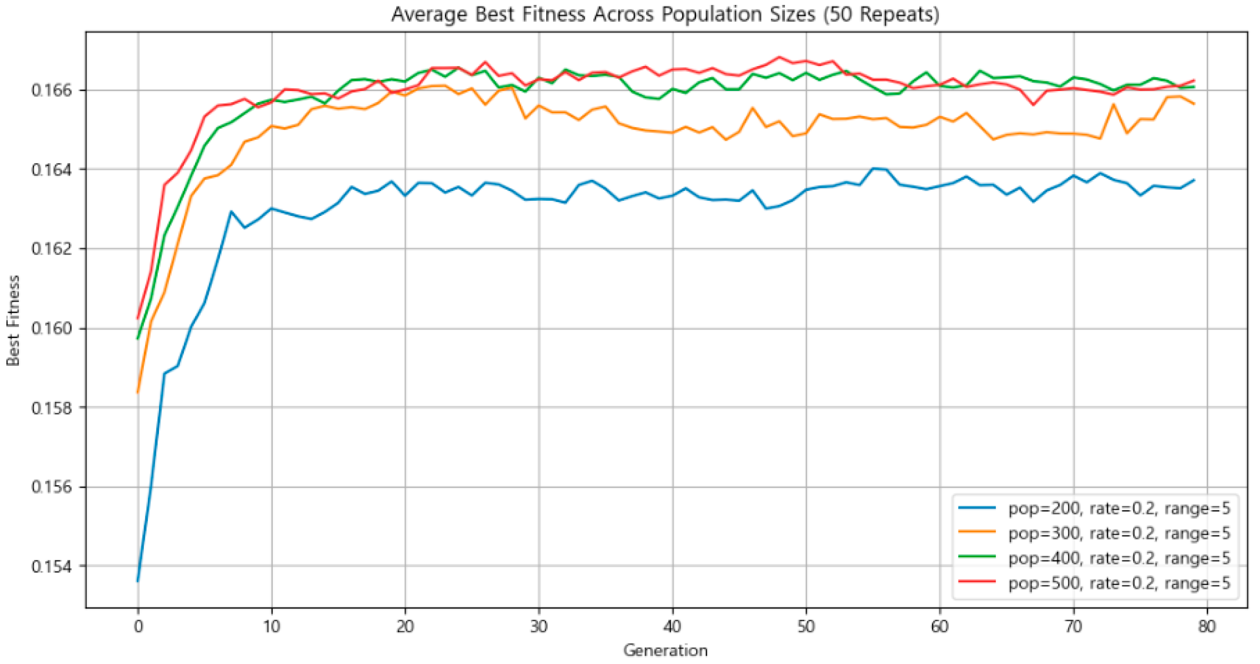
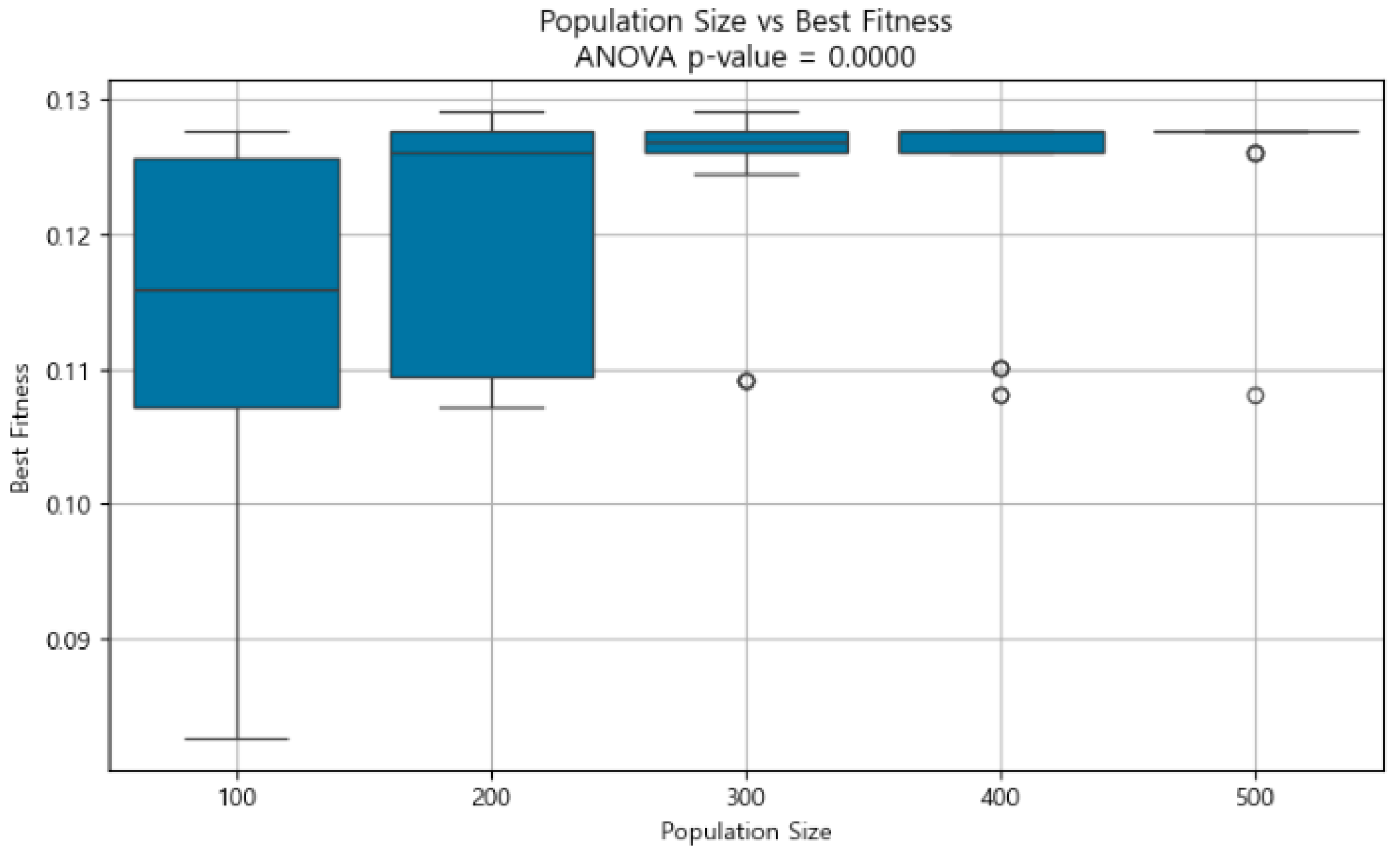
3.4.3. Population Size

As previously stated, the main simulation used a population size of 300. To assess the impact of this parameter, the artifact positions were fixed, the mutation rate was set to 0.2, and the mutation intensity was set to ±5 km. Simulations were run using population sizes of 200, 300, 400, and 500. Each configuration was repeated 50 times, and the average fitness of the best-performing individual was calculated for comparison.
As shown in Figure 14, a population size of 500 produced the highest average fitness overall. However, the greatest improvement in solution quality occurred between population sizes 200 and 300. Moreover, the average fitness values for populations of 400 and 500 were not significantly higher than that of 300. Taking computational resource efficiency into account, a population size of 300 was selected.
As these results indicate, a larger population does not automatically yield better outcomes. While a larger population may explore the search space more thoroughly, it can also introduce disadvantages—such as increased time for advantageous genes to propagate and the persistence of suboptimal individuals. Furthermore, the law of diminishing returns applies: beyond a certain point, the computational cost of increasing the population outweighs the marginal improvement in solution quality. In such cases, reaching the optimal solution requires more generations and higher consumption of computational resources2.

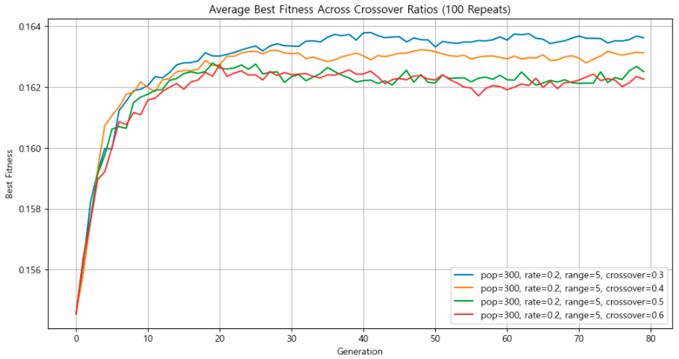
3.4.4. Crossover Rate

To tune the crossover rate, the population size was fixed at 300, mutation rate at 20%, and mutation intensity at ±5 km. Simulations were repeated 100 times for each of the following crossover rates: 0.3, 0.4, 0.5, and 0.6. The fitness values of the best-performing individuals were recorded and averaged for each setting.
As seen in Figure 15, there was a small difference in the fitness of the best-performing individuals across different crossover rates. Based on these findings, the crossover rate was set to 0.3.
Through this series of parameter tuning experiments, it was confirmed that the selected parameter combination in this study achieved a balance between stability and efficiency in the site optimization task.

3.5. Statistical Evaluation of Parameter Tuning: Robustness and Sensitivity Analyses

To complement the earlier visual and descriptive evaluation of parameter tuning, this section provides a more formal statistical assessment of how key GA parameters influence optimization performance. Two approaches were employed: (1) one-way ANOVA tests for individual factors (population size, mutation rate, crossover rate); and (2) two-way ANOVA to evaluate interaction effects. These analyses help to isolate algorithmic sensitivity from environmental randomness and assess the robustness of the optimization framework.

3.5.1. One-Way ANOVA: Single-Factor Sensitivity Analysis

To ensure the reproducibility of results, we fixed the spatial distribution of artifacts and land costs by setting the random seed (np.random.seed(42)). The distribution of individuals is still random (Generation = 50). Under this controlled environment, we conducted one-way ANOVA tests to evaluate the sensitivity of GA performance to each of the three key tuning parameters: population size, mutation rate, and crossover rate.
For the analysis of population size, we held the mutation rate at 0.2 and the crossover rate at 0.3. The results indicate a statistically significant effect on fitness outcomes (F = 9.923, p < 0.001). As summarized, larger population sizes consistently yielded higher average fitness and lower variability.
(1) Size 100: Lower mean fitness and high variance, indicating high diversity but unstable performance.
(2) Size 200: Moderate improvement in mean fitness, though variance remains relatively high.
(3) Size 300–400: Substantial increase in mean fitness with very low variance, reflecting robust convergence and stable outcomes.
(4) Size 500: Highest average fitness and minimal variance, suggesting strong convergence and optimal stability.
As illustrated in Figure 16, the boxplot clearly shows that increasing the population size results in both improved mean fitness and reduced variability. Notably, performance stabilizes markedly at sizes above 300.
These findings align with the general understanding that larger population sizes provide greater search depth and lead to more reliable optimization in the GA. Importantly, the results also suggest that even in relatively simple fitness landscapes with few local optima, a sufficiently diverse initial population plays a crucial role. While the best performance was observed at size 500, the marginal gain beyond 300 was modest compared to the significant increase in computational cost. Thus, a population size of 300 may represent an efficient balance between performance and efficiency.
For the mutation rate analysis, we fixed the population size at 300 and the crossover rate at 0.3. The p-value obtained was 0.4005, indicating no statistically significant difference across the tested levels (0.1, 0.2, 0.3). Similarly, the crossover rate analysis (with the mutation rate fixed at 0.2 and population size at 300) yielded a p-value of 0.4013, again showing no significant variation in performance across levels (0.3, 0.4, 0.5).
Figure 17 further supports the statistical analysis of the mutation and crossover rates, showing minimal differences across parameter levels. The lack of significant variation in these plots is consistent with the high p-values obtained from the ANOVA tests, underscoring the robustness of the GA to these two parameters within the examined range.
These results suggest that within the examined ranges, population size is the primary driver of GA performance sensitivity, whereas mutation rate and crossover rate exhibit robustness, having minimal impact on outcome variability.

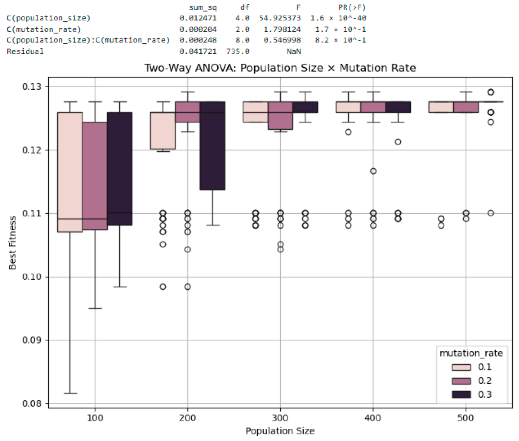
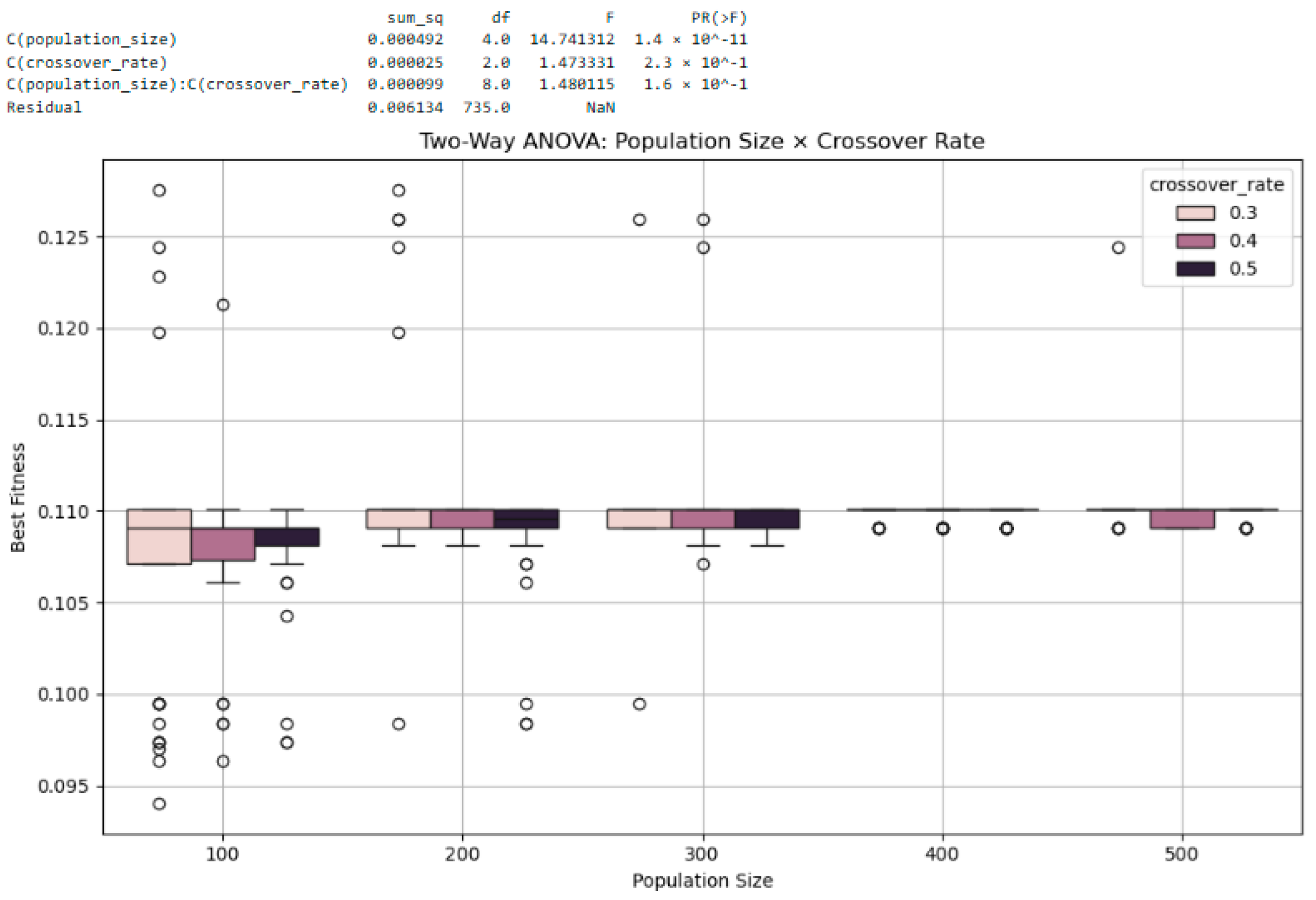
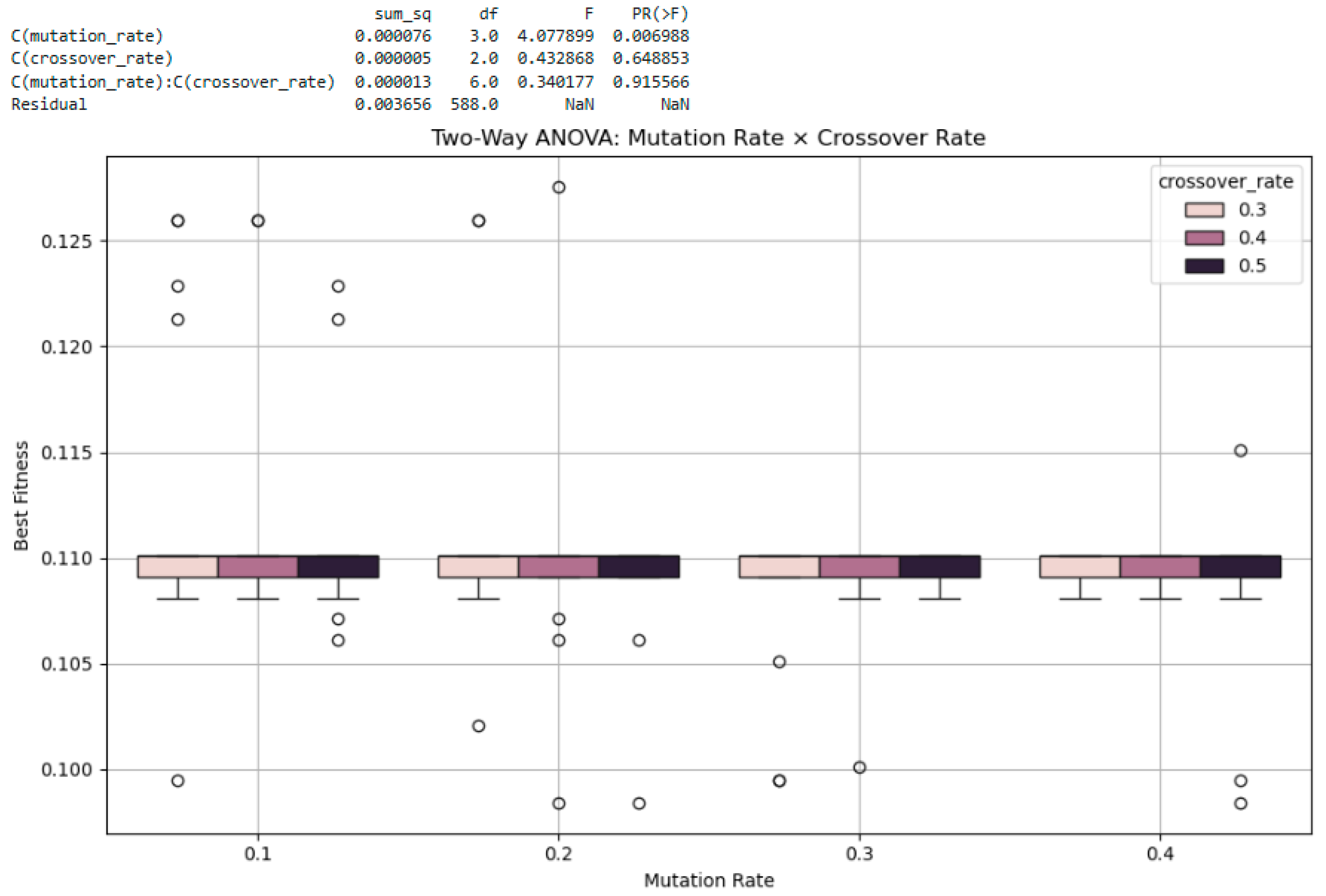
3.5.2. Two-Way ANOVA: Interaction Effects and Multi-Factor Sensitivity

In addition to single-variable analyses, we performed multi-factor statistical tests using two-way ANOVA to explore both main and interaction effects among key parameters. To ensure reproducibility, we fixed artifact distributions and land cost distribution using np.random.seed(42). The initial distribution of individuals is still random. Each parameter pair was evaluated under 50 repeated trials while holding the third parameter constant.
(1) Population Size × Mutation Rate: The mutation rate was varied at three levels (0.1, 0.2, and 0.3), while the crossover rate was fixed at 0.3 (Generation = 50). As shown in Figure 18, population size exhibited a strong main effect on best fitness (F = 54.92, p < 0.001), while the mutation rate had no significant effect (p = 0.166). No interaction was found between the two factors (p = 0.821).
The boxplot illustrates that larger populations consistently achieved better performance and stability, whereas differences between mutation levels were minimal and visually indistinct. When the population size is 300 and the mutation rate is 0.2, the variance appears to be somewhat large. However, this outcome was anticipated to some extent in Section 3.4.1, as this combination was chosen for its strength in solution improvement despite the relatively high variance.
(2) Population Size × Crossover Rate: With the mutation rate fixed at 0.2, population size (100, 200, 300, 400, 500) and crossover rate (0.3, 0.4, 0.5) were tested (Generation = 50). The results (Figure 19) again indicate that population size significantly affects fitness (F = 14.74, p = 1.365299 × 10⁻¹¹), while the crossover rate has no significant effect (p = 0.4354). No interaction effect was observed (p = 0.2089). As population size increases, the boxplot reveals upward shifts in fitness distribution, but crossover variations produce negligible differences.
(3) Mutation Rate × Crossover Rate: A two-way ANOVA was conducted to examine the combined effects of the mutation rate and crossover rate on best fitness, with the population size fixed at 300 (generation = 50). As shown in Figure 20, the analysis revealed a statistically significant main effect for the mutation rate (F = 4.08, p = 0.00699), indicating that mutation rate had an influence on optimization performance. In contrast, the crossover rate did not exhibit a significant main effect (F = 0.43, p = 0.649), and the interaction between mutation rate and crossover rate was also non-significant (F = 0.34, p = 0.916), suggesting that the two parameters did not interact in a meaningful way. The absence of an interaction effect suggests that the two parameters can be tuned independently without considering joint optimization. Interestingly, while the mutation rate showed a statistically significant effect in the previous two-way ANOVA conducted with the crossover rate, it did not have a significant effect when tested in combination with population size (p = 0.179). This suggests that the impact of the mutation rate may diminish as population size increases, likely due to the inherent diversity provided by larger populations. These results indicate that the effectiveness of mutation tuning may be context-dependent, particularly on the chosen population configuration.
The boxplots in Figure 20 visually support this conclusion: the mutation rate shows noticeable shifts in best fitness distributions across levels, while the crossover rate does not introduce meaningful variation. Although some outliers are present, the overall patterns demonstrate that the mutation rate is the more influential parameter in this setting, with the crossover rate playing a comparatively minor role.
In summary, GA performance was highly sensitive to population size, which consistently exhibited a strong and statistically significant effect across all tested combinations (p < 0.001). The mutation rate also showed a significant effect when tested jointly with the crossover rate (p = 0.007), indicating that performance is moderately sensitive to the mutation rate within the examined range. In contrast, the crossover rate demonstrated a robust effect, showing no significant influence on best fitness under any condition tested. Moreover, the absence of significant interaction effects in all three ANOVA analyses suggests that the parameters can be tuned independently, without requiring complex combinatorial calibration. This independence allows for simplified and modular parameter optimization in practical implementations.

4. Discussion

4.1. Feasibility and Performance of Economic Site Optimization

The simulation results provide clear answers to the first and second research questions. Using the optimal parameter combination—population size of 300, mutation rate of 0.2, mutation intensity of ±5 km, and crossover rate of 0.3—the GA successfully identified and preserved economically efficient sites for drone station installation within the virtual region.
As shown in Figure 1, the best fitness stabilized at 0.1649 from Generation 25 onward, with a slight increase to 0.1684 by Generation 75. The average fitness peaked at 0.1341, confirming that not only were elite individuals preserved, but the population as a whole became increasingly efficient. The persistent gap between the best and worst individuals reaffirmed the algorithm’s ability to systematically filter out underperforming candidates over time.
Sequential visualizations (Figure 2, Figure 3, Figure 4, Figure 5, Figure 6 and Figure 7) further reinforce this trend. In Generation 0 (Figure 2), individuals were randomly distributed with no clustering. Nevertheless, a single high-fitness candidate emerged early, highlighting the algorithm’s capacity to identify favorable areas even in unstructured settings. By Generation 10 (Figure 3), population clustering around high-potential zones began, with average fitness tripling from its initial level. Coverage circles started aligning with artifact-rich areas, signaling the onset of spatially guided optimization.
A pivotal phase emerged between Generations 25 and 30 (Figure 4 and Figure 5), where overlapping density increased significantly—37 and then 41 individuals converged at the same coordinates. This convergence was not merely positional but structural, as distinct lineages independently arrived at the same solution. Visual patterns showed increasingly efficient artifact coverage and clearer alignment between coverage areas and favorable cost zones.
By Generation 40 (Figure 6), convergence was effectively complete, with 45 individuals overlapping at the optimal location. Despite continued mutation, this structure remained stable through Generation 75 (Figure 7). The best-performing candidate persisted, and the population remained densely clustered around the same coordinate, showing no emergence of better alternatives. This durability of the solution, despite ongoing stochastic variation, suggests robustness in both convergence and outcome.
Importantly, this convergence emerged not through dominance of a single lineage but through collective reinforcement—multiple individuals repeatedly locating the same site under evolutionary pressure. This pattern implies a high degree of repeatability, an essential trait for real-world infrastructure planning.
Altogether, these findings validate the feasibility of a GA for economic site optimization. The algorithm balanced artifact coverage with land cost, achieved stable convergence, and displayed resilience to mutation. The structured emergence of the final solution—supported by spatial and fitness-based evidence—confirms the potential of a GA as a dependable decision-support tool for planning drone stations in cultural heritage protection.

4.2. Contributions of Visualization to Economic Site Optimization

This study not only presents numerical outputs from GA-based site optimization but also provides a structured visualization framework for interpreting the internal logic and trajectory of the optimization process. The visualizations in Figure 2, Figure 3, Figure 4, Figure 5, Figure 6 and Figure 7 offer more than illustrative support—they function as analytical tools that enhance understanding, repeatability, and potential policy applicability.
First, the visual progression across generations clearly shows how the GA transitions from a phase of broad exploration to a phase of structured convergence. In Generation 0 (Figure 2), individuals are uniformly scattered, coverage areas overlap heavily, and there is no spatial order. However, as early as Generation 10 (Figure 3), one observes the emergence of clusters, with coverage areas beginning to align around promising zones—visually corresponding to the increase in average fitness.
From Generations 25 through 40 (Figure 4, Figure 5 and Figure 6), the visualizations reveal a concentrated migration of individuals toward a specific site. The density of overlapping markers—especially in Generation 40, where over 50 individuals share the same coordinate—visually demonstrates that the algorithm has not merely “settled” but structurally converged on an optimal location. Importantly, these patterns are not driven by a single outlier but by multiple lineages independently arriving at the same solution. This type of visual convergence provides intuitive confirmation of the optimization’s robustness—something that raw fitness values alone cannot fully convey.
Second, the clarity and simplicity of the final visual state (Figure 7, Generation 75) help confirm that the GA’s behavior is not erratic or overly sensitive to mutation. Despite ongoing mutation and recombination operations, the convergence remains intact. Even coverage patterns (green and black dashed circles) become cleaner and less redundant over time, signaling increased spatial efficiency in how the algorithm distributes candidate solutions. These patterns support the claim that the optimization has reached a globally stable solution and has maintained diversity in non-critical regions without destabilizing the optimal cluster.
Third, from a broader methodological perspective, these visualizations significantly improve the interpretability and communicability of simulation-based optimization. In contexts such as cultural heritage protection—where public consensus, administrative decision-making, and spatial equity are essential—the ability to explain how and why a certain location was selected is as important as the numerical justification. Through visual evidence of convergence, robustness, and spatial logic, this study contributes to the development of transparent and explainable algorithmic decisions in infrastructure planning.
Furthermore, these visuals help demonstrate that optimization is not a “black box” process but a replicable and intelligible system of adaptive learning. This enhances the credibility of algorithmic approaches in domains where stakeholder understanding is crucial. When paired with statistical validation, visualizations like those shown in this study can bridge the gap between technical rigor and real-world policy needs.
That said, it is important to emphasize the modeling character of these visualizations. The maps presented do not represent real-world topography, regulatory constraints, or detailed land-use zoning. Instead, they are abstract representations within a simplified virtual space. As problem complexity increases, visualization itself becomes more challenging and must be carefully designed to avoid misrepresentation. Thus, while visualization supports interpretability, it should always be read in context—serving not as a literal map but as a conceptual lens through which optimization logic can be understood.

4.3. Interpreting the Results of Parameter Tuning

The central research question of this study was whether a GA could effectively identify economically optimal locations for drone stations dedicated to cultural heritage protection and research. In addressing this question, parameter configuration played a decisive role. The tuning results presented in Section 4 demonstrated that parameter settings were not merely about computational efficiency—they provided the structural foundation necessary for reaching a global optimum.
For example, a population size of 300 increased the likelihood of placing at least one initial individual near the global optimum within the 100-grid search space, thus facilitating faster and more stable convergence. In combination with a mutation rate of 0.2 and mutation intensity of ±5 km, the GA preserved exploration while maintaining convergence stability. The crossover rate of 0.3 contributed to maintaining fit individuals while also ensuring the sufficient generation of new candidates.
These settings were supported by the simulation results: from Generation 40 onward, the best-performing individual consistently reappeared, and overlapping of individuals in the optimal grid cell increased. This can be interpreted as evidence that the chosen parameter set enhanced the algorithm’s stability and repeatability. Even when a high-performing individual was altered through mutation, others overlapping at the same site preserved the optimal solution.
The eight-fold difference between the best and worst fitness values suggests that the configured GA was not simply identifying a valid solution but functioning as a tool to explore complex trade-offs between cost and efficiency. The early rise in average fitness followed by stable convergence implies that while premature convergence was avoided, solution quality continued to improve.
Taken together, these findings suggest that, under appropriate parameter settings, a GA can be a reliable tool for economically optimizing drone station placement in the context of cultural heritage preservation and research.

4.4. Enhancing the Realism of the Model

While the proposed GA-based optimization model demonstrated consistent performance under controlled simulation settings, questions may arise regarding its external validity—particularly in relation to the spatial and economic heterogeneity observed in real-world cultural heritage contexts. To address this, we designed additional robustness experiments to examine how varying artifact distributions and land price patterns influence optimization outcomes. The following subsections present the results of these extended tests.

4.4.1. Artifact Density and Spatial Distribution

To evaluate the sensitivity of optimization outcomes to spatial and economic heterogeneity, we conducted a full factorial experiment by systematically varying both the spatial distribution of artifacts and the distribution of land prices. Artifact distributions were defined as follows: a uniform setting with artifacts randomly scattered across the 50 × 50 km region; a clustered setting generated using Gaussian blobs centered at five locations; and a mixed setting combining half uniform and half clustered placements. Land price patterns were also varied: the uniform mode assigned random values between 500 and 5000 to each grid cell; the skewed mode followed a clipped normal distribution centered around 3000; and the clustered mode embedded a high-price zone within an otherwise low-cost grid. Each of the resulting 3 × 3 = 9 combinations was simulated 100 times, totaling 900 independent trials. The simulation space consisted of a 10×10 grid of candidate station locations and 200 artifacts. Fitness was calculated as the number of artifacts within 20 km of a proposed station location divided by the land cost at that location.
The results were analyzed using two-way ANOVA, which confirmed that both artifact distribution (F = 53.32, p < 0.001) and land price pattern (F = 138.84, p < 0.001) significantly influenced the best fitness scores. The detailed results are presented in Table 2, which shows that both main effects were statistically significant (all p < 0.001), indicating that optimization outcomes are sensitive to spatial and economic structural conditions. Moreover, the interaction between the two factors was not statistically significant (F = 1.36, p = 0.248), suggesting that optimization outcomes are not shaped by complex spatial–economic interdependencies, but are merely additive.
As visualized in Figure 21, average fitness varied substantially across conditions. The most favorable results occurred when artifacts were clustered and land prices were also clustered (mean fitness = 0.2309), while the least favorable configuration involved uniform artifacts and skewed prices (mean fitness = 0.1313). These patterns reveal that dense cultural regions paired with affordable land tend to yield better optimization outcomes, while spatial fragmentation and economic inequality tend to suppress performance.
These findings affirm that while the GA model is robust across various parameter settings, its performance is indeed sensitive to the underlying structural assumptions about the spatial and economic landscape. This sensitivity underscores the importance of incorporating realistic distribution patterns when applying such optimization models to real-world cultural heritage planning.

4.4.2. Integration of Elevation-Based Construction Cost and Distance-Based Access Cost and Cost Model Sensitivity Analysis

To overcome the limitations of using land price alone in the original cost model, we expanded the optimization framework by incorporating two additional spatially variable cost components: construction cost, linked to elevation, and access cost, based on proximity to a central reference point. These three cost layers were linearly combined to define total site cost, which was then integrated into the fitness function of the GA as the denominator in a coverage/cost ratio. The modified fitness was computed as the number of cultural artifacts within a 20 km radius divided by the sum of land price, construction cost, and access cost at each candidate site.
Simulations were performed over 1000 independently seeded trials, each using a 50 × 50 km region subdivided into a 10 × 10 grid of candidate sites. Reproducibility was ensured by fixing the random seed per trial (np.random.seed(trial)), while each scenario featured a newly randomized placement of 200 artifacts.
-
Land prices were randomly drawn from a uniform distribution between KRW 5,000,000 and KRW 50,000,000.
-
Construction cost was computed by applying a multiplier (ranging from 1.0 to 1.8) to a fixed base cost of KRW 10,000,000, proportionally increasing with elevation (from 0 to 800 m in 100 m steps).
-
Access cost was modeled as KRW 100,000 per kilometer of Euclidean distance from the region’s geometric center (i.e., the point (25 km, 25 km)), representing a hypothetical urban core.
Based on one-way ANOVA, all three cost components—land price, construction cost, and access cost—exhibited statistically significant effects on optimization outcomes (p < 0.001). Land price showed the strongest effect (F = 88,982.45), followed by construction cost (F = 22,147.31) and access cost (F = 3050.92). Regression analysis using standardized inputs further confirmed that land price had the strongest negative effect on fitness (β = −0.72), followed by construction cost (β = −0.38) and access cost (β = −0.30), with a high overall explanatory power (R2 = 0.79). Summary statistics also highlighted the disproportionately high standard deviation of land prices (KRW 6.72 million) compared to the other cost factors, emphasizing the larger scale and variance of land prices as a key driver of their dominant impact on optimization performance.
These findings enhance the model’s practical relevance, demonstrating that location-based cost considerations—especially land acquisition costs—can significantly influence optimal siting outcomes. The extended model remains computationally lightweight while improving its alignment with real-world constraints. Future extensions may integrate empirically derived elevation maps, transportation networks, or multi-nodal urban hierarchies for greater realism.

4.4.3. Scaling up the Problem: Effects on GA and GA + HC Performance

To further assess the model’s practical scalability, we conducted additional experiments under a substantially enlarged problem setting—expanding the simulated area to 200 × 200 km2, increasing the number of artifacts to 1000, and optimizing for three drone stations instead of one. While the problem scale was increased, the GA’s population size and generation count were deliberately kept modest (pop_size = 360 or 400, generations = 100) to simulate a constrained search scenario. This design allowed us to evaluate whether augmenting GA with a local search operator (hill climbing) could compensate for limited global search capacity under such expanded conditions.
The step size of the hill climbing algorithm was set to 2 km, with a maximum of 100 iterations. To ensure equivalent computational cost for performance comparison, the standalone GA model was configured with a population size of 400, while the GA + HC hybrid model used a population size of 360. All other GA parameters were kept identical across both models.
To ensure both reproducibility and scenario diversity, each trial was initialized with a distinct random seed by invoking np.random.seed(trial) and random.seed(trial). This approach enabled the generation of 300 independent spatial configurations, each with a unique distribution of artifacts, while guaranteeing that the entire experiment could be fully replicated. By combining controlled randomness with repeated simulations, the study maintains both internal consistency and robustness to spatial variability.
Over 300 trials, the GA + Hill Climbing (GA + HC) model consistently exhibited slightly higher performance than the standalone GA. The mean best fitness increased from 0.0611 (GA) to 0.0622 (GA + HC), and this difference reached statistical significance (t(598) = −1.99, p = 0.047), suggesting that the integration of hill climbing yielded a measurable improvement in solution quality. However, the difference in mean overall fitness was more modest—0.0454 (GA) vs. 0.0459 (GA + HC)—and did not reach statistical significance (t(598) = −1.12, p = 0.261), indicating that the overall population-level performance remained largely comparable.
These gains were achieved with only a modest increase in computational cost: the average number of fitness function evaluations rose from 40,400 (GA) to 41,410 (GA + HC), representing an increase of roughly 2.5%. The total runtime for all 300 paired trials was 2337.16, confirming that the added local search component remained computationally feasible.
Taken together, these results support the effectiveness of hybridizing GA with hill climbing, especially in contexts where even marginal gains in best fitness are meaningful or when the refinement of elite solutions is critical. While the improvement in overall population fitness was not statistically significant, the observed enhancement in peak performance—achieved with only a modest increase in computational cost—demonstrates the practical value of incorporating local search.
Moreover, these findings suggest that hybrid GA models can offer a scalable and computationally manageable approach for larger spatial optimization problems, particularly in scenarios where extensive parameter tuning is constrained by limited resources. Further exploration of local search configurations (e.g., step size, iteration limits) may yield additional improvements in solution quality and convergence efficiency.

5. Conclusions

5.1. Summary of Findings and Contributions

This study began with the recognition that drones can play a critical role in the research and preservation of cultural heritage sites. It proposed a method for identifying and visualizing the economically optimal locations for medium-to-large-scale drone stations intended for cultural heritage protection and research, using a GA. While prior studies have largely focused on the technological feasibility of drones for heritage monitoring, little attention has been paid to the optimization of drone station placement from an economic perspective.
To address this gap, the present study conducted GA-based optimization experiments within a 2500 km2 virtual environment, avoiding reliance on any specific real-world case. Through repeated simulations, optimal GA parameters were identified by systematically tuning key values—population size, mutation rate, mutation intensity, and crossover rate. The resulting optimal configuration was a population size of 300, mutation rate of 0.2, mutation intensity of ±5 km, and crossover rate of 0.3. This combination was found to strike the most effective balance between exploration and convergence.
Under these conditions, the simulation showed that candidate drone station locations gradually converged toward regions with lower land prices that also enabled coverage of a greater number of artifacts. No premature convergence was observed, and the fitness of the best-performing individual stabilized between Generations 40 and 75. The visualization results clearly illustrated not only the trajectories of the best individuals but also the broader population’s movement toward economically efficient zones—where many artifacts could be monitored at relatively low cost. This visual evidence supported the interpretability of the optimization process and showed how a GA can function as a decision support tool by making complex algorithmic reasoning more accessible to policymakers.
Thus, the study demonstrates the potential of a GA as both a powerful search algorithm and a visualizable framework for economically optimizing drone station placement for cultural heritage protection and research. Despite being based on a simplified simulation model, this research shows that a GA can be a useful tool in addressing this type of problem. Moreover, the proposed approach is not confined to a particular case, suggesting broader applicability to various regions and conditions.

5.2. Limitations and Future Research Directions

While the present study provides a foundational framework for GA-based optimization of drone station siting, several important limitations remain—many of which point to future research directions.
(1) Lack of data-driven model calibration and implementation pathways: The current study relies entirely on a simplified virtual environment. Future research could enhance realism by integrating real-world geographic and administrative data through spatial multi-criteria decision frameworks. For instance, Bi et al. [23] proposed a GIS–FAHP–MABAC model to identify optimal locations for electric vehicle charging stations using real-world slope, land-use, population, and transportation data. Building on this methodology, GA-based optimization could be extended to incorporate actual coordinates of heritage sites, elevation maps, land value registers, and disaster risk indices. Model calibration could also be pursued by validating simulation outputs against expert-defined priority zones. This would enable a smoother transition from simulation to implementation.
(2) Single-objective optimization framework: The study currently adopts a single-objective framework that maximizes artifact coverage per unit of land cost. However, real-world planning decisions often involve complex trade-offs among multiple, sometimes conflicting, goals. For example, maximizing coverage may come at the expense of increased construction or operational costs, or may conflict with accessibility requirements for remote areas. Future studies could adopt a Multi-Objective Genetic Algorithm (MOGA) approach to optimize multiple criteria—such as cost, coverage, accessibility, and long-term maintainability—without requiring fixed weightings.
(3) Assumption of idealized circular drone coverage: One notable limitation lies in the assumption of idealized circular coverage with a fixed 20 km radius. In practice, environmental constraints such as terrain occlusion, vegetation density, and signal interference may significantly reduce the effective coverage range of unmanned aerial systems (UAS). This simplification may result in optimistic bias, particularly in mountainous or urbanized regions. Incorporating realistic coverage maps derived from terrain and line-of-sight analysis would improve model accuracy.
(4) Need for hybrid models combining GA with MCDM: Although this study focused on simulation-based optimization, future applications could benefit from combining GA with multi-criteria decision-making (MCDM) frameworks. Studies such as Bi et al. [23] have shown how algorithmic optimization can be grounded in spatial data and stakeholder input using integrated GIS–FAHP–MABAC approaches. Hybrid models that fuse GA with MCDM could enhance the interpretability and practical relevance of the optimization, especially when engaging with real-world planning stakeholders.

Supplementary Materials

The following supporting information can be downloaded at: https://www.mdpi.com/article/10.3390/systems13060435/s1.

Author Contributions

Conceptualization, S.K.; formal analysis, S.K.; funding acquisition, Y.N.; methodology, S.K.; supervision, Y.N.; visualization, S.K.; writing—original draft, S.K.; writing—review and editing, S.K. All authors will be updated at each stage of manuscript processing, including submission, revision, and revision reminder, via emails from our system or the assigned Assistant Editor. All authors have read and agreed to the published version of the manuscript.

Funding

This research was supported by the Ministry of Education of the Republic of Korea and the National Research Foundation of Korea (NRF) under grant number NRF-2023S1A5C2A02095114.

Institutional Review Board Statement

Not applicable.

Informed Consent Statement

Not applicable.

Data Availability Statement

The python code presented in this study is available in the Supplementary Materials.

Conflicts of Interest
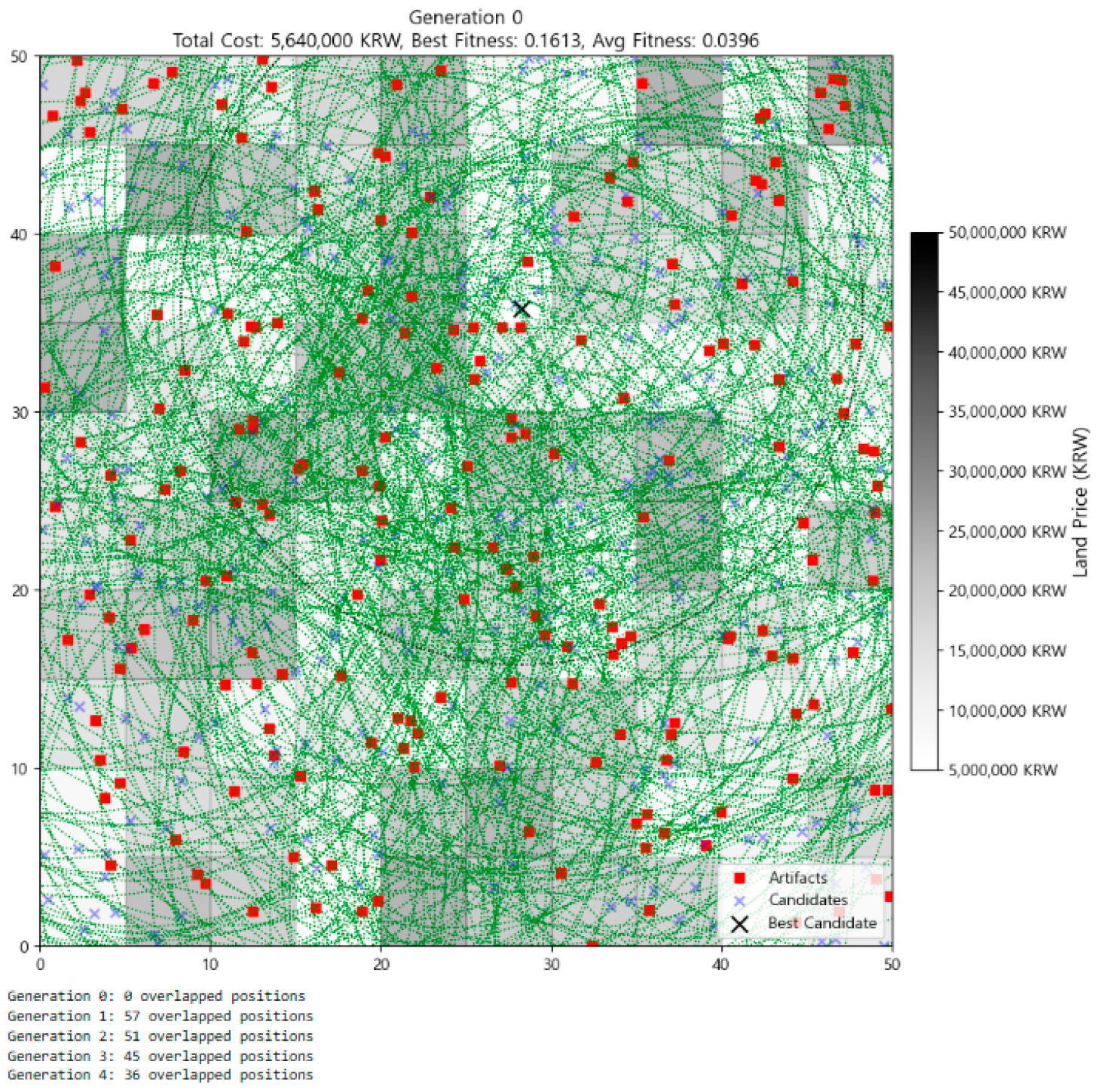
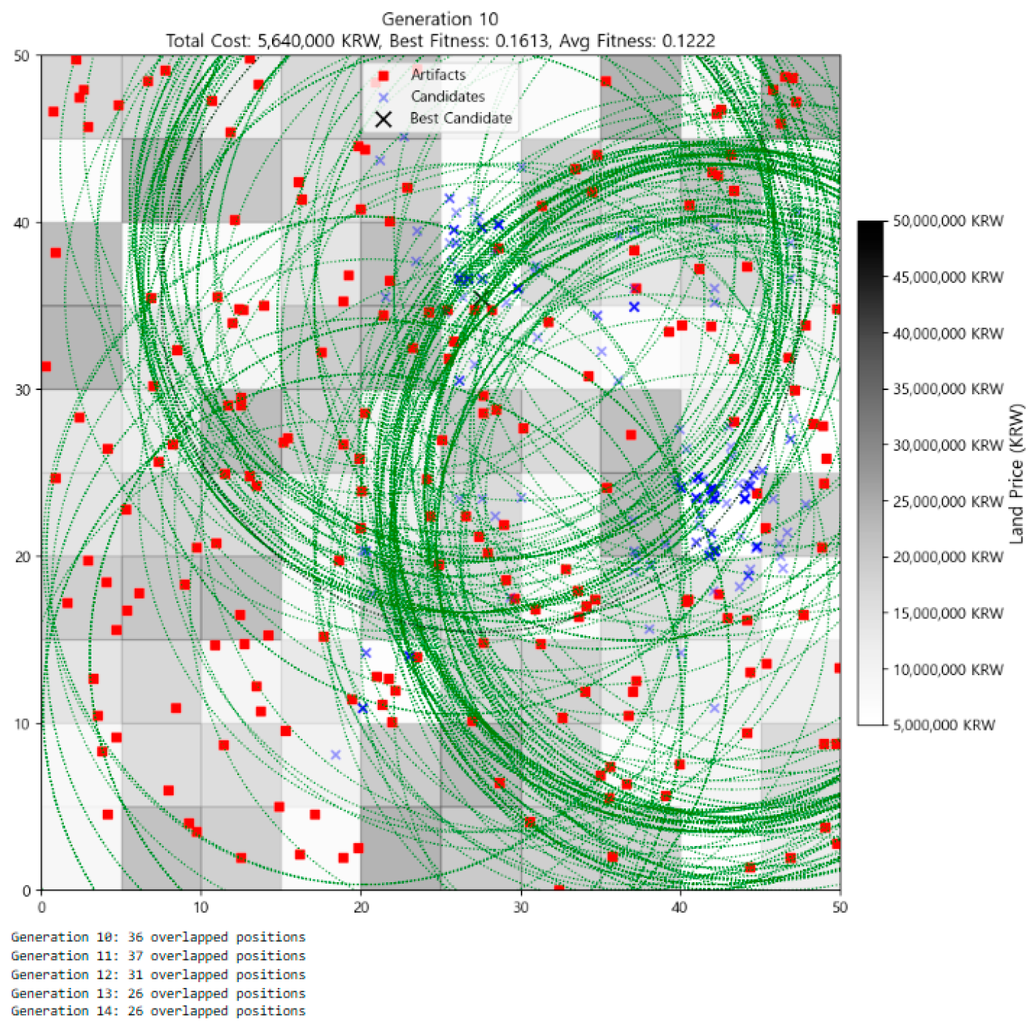
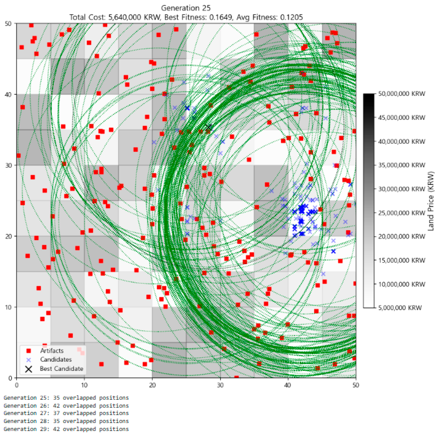
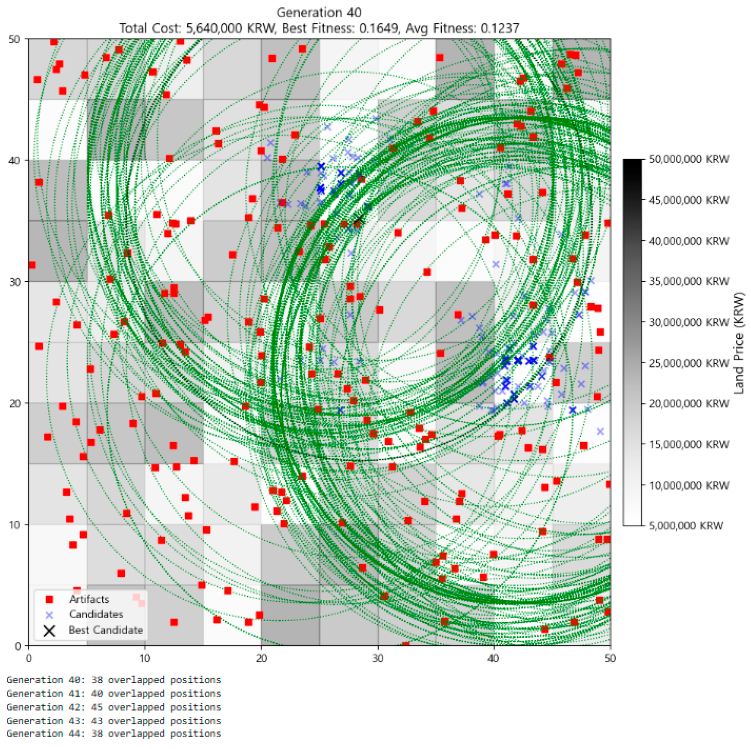
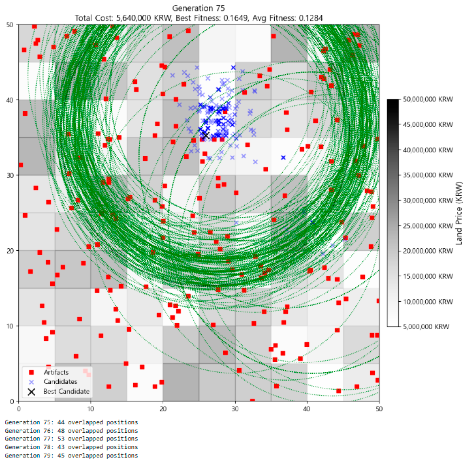
The authors declare no conflicts of interest.

Notes

1
Meanwhile, as generations progress, it may appear that the number of individuals is decreasing. However, this is an illusion caused by individuals increasingly overlapping at the same location. The actual number of individuals remains constant at 300 throughout all generations, a fact that can be confirmed with code output such as print(f“Generation {gen}: {len(individuals)} individuals”).
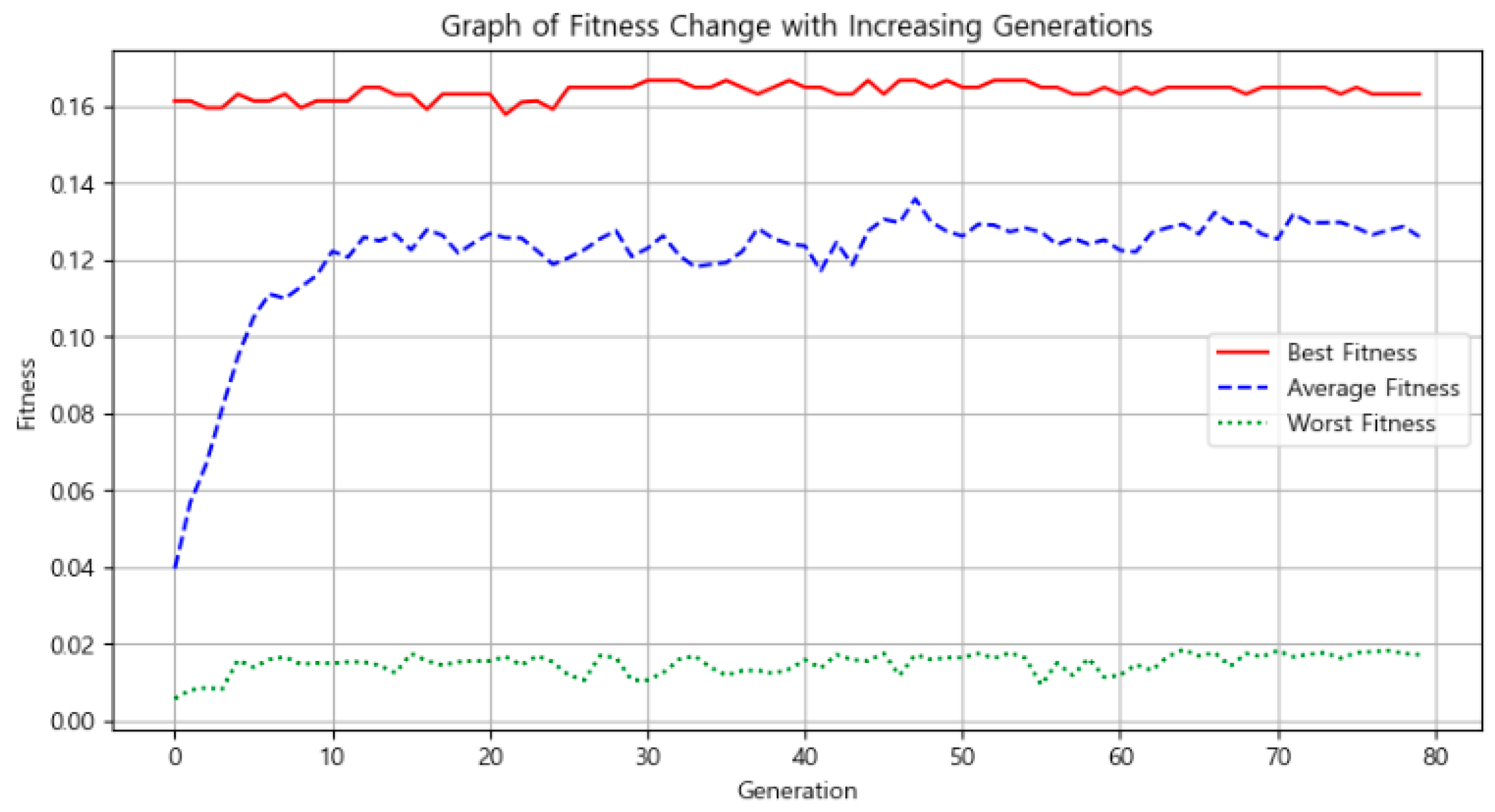
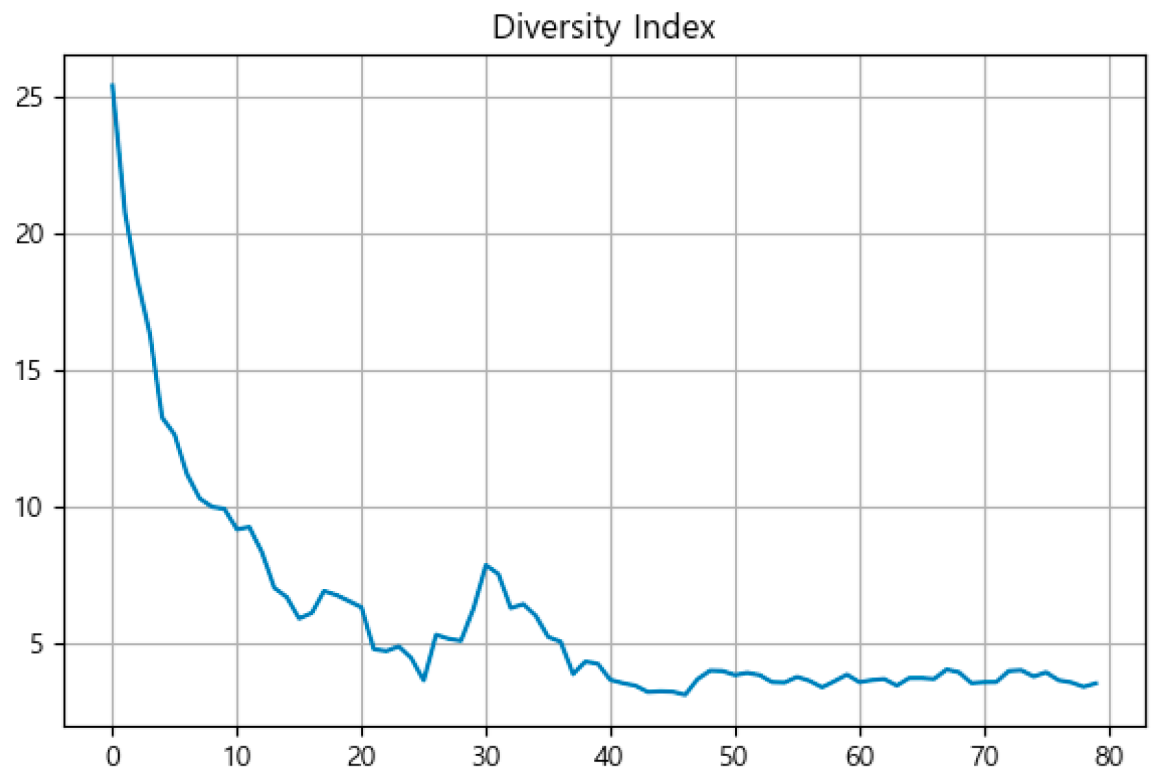
2
The identification of optimal parameter values often depends on how many simulation iterations are required for the GA to reach the optimal solution. The parameter configuration that results in the fewest iterations needed to achieve the optimum is typically regarded as the optimal setting.

References

  1. Lee, T.H.; Kang, J.W.; Ohk, Y.J.; Kim, J.H.; Lee, S.Y. Development of Remote Drone Station System for Water Disaster Management. In Proceedings of the Korean Society of Civil Engineers (KSCE) Convention, Chonnam, Republic of Korea, 18 October 2023. [Google Scholar]
  2. Kim, D.H.; Lee, J.H.; Cheon, W.Y. A Study on Application of Unmanned Aerial Vehicles (UAV) in the Disaster and Safety Field of Cultural Properties. J. Natl. Herit. 2020, 5, 225–232. [Google Scholar]
  3. Ko, M.H.; Kang, S.J. A Study on the Photogrammetric Data Acquisition for the Disaster Prevention of Wooden Architectural Properties with Unmanned Aerial Vehicles (UAV). In Proceedings of the Annual Conference of Architectural Institute of Korea (AIK), Gangwon, Republic of Korea, 25 October 2023. [Google Scholar]
  4. Ko, S.J. Buan County Selected for “Cultural Heritage Drone Station Construction” Project. Available online: https://www.newsis.com/view/?id=NISX20210118_0001309044 (accessed on 18 January 2021).
  5. Heo, U.H.; Lee, W.Y. A study on the utilization of drones and aerial photographs for searching ruins with a focus on topographic analysis. MUNHWAJAE Korean J. Cult. Herit. Stud. 2018, 51, 22–37. [Google Scholar]
  6. Klüver, C.; Klüver, J.; Schmidt, J. Modelling Complex Processes through Nature-Inspired Methods: Soft Computing and Related Techniques, 2nd ed.; Springer: Berlin/Heidelberg, Germany, 2012. [Google Scholar]
  7. Lee, G.S.; Choi, Y.W.; Lee, M.H.; Kim, S.G.; Cho, G.S. Reconnaissance Surveying for Cultural Assets using Unmanned Aerial Vehicle. J. Korean Cadastre Inf. Assoc. 2016, 18, 25–34. [Google Scholar]
  8. DJI Enterprise. Utilizing LiDAR to Discover Ancient Mayan Civilizations. Available online: https://enterprise-insights.dji.com/blog/utilizing-lidar-to-discover-ancient-mayan-civilizations (accessed on 20 March 2025).
  9. Jeon, Y.G.; Lee, M.S.; Kim, Y.R.; Lee, M.H.; Choi, M.J.; Choi, K.H. Utilization of Hyperspectral Image Analysis for Monitoring of Stone Cultural Heritages. J. Conserv. Sci. 2015, 31, 395–402. [Google Scholar]
  10. Ko, H.J.; Yoon, S.J.; Oh, H.; Roh, K.; Kim, E.; Kim, S.; Lim, H.; Choi, S. Planning on R&D for Securing Disaster Response and Enhancing Resilience; National Disaster Management Research Institute: Ulsan, Republic of Korea, 2019. [Google Scholar]
  11. Koza, J.R. Genetic Programming; MIT Press: Cambridge, MA, USA, 1992. [Google Scholar]
  12. Park, J.M.; Choi, Y.J. Utilization of Drone for Strengthening Safety Management of Wooden Cultural Assets: Focused on Fire Prevention. Korean Secur. J. 2021, 67, 217–233. [Google Scholar]
  13. Goldberg, D.E. Genetic Algorithms in Search, Optimization, and Machine Learning; Addison-Wesley: Boston, MA, USA, 1989. [Google Scholar]
  14. Holland, J.H. Adaptation in Natural and Artificial Systems; MIT Press: Cambridge, MA, USA, 1975. [Google Scholar]
  15. Köhler-Bußmeier, M. Koordinierte Selbstorganisation und Selbstorganisierte Koordination: Eine Formale Spezifikation Reflexiver Selbstorganisation in Multiagentensystemen Unter Spezieller Berücksichtigung der Sozialwissenschaftlichen Perspektive. Habilitation Thesis, University of Hamburg, Hamburg, Germany, 2008. [Google Scholar]
  16. Korean Heritage Service Channel. Using Drones for Cultural Heritage Analysis?! Heritage Meets Science. Available online: https://youtu.be/qC0yg0xaDvE (accessed on 15 September 2022).
  17. Kim, M.H. Haman County to Protect Cultural Heritage via Drones. Available online: https://www.knnews.co.kr/news/articleView.php?idxno=1406256 (accessed on 12 June 2023).
  18. Weicker, K. Evolutionäre Algorithmen, 3rd ed.; Springer: Berlin/Heidelberg, Germany, 2015. [Google Scholar]
  19. Stewart, T.; Janssen, R.; van Herwijnen, M. A Genetic Algorithm Approach to Multi-Objective Land Use Planning. Comput. Oper. Res. 2004, 31, 2293–2313. [Google Scholar] [CrossRef]
  20. Jaramillo, J.H.; Bhadury, J.; Batta, R. On the Use of Genetic Algorithms for Location Problems. Comput. Oper. Res. 2002, 29, 761–779. [Google Scholar] [CrossRef]
  21. Xie, Y.; Shaw, W.J.; Wang, W.; Seiple, T.E.; Rishel, J.P.; Rutz, F.C.; Chapman, E.G.; Allwine, J. A Genetic Algorithm Used to Optimize the Siting of Meteorological Monitoring Stations. In Proceedings of the International Conference on Genetic and Evolutionary Methods (GEM’07), Las Vegas, NV, USA, 25–28 June 2007; Arabnia, H.R., Yang, J.Y., Yang, M.Q., Eds.; CSREA Press: Athens, GA, USA, 2007; pp. 81–87. [Google Scholar]
  22. Altiparmak, F.; Gen, M.; Lin, L.; Paksoy, T. A Genetic Algorithm Approach for Multi-Objective Optimization of Supply Chain Networks. Comput. Ind. Eng. 2006, 51, 196–215. [Google Scholar] [CrossRef]
  23. Bi, H.; Gu, Y.; Lu, F.; Mahreen, S. Site Selection of Electric Vehicle Charging Station Expansion Based on GIS-FAHP-MABAC. J. Clean. Prod. 2025, 507, 145557. [Google Scholar] [CrossRef]
  24. Park, I.O.; Kim, W.J. A Study on the Optimal Planning for Dong Office Location by Genetic Algorithm. IE Interfaces 2009, 22, 223–233. [Google Scholar]
  25. Zadeh, L.A. Fuzzy Logic, Neural Networks, and Soft Computing. Commun. ACM 1994, 37, 77–84. [Google Scholar] [CrossRef]
  26. Seising, R.; Sanz, V. Soft Computing in Humanities and Social Sciences; Springer: Berlin/Heidelberg, Germany, 2012; Volume 273. [Google Scholar]
  27. Hwang, H.S. Evolutionary Computation and Evolutionary Design by Computers; Naeha Publishing: Seoul, Republic of Korea, 2002. [Google Scholar]
Figure 1. Graph of fitness change with increasing generations.
Systems 13 00435 g001
Figure 2. Distribution of individuals at Generation 0.
Systems 13 00435 g002
Figure 3. Distribution of individuals at Generation 10.
Systems 13 00435 g003
Figure 4. Distribution of individuals at Generation 25.
Systems 13 00435 g004
Figure 5. Distribution of individuals at Generation 30.
Systems 13 00435 g005
Figure 6. Distribution of individuals at Generation 40.
Systems 13 00435 g006
Figure 7. Distribution of individuals at Generation 75.
Systems 13 00435 g007
Figure 8. Change in Diversity Index across generations.
Systems 13 00435 g008
Figure 9. Shannon Entropy of population distribution per generation.
Systems 13 00435 g009
Figure 10. A boxplot comparing the best fitness values obtained through random placement and Genetic Algorithm across 100 trials. In each trial, a different artifact distribution was randomly generated, but both methods were applied to the same environment. The GA shows a significantly higher and more consistent performance than RP.
Systems 13 00435 g010
Figure 11. Scatter plot of mean fitness versus standard deviation across GA parameter combinations (population size, crossover rate, mutation rate). Each point represents 50 simulation runs under fixed spatial conditions. Lower-left region indicates configurations with both high average performance and low variability. The red dot represents the setting: population size = 300, crossover rate = 0.3, mutation rate = 0.2.
Systems 13 00435 g011
Figure 12. Comparison of average best fitness across combinations of mutation rate and mutation intensity parameters.
Systems 13 00435 g012
Figure 13. Comparison of average best fitness by mutation rate.
Systems 13 00435 g013
Figure 14. Comparison of average best fitness by population size.
Systems 13 00435 g014
Figure 15. Comparison of average best fitness by crossover rate.
Systems 13 00435 g015
Figure 16. A boxplot showing the effect of population size on best fitness values over 20 repeated runs. Larger population sizes are associated with higher average fitness and reduced variance, indicating more stable and robust optimization performance. The ANOVA test confirms the statistical significance of this effect (p < 0.0001).
Systems 13 00435 g016
Figure 17. Boxplots comparing best fitness distributions across different levels of mutation rate (left) and crossover rate (right). No statistically significant differences were observed in either case, as indicated by ANOVA results (p = 0.4005 and p = 0.4013, respectively), suggesting that GA performance is relatively insensitive to these parameters within tested ranges.
Systems 13 00435 g017
Figure 18. Two-way ANOVA results for population size and mutation rate. Population size has significant effect on best fitness (p < 0.001), whereas mutation rate and their interaction do not. Boxplots confirm consistent improvement with larger populations and minimal difference across mutation levels.
Systems 13 00435 g018
Figure 19. Two-way ANOVA for population size and crossover rate. Performance improves with larger population size (p < 0.001), while crossover rate and interaction term are not statistically significant.
Systems 13 00435 g019
Figure 20. Two-way ANOVA results for mutation rate and crossover rate.
Systems 13 00435 g020
Figure 21. Heatmap of mean best fitness values across 3 × 3 combinations of artifact and land price distributions. Optimization performance was highest under clustered spatial and economic conditions and lowest under uniform artifacts with skewed prices. Results reflect 100 simulation runs per condition.
Systems 13 00435 g021
Table 1. Summary statistics of GA performance across 36 parameter configurations.
Population_SizeCrossover_RateMutation_RateMean_FitnessStd_Fitness
2000.20.200.1112880.007285
2000.20.250.1102610.006290
2000.20.300.1100770.005221
2000.30.200.1094320.002478
2000.30.250.1098120.004969
2000.30.300.1094510.003481
2000.40.200.1097930.002889
2000.40.250.1083930.004567
2000.40.300.1094250.003176
2000.50.200.1095460.003336
2000.50.250.1099270.002395
2000.50.300.1098270.002448
3000.20.200.1106050.005339
3000.20.250.1117440.005458
3000.20.300.1098450.003606
3000.30.200.1105790.003760
3000.30.250.1099860.002958
3000.30.300.1108570.004875
3000.40.200.1095170.001542
3000.40.250.1101980.002556
3000.40.300.1098640.003080
3000.50.200.1096340.002844
3000.50.250.1097700.000627
3000.50.300.1095970.001545
4000.20.200.1105180.004219
4000.20.250.1100660.005654
4000.20.300.1096770.001530
4000.30.200.1098700.000432
4000.30.250.1098500.000444
4000.30.300.1099900.000329
4000.40.200.1105960.003369
4000.40.250.1098900.000465
4000.40.300.1096970.001529
4000.50.200.1101180.002565
4000.50.250.1098500.000444
4000.50.300.1101780.002544
Table 2. Two-way ANOVA results for artifact distribution and land price distribution effects on best fitness values. Both main effects were statistically significant (all p < 0.001), indicating that optimization outcomes are sensitive to spatial and economic structural conditions.
sum_sqdfFPR (>F)
C(artifact_mode)0.219392253.3235601.337471 × 10−22
C(price_mode)0.5712442138.8421143.246550 × 10−53
C(artifact_mode):C(price_mode)0.01116241.3564882.472519 × 10−1
Residual1.832941891.0NaNNaN
Disclaimer/Publisher’s Note: The statements, opinions and data contained in all publications are solely those of the individual author(s) and contributor(s) and not of MDPI and/or the editor(s). MDPI and/or the editor(s) disclaim responsibility for any injury to people or property resulting from any ideas, methods, instructions or products referred to in the content.

